
Abstract
This article presents a two-stage approach to solve a multi-dynamic virtual cellular manufacturing system in multi-market allocation and production planning. The first stage identifies the plant locations and grouping parts–machines–workers’ assignment to virtual cells, while the second stage determines the production volume for each plant, the allocated amounts to each market and the operations’ allocation to the virtual cells. The goal of the proposed mathematical model is to minimize total expected cost consisting of holding, outsourcing, inter-cell material handling, external transportation, fixed cost for producing each part in each plant as well as machine and labour salaries. It is assumed that the parts’ processing times on each machine with workers as well as the products’ demands are stochastic and described by discrete scenario enrichment using the sample average approximation and Latin hypercube sampling techniques. To solve such a stochastic model, an efficient method based on the genetic algorithm is then utilized. Also, Taguchi method is employed so as to evaluate the effects of different operators and parameters on the performance of genetic algorithm. Finally, computational experiments on randomly generated test problems are presented to demonstrate the performance and power of developed model in handling uncertainty.
Keywords
Introduction
Group technology (GT) is a well-known manufacturing philosophy in which part families are formed by grouping parts according to the similarity of their processing requirements. Machine cells are grouped together by assigning related machines to each cell for production of a specific part family in order to enhance production efficiency and effectiveness. The special characteristic of a cellular manufacturing system (CMS) derived from GT concepts is to divide the existing machines into several cells with strong independence. The benefits of CMS, as identified by many researchers,1–4 include reducing the set-up time, throughput times, work-in-process (WIP) inventories, delivery times and material handling and production costs as well as enhancing product quality and production control.
In most studies, cell formation problems (CFPs) have been considered under static conditions where cells are formed for a single period of time with some known and constant product mix and demand. This class of problems has been well established in the literature of manufacturing systems. Various solution approaches have been developed for solving CFPs based on mathematical programming, 5 graph theoretic methods, 6 neural networks, 7 genetic algorithms (GAs), 8 Tabu search, 9 ant colony optimization, 10 simulated annealing 11 and similarity coefficient-based methods. 12
The concept of dynamic CMS (DCMS) was introduced by Rheault et al. 13 where a multi-period planning horizon was considered with different product mix and demand requirements in each period. Therefore, the cell formations for one period may not be optimal and well organized for the next period. Other researchers have recently addressed this problem and proposed some solution procedures for the DCMS.14–17 Most of them have assumed that the production quantity equals the demand in each planning period. This assumption may not be true in the real world. In other words, production quantity must be determined based on planning decisions made for the number and type of machines and/or workers to be installed and/or hired in the system. Balakrishnan and Cheng 18 used dynamic programming (DP) approach for CFPs under changing product demands in order to minimize material handling and machine relocation costs. In another study, a comprehensive mathematical programming model for CMS based on tooling requirements of the parts and tooling availability of the machines was developed. 19 Their model involved various aspects of manufacturing in addition to CFPs including dynamic cell configuration, alternative routings, lot splitting, operations’ sequence, multiple units of identical machines, machine capacity, workload balancing among cells, operational costs, costs of subcontracting part processing, tool consumption costs, set-up costs, cell size limits and machine adjacency constraints. They linearized the mixed integer nonlinear programming (MINP) model and solved the resulting mixed integer linear program (MIP) under various scenarios. Also, Ahkioon et al. 20 extended a CMS model to integrate some manufacturing attributes such as multi-period production planning, dynamic system reconfiguration and alternative routings.
Despite cellular manufacturing still being an active field of research, there are few articles dealing with human issues in cellular manufacturing. Human issues include worker assignment, team work, describing roles of workers, skill identification, training and reward/compensation system. Considering that human issues increase the model complexity, 21 they make it practically difficult to solve the workforce planning models within a reasonable time. Numerous researchers have developed heuristic algorithms for solving these problems. Of them, one could refer to Nembhard 22 who developed a greedy algorithm based on an individual learning rate for improving productivity in organizations via better assignment of workers to tasks. Norman et al. 23 developed an MIP model for manufacturing cells with worker assignment to maximize the profit. Bidanda et al. 24 presented an extensive survey on evaluation of a diverse range of workforce issues in CMS. Wirojanagud et al. 25 designed a workforce planning model integrating individual workers’ abilities to learn new skills and perform tasks. Their model allowed a number of different staffing decisions (i.e. hiring and firing) to be made in order to minimize the workforce related and wasted production cost. In Aryanezhad et al., 26 a new model was presented to deal with DCMS and worker assignment problems considering part routing and machine flexibility as well as promotion of workers’ skill levels. Uncertainty handling methods such as fuzzy sets have also been used in this area. Mahdavi et al. 27 presented an integer programming model of CMS in a dynamic environment. The dimensions of this model are as follows: dynamic system reconfiguration, multi-period production planning, duplicate machines, machine capacity, available workers’ time and assignment of workers. However, the authors did not suggest any specialized solution method for solving their proposed model. Mahdavi et al. 28 have developed a fuzzy goal programming–based approach for solving a multi-objective mathematical model of CFPs and production planning in a dynamic virtual CMS (DVCMS). They considered the demand and part mix variation over a multi-period planning horizon with worker flexibility. Their model balances the holding and backordering costs against the number of exceptional elements in a cubic dimension of machine–part–worker incidence matrix. Ghotboddini et al. 29 presented a new multi-objective model in DCMS and labour assignment. Their goal was (1) to minimize the cost of various terms like reassignment cost of human resources, overtime cost of equipment and labours and (2) maximizing the utilization rate of human resources. Also, in this research, Benders’ decomposition approach was developed so as to solve the model. Rafiei and Ghodsi 30 developed a new bi-objective mathematical model in which the first objective function minimizes the machines’ costs (procurement, relocation and variable costs), inter-cell movement and intra-cell movement costs, overtime cost and labour shifting cost between cells, while the second objective maximizes labour utilization. Moreover, an ant colony optimization was presented to validate the model.
However, less attention is paid to the integration of strategic decisions at the manufacturing level, considering manufacturing facility configuration with location decisions. In fact, in configurations such as CMS, production cost is significantly dependent on the structure of each manufacturing cell. Also, if the configuration is implemented in a multiple plant manufacturing system, the multiple plant production cost will also be dependent on cell locations within the multiple plant manufacturing system. In other words, most researchers have concentrated on the facility location allocation problem and CFPs, separately.
Rao and Mohanty 31 surveyed the necessity of incorporating cellular manufacturing design (CMD) in supply chain (SC) design. They did not propose any model in their article; however, they used an example to display the interrelation between the design issues in integrating the design of CMS into the SC design. Moreover, they have shown that the integrated approach will make a trade-off and yield a faster response to the customer, lower production cost and lower distribution cost to companies. Benhalla et al. 32 presented a new integrated mathematical model for a multiple plant CMD on existing plants, taking into consideration the raw material supply process, linked supplier selection as well as raw material delivery cost to a multi-plant multi-stage CMD cost. Saxena and Jain 33 explained an integrated model of dynamic CM and SC design considering various issues such as multi-plant locations, multiple markets, multi-time periods and reconfiguration. They also proposed two solution procedures including an artificial immune system and hybrid artificial immune system algorithm. Aalaei and Davoudpour 34 proposed a bi-objective optimization model for DVCMS and SC. Then they solved the mathematical model with a revised multi-choice goal programming approach. Aalaei and Davoudpour 35 presented two bounds for integrating the virtual dynamic cellular manufacturing problem into SC management (SCM). They developed a Benders’ decomposition for solving the upper bounding model and relaxed the hard constraints to obtain a lower bounding model.
Most real industrial cases are intrinsically stochastic, and uncertain modelling techniques are necessary in solving such uncertain problems. Stochastic programming is an important applicable research field in many areas including production planning. Although many uncertain parameters are involved in the CMS problem, stochastic programming has usually been used to deal only with uncertain demands. Up to now, several studies have been performed on aggregated CMS problems with tactical decisions like production planning in DCMS where product demands are stochastic. 36
In addition, many articles have investigated DCMS problems in dynamic situations and stochastic demand in which demand is not constant in different periods.18,37 For example, Yang and Deane 38 proposed a formulation where set-up times are considered as a part of processing time. This mode aimed at decreasing the set-up times. In Kuroda and Tomita, 39 the total processing time was considered to be uncertain since the decrease in length of set-up times was also uncertain. One of the most influencing uncertain features mentioned in the literature is the availability of the machines during the production planning horizon. In some studies, the considered CMS problem is viewed as a probabilistic programming model where the time between two consecutive failures follows exponential distribution.39,40 Finally, the Markov chain and queuing theory has been attractive to researchers to handle the uncertainties in availability of machines.41,42
In some studies like Asgharpour and Javadian 43 and Balakrishnan and Cheng, 18 Markov chains and queuing theory have been deployed to define heuristic methods in order to analyse CMS problems in uncertain conditions. Also, some research done by Asgharpour and Javadian 43 and Andres et al. 44 considers uncertainties in processing times.
In practice, set-up times, demands, costs, processing times and other inputs to classical CMS problems could be highly uncertain so that they can affect the sensitive results.40,45,46 As a result, developing new models for CFPs considering uncertainty could be new area for researchers and also belongs to a relatively new class of DCMS which has not been investigated in the literature, so far. In this way, chance parameters could be either continuous or described by discrete scenarios. If probability information is available to the decision-maker, the uncertainty could then be described by discrete or continuous probability distribution of the parameters; otherwise, continuous parameters are restricted in some predetermined intervals. One of the methods which captures uncertainty is scenario-based planning. The task is done by presenting several possible future states called ‘scenarios’. The main goal is to obtain such solutions which outperform the entire scenarios. 47
According to the above-mentioned discussions, uncertainty in processing time could be applied in many real applications and could also be described in discrete or continuous manners based on the characteristics of the application. For instance, it may be possible that the design of a part be changed during the production process (e.g. post design definition). 48 Eventually, these changes can differentiate design specification which leads to fluctuating processing times in the production plan. The main point is that changes in the design of parts are uncertain phenomena. So before designing the manufacturing cells, any possible changes in the design of parts should be encountered in the form of discrete scenarios. Hence, in some industries such as the automotive industry, this formulation could be applied. In an interesting research, Hentschel et al. 45 have introduced a cellular recycling system where jobs’ processing times are considered to be uncertain due to usage influences on the product, and this uncertainty is handled by fuzzy parameters. The last three above-mentioned articles illustrate the situation where processing time is uncertain; therefore, our decision process could be applied in real-world conditions. In any stochastic programming problem considering uncertainty, one must decide which decision variables belong to the first stage and which ones belong to the second stage. In other words, one should decide which variables must be set at the beginning of the planning horizon and which ones should be set after encountering the uncertainty.9,46
In CMS, Tilsley and Lewis 15 have addressed demand uncertainty using the ‘cascading’ strategy. A cascading system of cells is one where each cell is a child of another cell. The child cells include some machines similar to those of their parents along with some additional machines. In some conditions, demands or product mix variations make the parent cell not able to process the parts, so the parts should be rerouted to one of the children to enhance the CMS flexibility. Seifoddini 49 has incorporated probabilistic demand in designing CMS. In this approach, probabilities are assigned to each product mix and their related part–machine matrix. The best cell configuration is then determined for each product mix being considered. Subsequently, the expected inter-cell material handling cost will be calculated for possible product mixes. At the end, the cell configuration with the least expected inter-cell material handling cost is chosen as the preferred CMS. Later, Seifoddini and Djassemi 50 conducted a simulation study on a CMS where the part mixes change. The aim of this simulation is sensitivity analysis of the CMS to the changes in part mixes which can help the decision-maker in predicting the performance of a CMS under uncertainty. In another study, Harhalakis et al. 51 have investigated impacts of changes in product demand during a multi-period planning horizon. To do so, they proposed a mathematical programming model to minimize the expected inter-cell material handling costs.
Cao and Chen 52 presented a robust cell formation approach while expressing product demands by probabilistic scenarios. The model tries to minimize machine costs as well as expected inter-cell material handling costs. Ghezavati and Saidi-Mehrabad 53 have presented a new mathematical model for the cellular manufacturing problem integrated with group scheduling in an uncertain space so as to minimize total expected cost. In their research, maximum tardiness cost among the whole parts, cost of subcontracting for exceptional elements and the cost of resource underutilization are considered. Their model optimizes cell formation and scheduling decisions, simultaneously. Also, they considered stochastic parts’ processing times and made the assumptions closer to reality using discrete scenarios. Rabbani et al. 54 presented a bi-objective CFP with products’ demand expressed in a number of probabilistic scenarios. To deal with the uncertain products’ demand, a framework of the two-stage stochastic programming model is developed. Their model minimized the sum of the miscellaneous costs comprising machine constant cost, expected machine variable cost, cell fixed charge cost and expected inter-cell movement costs as well as expected total cell loading variation. Also, they developed a two-phase fuzzy linear programming approach for solving the bi-objective CFP due to conflicting objectives.
Aalaei and Davoudpour 55 presented a robust optimization approach for a CMS in SC design with labour assignment. Their model assumed that the demands of products are uncertainty in three scenarios: optimistic, pessimistic and normal. The robustness and performance of the mathematical model are explained in terms of an industrial case from a typical equipment manufacturer. Sadeghi et al. 56 minimized machine relocation cost, inter-intra cell part movements as well as firing, hiring, training and salary costs using a proposed mathematical model. Their model considered operator assignment, cell formation and inter-cell layout problems, simultaneously.
This article focuses mainly on formulating a stochastic two-stage programming model for integrating DVCMS into multi-plant location, multi-market allocation and production planning. In the proposed model, it is assumed that the processing times and products’ demands are stochastic and described by a discrete scenario using the sample average approximation (SAA) and Latin hypercube sampling (LHS) procedures. Finally, to solve such a stochastic model. an efficient method based on GA is utilized. Also, Taguchi method has been employed to evaluate the effects of different operators and parameters on the performance of the GA. The main contributions of this research can be listed as follows:
Presenting a stochastic two-stage programming model for integrating multi-dynamic virtual CMS (MDVCMS) into multi-market allocation and production planning.
Considering the labour assignment in the design of cellular manufacturing, simultaneously.
Employing the SAA procedure as a discrete scenario enrichment method to solve the problem.
Presenting an efficient meta-heuristic optimization algorithm for solving such stochastic models.
The rest of the article is organized as follows. Section ‘The two-stage model’ describes the background of the two-stage stochastic programming model. In section ‘Scenario generation’, LHS and SAA methods are developed for scenario generation in this article. In section ‘GA for solving the two-stage stochastic problem’, a GA is developed for solving the presented two-stage model in a large-scale problem. Computational results of various solution methods on a set of test problems are reported in section ‘Experiment data analysis’. Finally, concluding remarks and some suggestions for future studies are represented in section ‘Conclusion and further research’.
The two-stage model
This section presents a two-stage approach to solve a DVCMS in multi-plant location, multi-market allocation and production planning, that is, a production network. This model involves various components of SC such as manufacturers, warehouses, markets and product transportation from the plant to the market. There are i manufactures at i′ locations to meet the demands of j markets. The central management division is in charge of policy making for each manufacturing plant as well as the amounts of products devoted to each marketplace. For a manufacturer i, we consider a manufacturing system including a number of machines and workers to process different kinds of parts. Production of a specific part lot could be divided into different plants for being processed, simultaneously. However, each part type is assigned to only one virtual cell in each plant in each period. Moreover, the production capacity of plants and products’ mix depends on the available resources (machines and workers), layout and structure. Machines and workers can be duplicated to meet capacity requirements or/and to reduce or eliminate inter-cell movements. This model is described graphically in Figure 1.
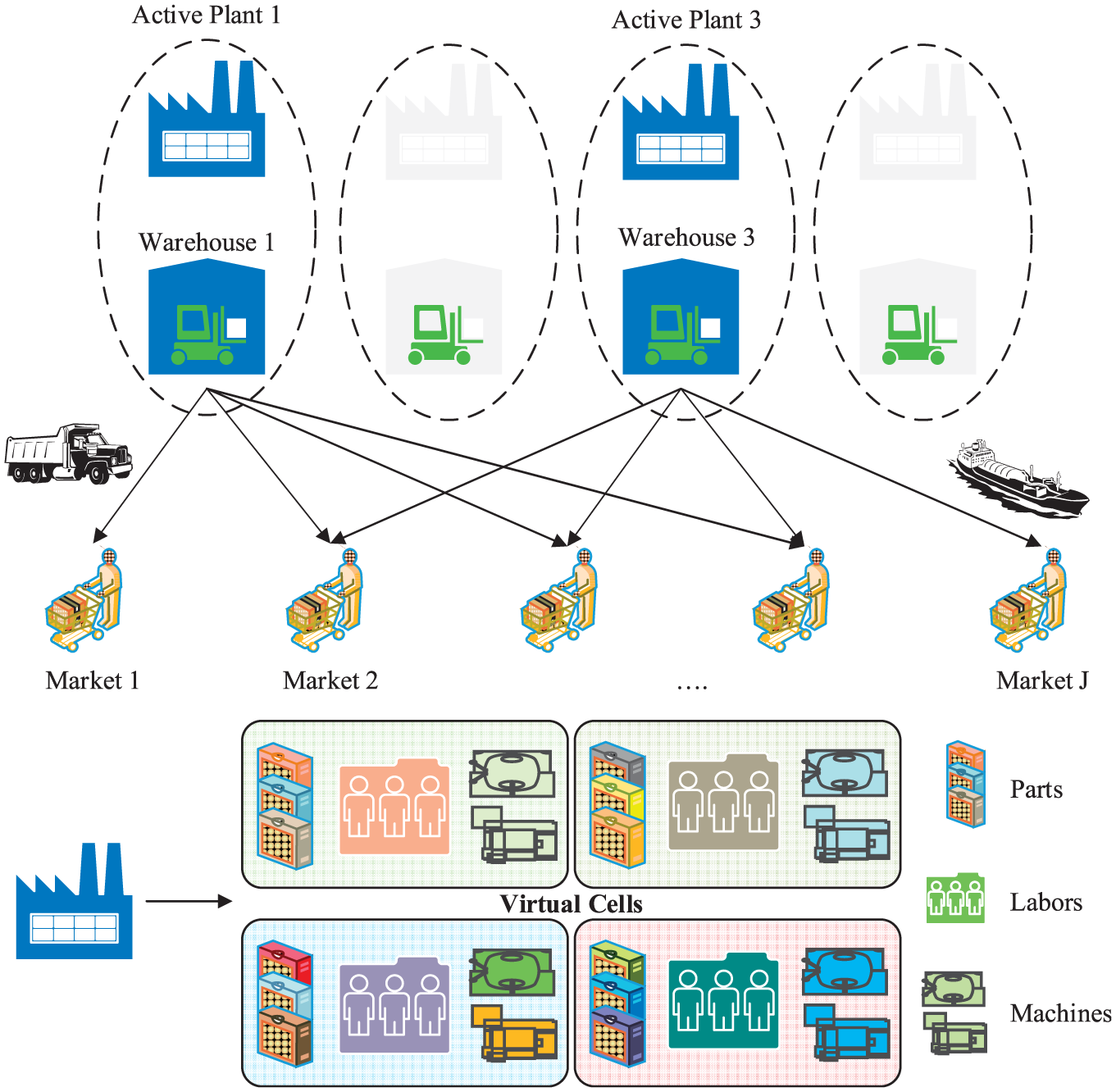
The structure of proposed model.
In the two-stage method, the decision-maker makes some decisions in the first stage. The second stage’s decisions are concluded through randomness events as well as the first stage’s decisions. A recourse decision could then be made in the second stage which compensates for any bad effect that might have been experienced as a result of the first-stage decision. The optimal policy of such a model is a single first-stage policy as well as a collection of recourse decisions (a decision rule) defining which second-stage action should be taken in response to each random outcome. Although the two-stage stochastic linear programs are often regarded as the classical stochastic programming modelling paradigm, the discipline of stochastic programming has grown and broadened to cover a wide range of models and solution approaches. The two-stage stochastic programming approach has various applications in different fields such as electric energy producers, 57 transportation network protection 58 and financial planning. 59 To the best of the authors’ knowledge, this is the first article in applying the two-stage stochastic programming to the DCMS.
The aim of the proposed model is to minimize the total cost of holding, inter-cell material handling, external transportation, fixed cost for producing each part in each plant, machine and salary labour. The main constraints are satisfaction of market demand, machine and labour capacity, production volume for each plant and the allocated amounts to each market. The first stage of the two-stage method identifies (1) the plant locations and (2) grouping parts–machines–workers’ assignment to virtual cells, which is fixed and independent of the scenarios, while the second stage determines (1) the production volume for each plant, (2) the allocated amounts to each market and (3) the operations’ allocation to the virtual cells. In this study, the following assumptions are considered:
Processing times of each part on each machine type are deterministic.
Market demand for each part type is uncertain.
The time capacity of each machine and labour type are known.
The number of virtual cells for each plant is given, and the lower and upper bounds of the cell size are also known.
Only single labour is allocated for processing each part on each corresponding machine type.
Inter-cell material handling cost is constant for all transfers regardless of distances. In other words, it is assumed that the distance between virtual cells is the same, the distance among machines at each virtual cell is the same and also all machine types have equal dimensions. Also, transferring the parts between manufactures is not allowed.
Holding inventories and outsourcing products are allowed between periods with identified cost, while backorder inventories are not allowed. In other words, all market demands must be satisfied.
Maintenance and overhead costs of each machine type are identified. These costs are measured for each machine in each virtual cell and manufacturer regardless of whether the machine is active or idle.
Salary cost of each labour type in each manufacture is known. This cost is considered for each labour in each virtual cell and manufacturer irrespective of whether the labour is active or idle.
Mathematical model

Subject to

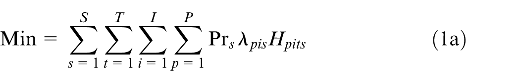
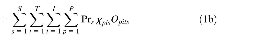
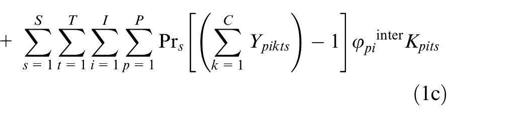
The objective function consists of eight cost terms as follows:
1a. Holding cost: the expected holding cost of inventory for all parts in the planning horizon in all scenarios.
1b. Outsourcing cost: this expected cost is related to the production outsourcing cost for active plants in the planning horizon in all scenarios.
1c. Inter-cell material handling: the expected cost of transferring parts between virtual cells, whenever parts cannot be produced completely by machines in a single virtual cell. The inter-cell material handling cost happens when parts are transferred between virtual cells. This occurs when parts need to be processed in multiple virtual cells, because all required machine types to process the parts are not available in the virtual cell in which the parts are allocated. This cost is calculated for the number of virtual cells greater than 1. In other words, when the parts can be produced completely in one virtual cell, then this cost is 0. Inter-cell moves reduce the efficiency of the CFPs by growing material handling requirements, flow time and complication of production control.
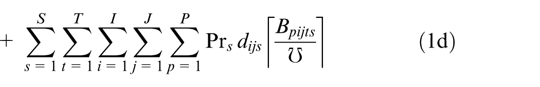
1d. Transportation cost: this term represents expected external transportation cost related to the distribution of finished products from each manufacturer to markets. In other words, this cost is related to the batch number of finished products to be transferred from manufacturer i to market j in the planning horizon in all scenarios.
1e. Fixed cost of production: this item includes the expected fixed production cost of each part type in each active plant in the planning horizon in all scenarios.
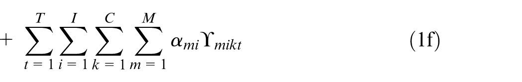
1f. Machine cost: this term refers to the maintenance and overhead costs of machines and is calculated based on the number of machines used in the virtual cell formation in the planning horizon.
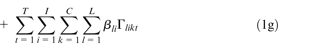
1g. Salary cost: the salary paid to workers in the planning horizon.
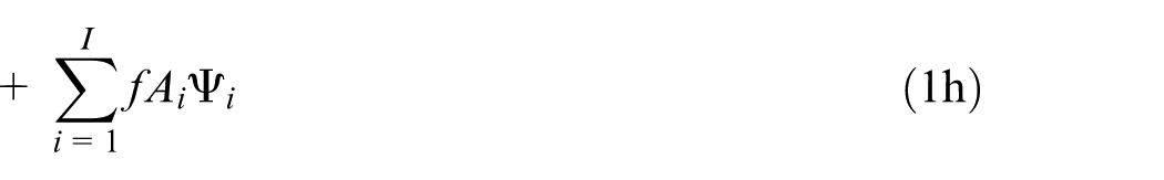
1h. Fixed cost of active plant: this term refers to the fixed production cost in active plants.
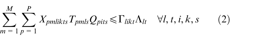
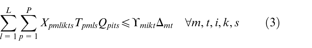
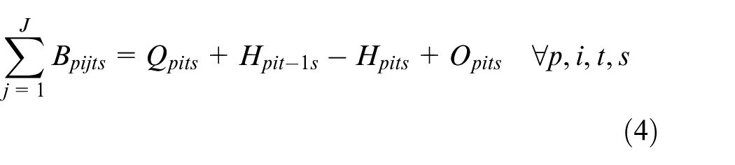
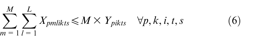
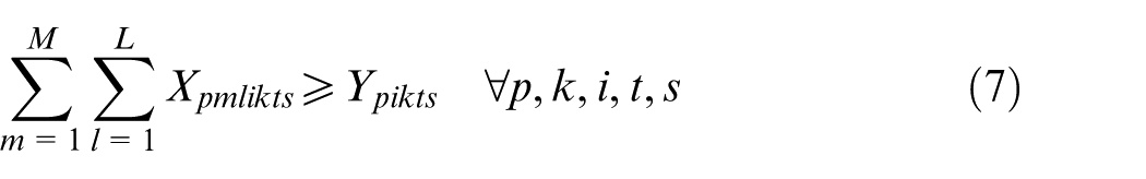
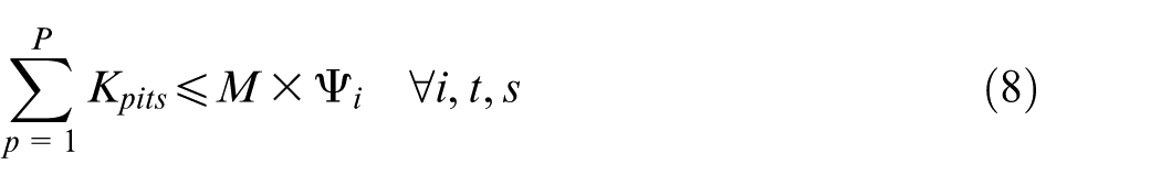
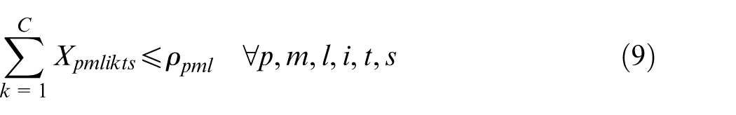
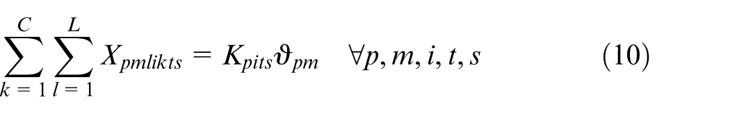
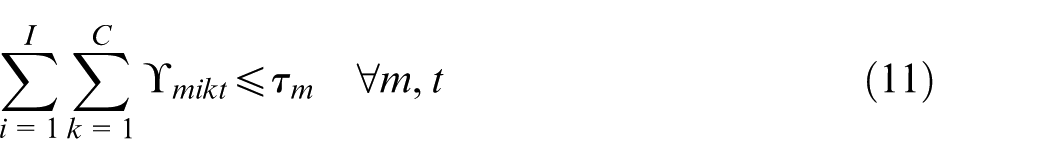
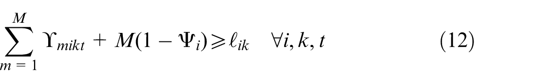
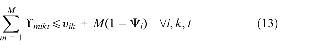
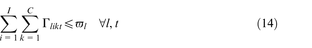
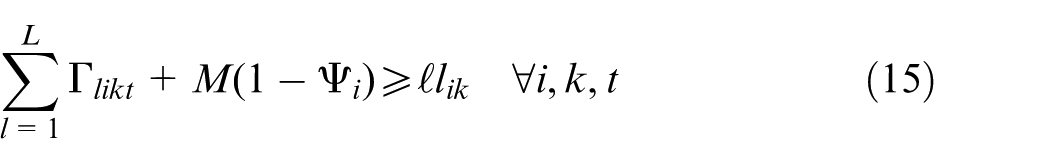
Constraints (2) and (3) enforce the time capacity of workers and machines to ensure they do not violate their boundaries. Equation (4) ensures that all market demands in the planning horizon must be satisfied. Constraint (5) implies that if part type p is produced in manufacturer i, then the production fixed cost of part p in this manufacturer is calculated. Constraints (6) and (7) determine whether part type p is processed within virtual cell k or not. Constraint (8) guarantees that each part type can be produced in manufacturer i if only this manufacturer is active. Constraints (9) and (10) imply that only one labour is allotted for processing each part on each related machine type. This model is flexible to enable a labour to work on several machines. This means that if one part is required to be processed on one machine type, more than one labour would be able to serve this machine type. Constraint (11) enforces that the entire number of machines of each type allocated to different virtual cells in all plants does not exceed the total number of available machines of that type. Constraints (12) and (13) specify the lower and upper bounds on the number of machines allocated to each virtual cell in all active plants. Constraint (14) guarantees that the total number of workers of each type allocated to different virtual cells will not exceed the total available number of workers of that type. Constraint (15) ensures that at least
Scenario generation
LHS
LHS was proposed based on Latin square experimental design, by McKay et al. 60 This method tries to eliminate confounding effect of several experimental factors without increasing the number of experiments. The aim of the method is to ensure that each value of a variable is represented in the samples, no matter which values can be more important. To illustrate this method, suppose that we have two independent random variables X and Y with uniform distribution and the goal is to generate five samples of these variables. According to the LHS method, the ranges of both X and Y are initially divided into five equal intervals, resulting in 25 cells as shown in Figure 2.
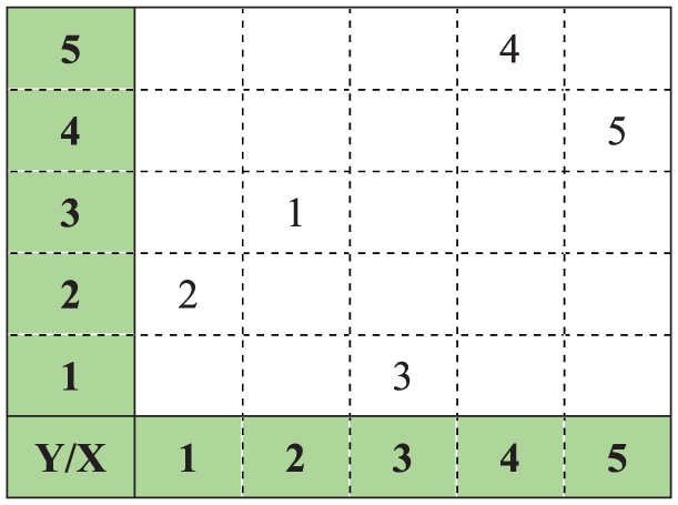
The Latin hypercube sampling method.
Of the requirements of this method is that each row and each column should include just one sample. This issue ensures that there are only five samples, and X, Y will be sampled from any of these five. For each sample [i, j], the sample values of X, Y are determined as follows

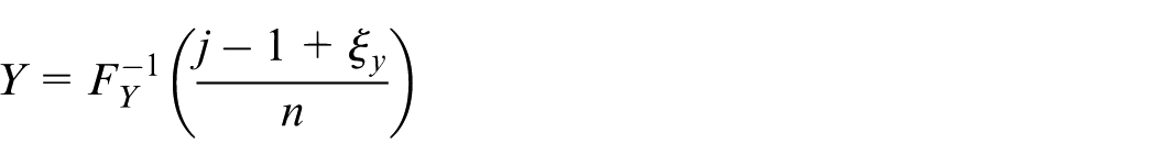
where n is the sample size,
SAA
Consider a stochastic programming problem in the form of
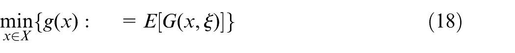
where
The SAA method is ideally suited for a parallel implementation. The statistical theory of the SAA estimators is closely related to the statistical inference of the maximum likelihood method and M-estimators. There are some well-developed statistical inferences of the SAA method. See a comprehensive review by Kleywegt et al. 62 The overall steps of SAA are as follows:
Sample sizes: choose initial sample size N for the first M sample and N′ for the second-phase sample of the algorithm.
For m = 1,…, M, solve the two-stage stochastic problem and provide objective value
Calculate the average of
By a feasible solution, for example, one of
Estimate the optimality gap as
If the optimality gap and the variance of the gap estimator are sufficiently small, go to Step 8.
If the optimality gap or the variance of the gap estimator is too large, increase the sample sizes N and/or N′ and return to Step 2.
Choose the best solution
GA for solving the two-stage stochastic problem
GA is a powerful meta-heuristic technique which implements the principle of natural selection. GA developed initially by Holland 63 searches the feasibility space and situation of feasibility solutions simultaneously in order to find the optimal or near-optimal solutions. The procedure is carried out using genetic operations. Goldberg 64 and Reeves65,66 gave an interesting survey of some practical works carried out in this area. The steps of the GA are presented as follows:
Step 1: Producing the initial solution of the two-stage stochastic problem. Create a random feasible parent or population P0 of population size; set t = 0.
Step 2: Evaluating fitness of the solution set. Assign a fitness value to each solution in P0 according to the objective function.
Step 3: Selecting mating pool members of the population size set by focusing on the fitness value. Tournament selection Roulette wheel selection Elitist selection with their rates to select the chromosomes from Pt
Step 4: Genetic operators Crossover Mutation Replacement
Step 5: If stopping criterion is satisfied, terminate the algorithm and return the best solution of the generation.
Step 6: Go back to Step 2 and set t = t + 1.
The flowchart of the GA algorithm process is shown in Figure 3. 67
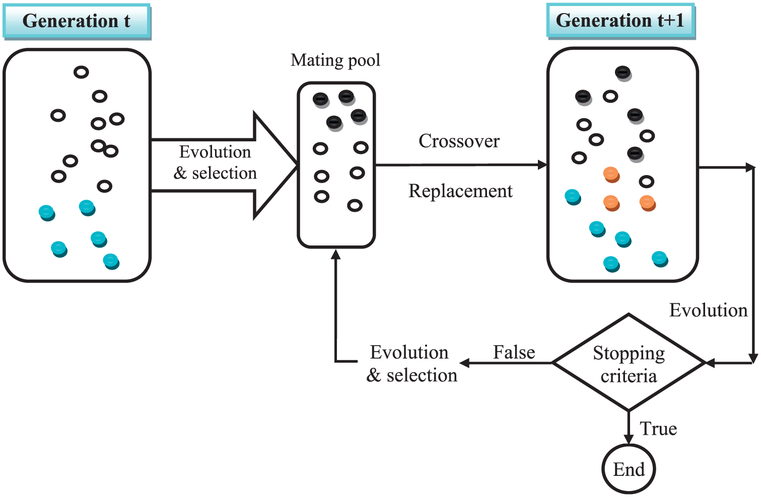
The flowchart of GA algorithm process.
The machine–part CFP is a NP-complete combinatorial optimization problem in CMSs. 68 Given this, it is obvious that considering dynamic situation in the proposed model, the complexity of the problem significantly increases, where solving such a problem using exact methods in real-sized cases is so hard/impossible in practice. So applying meta-heuristic algorithms is unavoidable for solving such a NP-complete problem.
Among the previous researches, GAs have been widely used to solve the machine–part CFP. Many researchers8,69–72 have revealed that the GA can yield high-quality solutions for CMS. In better words, by appropriate selection of GA’s parameters, selection strategy as well as crossover and mutation operators, one can obtain efficient and flexible solutions.
Solution coding (chromosome structure)
Solution structure representation is very important in each meta-heuristic approach and represents a feasible space solution of the problem. A solution structure consisting of five chromosomes is as follows:
1. The first chromosome is related to the location of each active plant, named matrix STR1. STR1 is (1 × I) genes with binary alleles as shown in Figure 4. For example, in Figure 4, it can be observed that plants 1, 4, 7 and 9 are active. Constraint (8) is naturally satisfied by this chromosome.
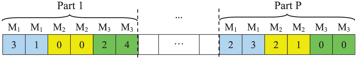
2. The second chromosome determines that each part of the operation is processed by which labour on which machine type. This chromosome is named matrix STR2 and is a four-dimensional matrix as shown in Figure 5. STR2 is S × T × I × (P × M × τ) with alleles of 0, 1, …, L. Alleles represent which labour does the process of a part on its corresponding machine. As can be seen in Figure 5, the problem consists of p part types and three machine types for which the number of available machines for each type is 2 and 4 labour types. For example, part type 1 is processed on the first and second machine type 1 by labours 3 and 1 in plant 1.
By completing the matrix STR2, constraints (6) and (7) are naturally satisfied by this chromosome, but constraints (9) and (10) might be broken during algorithm performance. So to keep these constraints remain feasible, the repair strategy is applied. In other words, the repair strategy transforms the infeasible solution to be feasible. In STR2 of the chromosome, the two corrections are as follows:
Alleles should take zero for situations where parts do not need machines.
In non-zero genes, the labour assigned to do the process should be capable of working with the related machine.
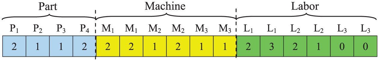
3. The third chromosome determines the part–machine–labour assignments. This chromosome is named matrix STR3 and is a three-dimensional matrix as shown in Figure 6. STR3 is T × I × (P + M × τ + L × ϖ) with alleles of 0, 1,…, C. Alleles identify the cell in which part, machine and labour are assigned. Constraints (11) and (14) are naturally satisfied by the chromosome, but constraints (12), (13) and (15) (the minimum and maximum sizes of cells) might be broken during the algorithm performance and the repair strategy is utilized.
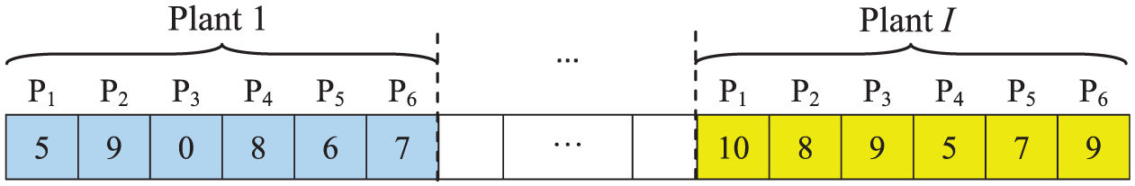
4.The fourth chromosome is related to the volume of each part in each plant under each scenario. This chromosome is named matrix STR4 and is a three-dimensional matrix (S × T × [I × P]) as shown in Figure 7. For example, in Figure 7, it can be observed that the number of product part type 2 in plant 1 is 9. By completing matrix STR4, constraints (2), (3) and (5) are naturally satisfied.
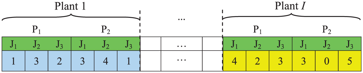
5. The fifth chromosome determines the number of finished products transferred from each plant to each market in each period under each scenario. This chromosome is named matrix STR5 and is a three-dimensional matrix (S × T × [I × P× J]) as shown in Figure 8. As can be seen in Figure 8, the numbers of finished products part type 1 transferred from plant 1 to markets 1, 2 and 3 are 1, 3 and 2, respectively. By completing this matrix, constraint (4) is naturally satisfied.
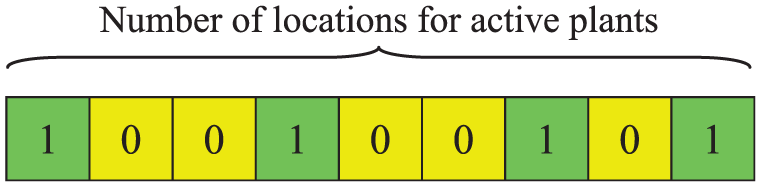
Active plants.
The process assignment of each part type.
Assignment of parts, machines and workers to cells.
The volume of each part type.
The volume of finished products transferred from each plant to each market.
Producing the initial solution
Determining proper population size in the GA is a major decision. If the selected number is too small, one may not be able to attain a good solution. Also, a large population size takes too much computational time so as to attain the final solution. This research has adopted a method to produce the initial solutions as follows.
Random method: Randomly chosen feasible parents produce the same number of initial solutions as the quantity of the solution set.
Evaluate fitness degree of solution set
The GA evaluates chromosomes based on a fitness function value. Namely, it focuses on the objective function and problem characteristics and transforms them into a mathematical function which is called fitness function. According to the objective function of the presented two-stage model, the chromosomes’ fitness must be obtained by calculating eight parameters

Selecting mating pool members
In order to create a new generation, it is required to select some chromosomes (mating pool) with the latest fitness in the generation progress for recombining or creating chromosomes allied to the new generation. In this context, Roulette wheel selection, tournament selection and elitist selection are used in which the fitness of the current generation of chromosomes is calculated according to the objective function.
Improved GA operators
To explore the feasible solution space, it is needed to generate other solutions which are made from the current ones. These new solutions are called neighbourhood. Subsequently, the feasibility of these solutions should also be investigated. If the obtained solution is infeasible, one should apply a repair strategy that transforms the infeasible solution to feasible one.
Crossover operator
Crossover operator is naturally utilized to swap some genes’ values from two chromosomes to create new individuals/offsprings. The used crossover method in this study adopts the common two-point crossover approach. Two tangent points initially made by the genes’ value of the two chromosomes are exchanging segments (between two tangent points) of the parent solutions, thus offspring solutions retain partial properties of the parent solutions. Since our problem has some constraints, the feasibility of the produced solutions/individuals is checked.
Figure 9 depicts two considered parents to make two offspring. To do so, two random cuts are made in the length of chromosomes. As it could be seen, these chromosomes are cut in genes numbers 4 and 10. Now, since we have two cut points, consequently the chromosome of each offspring has three parts. To fill the genes of each offspring, according to Figure 9, the first part of the first parent is assigned to the first offspring to fill the first part of it (in blue), the second part of the second parent is used to fill the second part of the first offspring (in yellow) and the third part of the first parent is used to fill the third part of the first offspring (in blue). The same scheme is utilized so as to constitute/fill the genes of the second offspring, according to Figure 9. In order to make the generated offspring feasible, a repairing process is utilized.
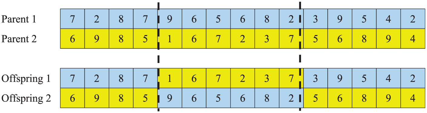
The schematic example of crossover procedure.
Mutation operator (intelligent mutation)
Mutation is a genetic operator employed so as to keep genetic diversity from one generation of a population of GA chromosomes to the next. The mutation operator chooses randomly ones among the genes of all parents in the population with a fixed mutation rate. This probability should be set low. If it is set too large, the search will turn into a primitive random search. This operator can be applied by inverting part of a gene in a parent chromosome to obtain the offspring chromosome.
As it could be observed from Figure 10, the two numbers are randomly selected to swap their values with each other. In this schematic example, numbers 5 and 10 of the parents are selected. Then, the values of these genes are exchanged with each other to constitute new offsprings.
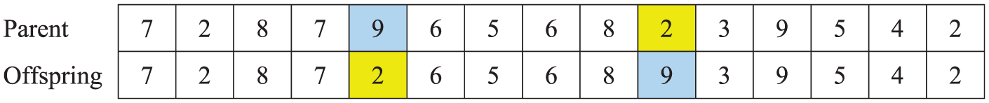
The schematic example of mutation procedure.
Termination of GA
The GA continues to create a population of offspring solutions until a criterion for stopping is met. In this algorithm, the stopping criterion is the maximum number of generation, that is, the algorithm ends functioning when a specified number of the generation is reached.
Experiment data analysis
Taguchi experimental design
The application of Taguchi method has attracted more attention in the literature for the past 20 years, and nowadays Taguchi method has been widely applied to various fields, such as manufacturing system 73 and mechanical component design. 74 The popularity of Taguchi method is owing to its practicality in designing high quality systems that provide much reduced variance for experiments with an optimum setting of process control parameters. Taguchi method, based on fractional factorial experiments (FFEs), is an influential instrument to optimize product and performance of the processes. Taguchi splits the factors into two main categories: controllable and noise factors. Noise factors cannot be directly controlled. Since removal of the noise factors is unreasonable and often impossible, Taguchi method seeks to minimize the effect of noise and determine the optimal level of the important controllable factors based on the concept of robustness. 75 In addition to determining the optimal levels, Taguchi method establishes the relative importance of single factors in terms of their main effects on the objective function. Taguchi method formed a transformation of the repetition data to another value which is the measure of variation. Taguchi method is a robust design approach developed by Taguchi et al. 76 which uses many ideas from statistical experimental designs for evaluating and implementing improvements in industries. Actually, Taguchi method is an instrument to conduct experiments through a statistical approach to understand the significance of independent factors and levels. Taguchi method is a robust experimental design that seeks to obtain a best combination set of factors/levels with lowest cost solution to achieve product quality requirements. It also comprises several functional elements which can provide the necessary contribution needed to improve the optimization implementation. After further analysis, the best parameter level combinations could be tuned. When conducting production using this set of parameter levels, the representative of the quality characteristic will be mostly close to the objective function and has the smallest variances. The two main tools employed by Taguchi method are the orthogonal array and the signal–noise (S/N) ratio. The S/N ratio measures quality, while orthogonal arrays are used to study many design parameters, simultaneously.
The main advantage of Taguchi method is that the number of experiments conducted in most of the cases is lesser than that of any other experiment using a statistical approach. Taguchi method is utilized in this article, since it is known as a cost-effective and labour-saving technique. It can also investigate four factors simultaneously that will affect the solution quality and assign the level number as three levels to accomplish the parameter design. Moreover, it proposes the level range design based on a real experience as well as the results of discussed literature.
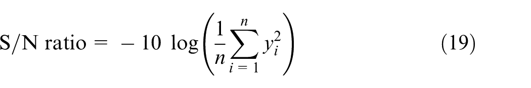
The S/N ratio indicates the amount of variation which exists in the response variable. The objective is to maximize S/N ratio. There are several categories of S/N ratio, depending on the type of characteristic: lower is better, nominal is the best and higher is better. 77 Since almost all objective functions in scheduling are classified in the ‘lower is better’ type, their corresponding S/N ratio is calculated according to equation (19) as follows
Parameter design in the GA
The impact of fine-tuning of operators and parameters on the performance of the algorithm is comprehensively investigated by means of Taguchi method as an optimization technique. Taguchi method is utilized in this article, since it is known as a cost-effective and labour-saving technique. It can also investigate four factors simultaneously that will affect the solution quality and assign the level number as three levels to accomplish the parameter design. Moreover, it proposes the level range design based on a real experience as well as the results of discussed literature. Thus, L9 inner orthogonal array supported with L5 outer orthogonal array is adopted to satisfy all requirements. Hence, GA parameters and their level values are illustrated in Table 1.
GA parameters and their level values.
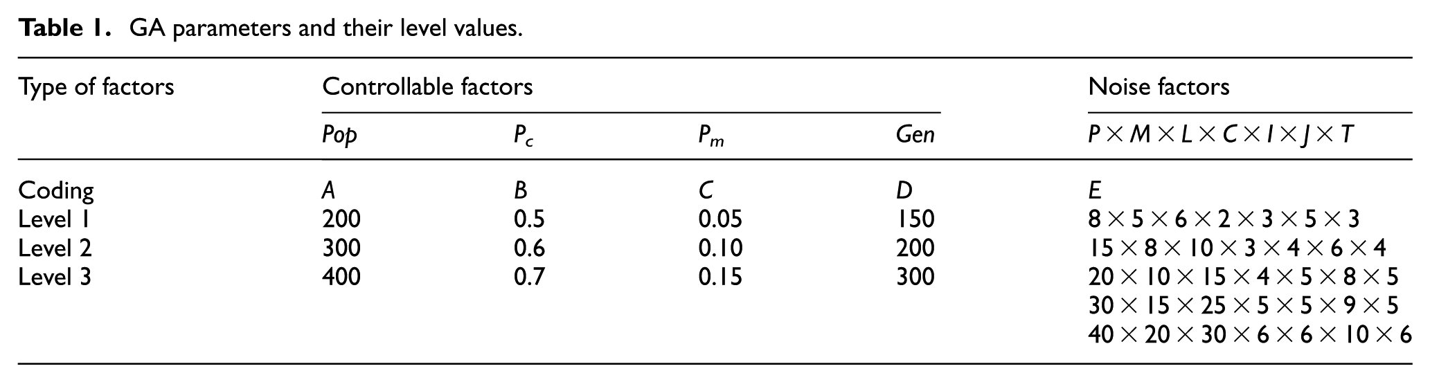
The factors that should be tuned are probability of crossover (Pc), probability of mutation (Pm), population size (Pop) and the number of generation (Gen). Three levels are considered for each factor in the experiments. For the cases of crossover, the performance of the above-mentioned operators is tested. The levels of Pop are considered as 200, 300 and 400, while the levels of Pc are regarded as 0.5, 0.6 and 0.7. Also, the levels of Pm and Gen are considered as 0.05, 0.1, 0.15 and 150, 200 and 300, respectively. We run GAs for each of the Taguchi experiment, and then the obtained data are transformed into S/N value. Finally, the obtained graph is illustrated in Figure 11.
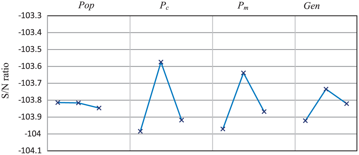
The mean S/N ratio plot for each level of the factors.
The optimal levels of factors A, B, C and D are A(1), B(2), C(2) and D(2), respectively. The analysis of variance (ANOVA) is also carried out to obtain the relative importance of each single factor in terms of their main effects on the response variable which is shown in Table 2. It is necessary to indicate that the freedom degree of error is zero, and consequently, the conduction of ANOVA is impossible. We therefore consider factor crossover type as ‘error’ to consider its freedom degree as error one. We have selected the crossover type, since it has the ‘least mean square’ which means that it definitely has the least relative importance. According to the obtained results summarized in Table 2, Pc has the greatest effect on the algorithm’s quality with a relative importance of 55.67% while the second high impact factor is Pm with almost a relative importance of 33.05%. The relative importance of Gen is 9.77%.
ANOVA table for S/N ratio.
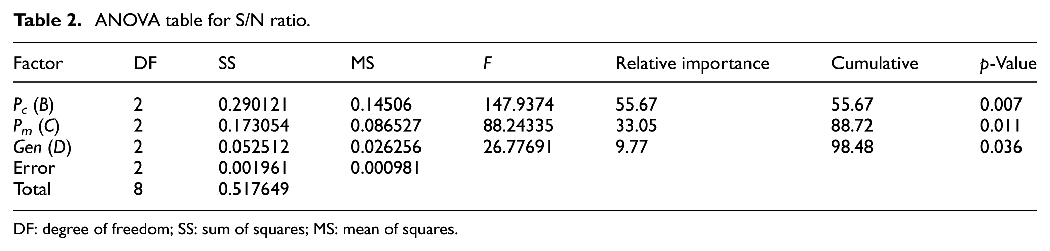
DF: degree of freedom; SS: sum of squares; MS: mean of squares.
Computational results
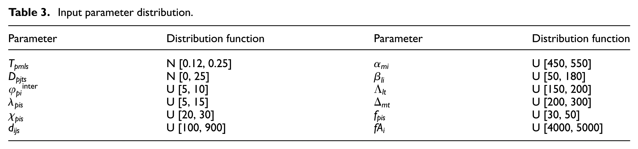
All calculations are carried out using the CPLEX 9.0 solver engine of the GAMS software and are accomplished on a PC with core i5 CPU and 4 GB of RAM. It has been chosen to solve all cases using M = 3 SAA problems. This model is very complex and consists of a large number of variables. So we have to select a small size of scenario set, since by increasing the scenario number, solving computational time also grows rapidly. To avoid spending a long time for solving the model, sample sizes N = 5, 10, 15 and 20 scenarios are employed for instances with 20 parts, 10 machines, 15 workers, 4 cells, 5 plants, 8 markets and 5 periods. The other parameters such as demand and processing times are generated over a normal distribution with proper specifications. Table 3 shows the distribution function of each input parameter.
Input parameter distribution.
For the disaggregated problem instance, we normally get an optimality gap less than 1% as the termination criteria. The result of the SAA method is shown in Table 4.
Results of SAA.
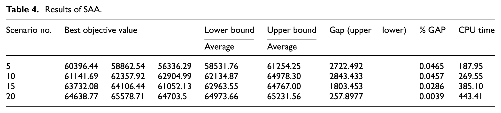
In Table 4, the best solution obtained by solving the SAA problem has been presented with the different sample sizes. The estimator for the optimality gap is calculated by subtracting the lower bound from the upper bound. As it could be seen in Table 4, in scenario #20, the optimal gap is obtained and the algorithm could then be terminated. This matter occurs, since the average SAA value for the lower bound (64973.66) is the largest one for scenario #20 with respect to the others. On the other hand, scenario #20 has the lowest variation value among the existing scenarios which leads to the lowest optimality gap among the other alternatives. It should also be pointed out that the execution time of this scenario is considerably larger than the others. This issue could be interpreted as the computational complexity of the algorithm.
The confidence interval for the optimality gap is getting narrower as the number of scenarios in the SAA problem increases. This is mainly due to smaller variance of the lower bound. So by increasing the number of scenarios, converging to optimal solution is more likely.
As it could be implied, the computational time increases whenever the number of scenarios grows. For example, in the case of five scenarios, the CPU time is 187.95 s, while by increasing the scenario number to 20, the computational time increases to 443.41 s. Figure 12 demonstrates the convergence diagram of the employed GA in the SAA technique for 20 scenarios.
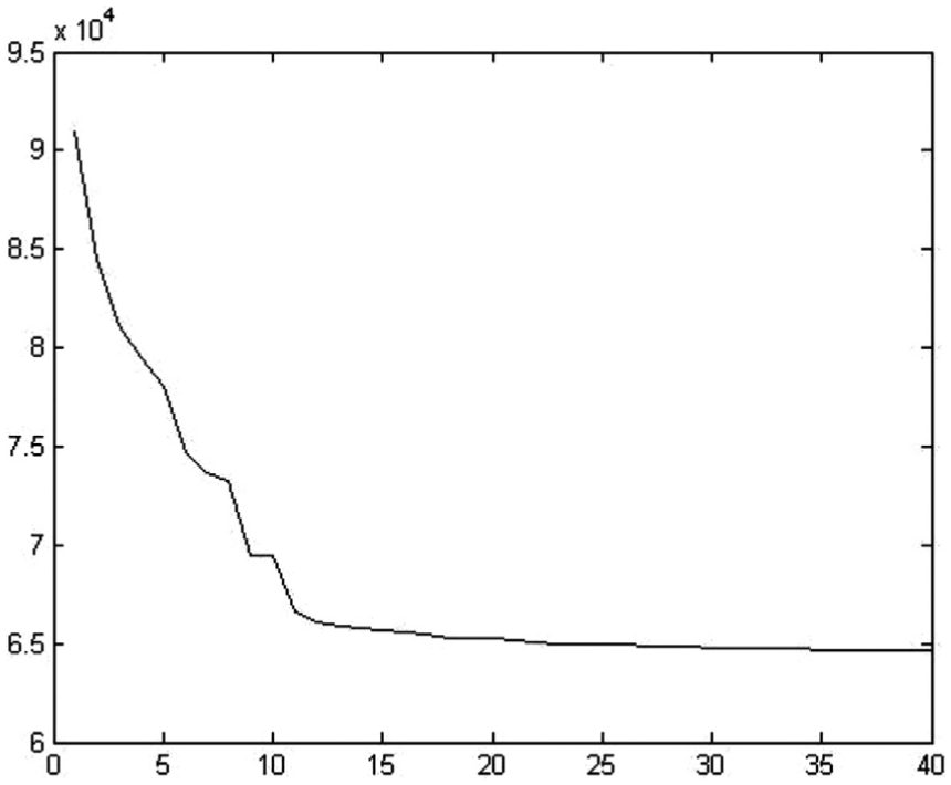
The algorithm convergence with 20 scenarios.
The algorithm converges to the best solution after about 40 iterations. Accordingly, one could decrease the iteration number which leads to a reduction in spending computational time.
Value of stochastic solution
In this section, it should initially be shown that considering stochastic parameters such as processing time and product demand plays a vital role in the objective function. To do so, the problem has been solved in three different sizes (as represented in Table 1), each of which has been run five times. The computational results are demonstrated in Table 5 in which the following values are computed according to Birge and Louveaux: 78 here-and-now-solution (HN), wait-and-see-solution (WS), expected value of perfect information (EVPI), expected value of deterministic solution (EVS) and value of stochastic solution (VSS).
Main computational results on two-stage model.
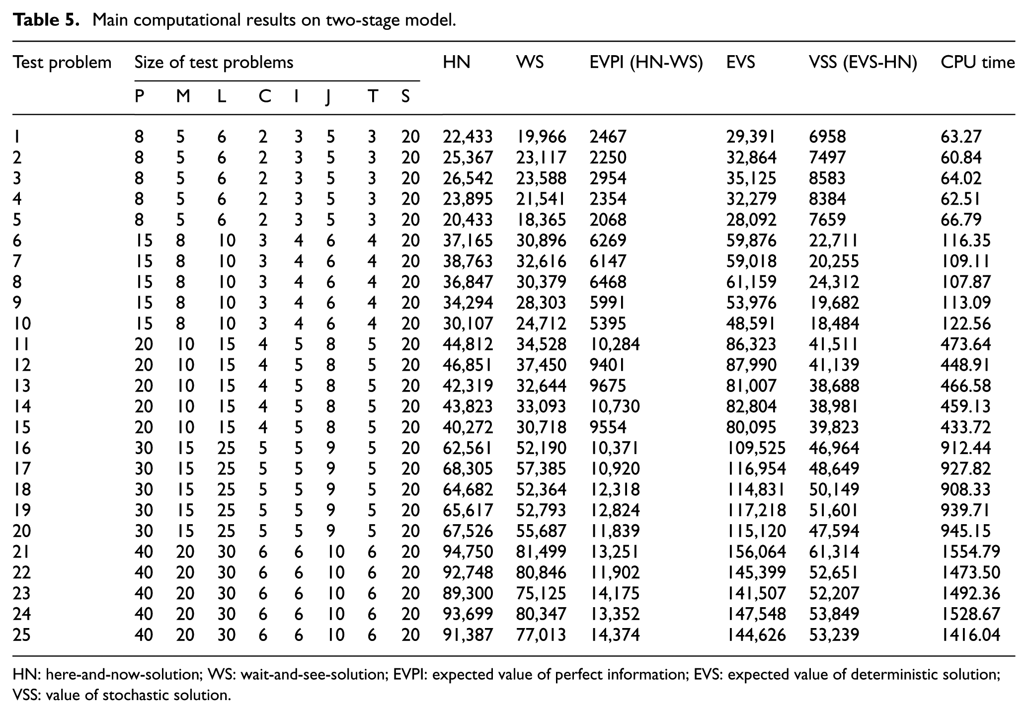
HN: here-and-now-solution; WS: wait-and-see-solution; EVPI: expected value of perfect information; EVS: expected value of deterministic solution; VSS: value of stochastic solution.
EVPI, in fact, is the loss caused by the existing uncertainty or the expected profit value when having perfect information. VSS assesses the value of knowing and using distributions on future outcomes. In other words, VSS represents the potential profit from solving the stochastic model and problems with no further information about the future. Accordingly, one can imply that VSS is more practical in reality.
According to Table 5, the EVPI could be calculated as the weighted objective function of all test problems. For example, in test problem #1, EVPI equals to 2467, and to calculate the VSS we replace the demand and processing time by their mean value and solve the model to obtain the expected value. Also by substituting the value of the obtained variable from expected value in the stochastic model, the quantity of EVS could then be computed. In test problem #1, this value equals to 29,391. Since VSS is the difference between EVS and HN, for the above-mentioned instance, the value of VSS will be 6958.
As it could be observed in Table 5, the computed EVPI values in all test problems are less than their corresponding VSS values. It means that solving the stochastic model is more beneficial compared to the situations where more information is available through more extensive forecasting, sampling or exploration. Consequently, it is valuable to consider stochastic parameters for the proposed model.
According to Table 5, whenever problem dimensions increase, the values of EVPI and VSS also increase. The true interpretation for such phenomena is that the value of information in large-scale problems is high and uncertain parameters will be more effectual. In Figure 13, the average VSS values for different sizes are depicted. It could be observed that the VSS gradient for small and medium sized problems is much sharper in contrast to large-scale problems when the problem size gets larger. This could be interpreted as a lower growing gradient for stochastic parameters of the model in a large-scale problem.
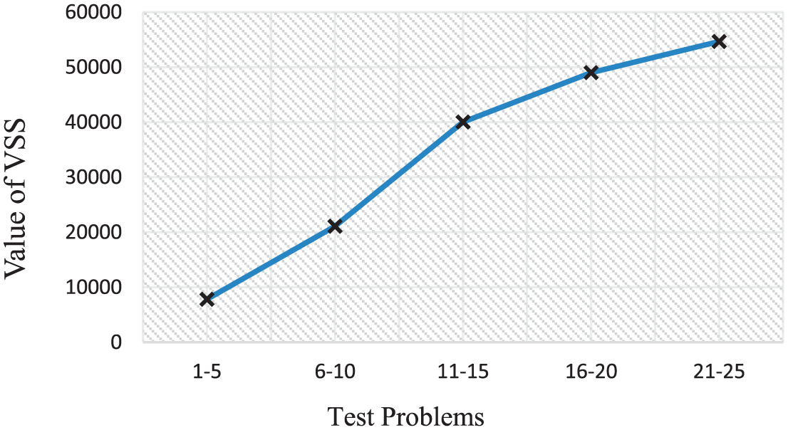
Average of VSS for each size.
Another issue which should be pointed out according to Table 5 is that the solution time of the two-stage model by GA increases exponentially when the problem size gets larger. This matter implies that the execution time of the algorithm grows considerably by increasing the problem size. In Figure 14, the average CPU time for each size is depicted.
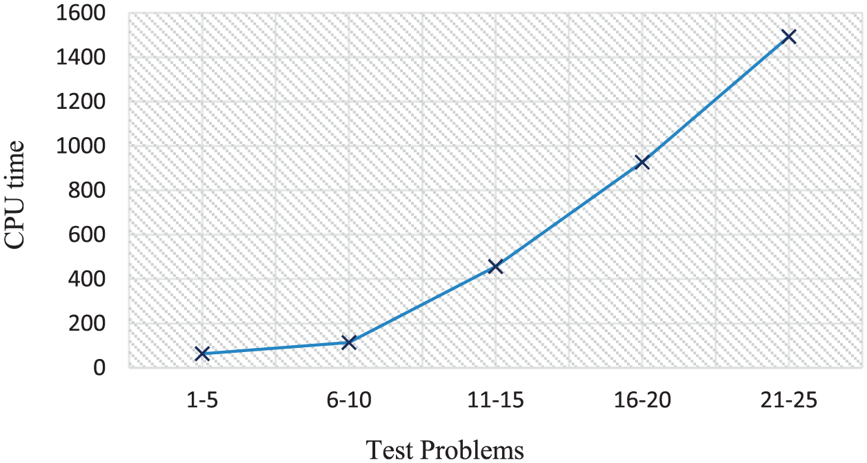
Average of CPU time for each size.
Conclusion and further research
In this article, we introduced a two-stage approach to solve a DVCMS in multi-plant location, multi-market allocation and production planning. The presented model considering stochastic parts’ processing time as well as the products’ demands are described by discrete scenarios. The first stage of this method determines the plant locations and grouping parts–machines–workers’ assignment to cells, while the second stage identifies the production volume for each plant, the allocated amounts to each market and the operations’ allocation to the cells. The goal of this model is to minimize the total cost of holding, inter-cell material handling, external transportation, fixed cost for producing each part in each plant machine and salary labour.
Due to the complexity of the proposed stochastic problem, a GA was developed to solve it in a reasonable computational time. Four factors that affect the solutions’ quality, that is, population size (Pop) probability of crossover (Pc), probability of mutation (Pm) and number of generation (Gen), were tuned by means of Taguchi method to determine the optimal level of these factors. Also, ANOVA was carried out over the results to obtain the relative importance of each single factor in terms of their main effects on the response variable.
The contributions of this research are as follows: (1) considering stochastic parameters leading to more flexibility and practical aspects in real-world cases, (2) presenting a two-stage approach for solving the DVCMS in multi-plant location, multi-market allocation and production planning, (3) developing a GA which had successful performance in any size of the problems and (4) generating discrete scenarios with LHS and SAA.
As a direction for future research, it would be interesting to investigate the following directions:
Development of the model under other stochastic parameters such as costs, machine failure, machine and labour availability. 21
Applying the multi-objective approach to solve the considered problem in which the CFP decisions could be optimized in one objective while production planning is optimized in the other.
Aggregating other production aspects like layout problem considerations and scheduling into the proposed model.79,80
Working on other solution methods such as other stochastic algorithms as well as other newborn meta-heuristic techniques such as intelligent water drops (IWD) algorithm as a powerful technique in this area so as to achieve even better results.81–84
Footnotes
Appendix 1
Appendix 2
In this section, in order to verify the presented mathematical model, a small example is solved including complete input data and complete results. In this example, there are five markets where their demands in pessimistic (the lower value of demands) and optimistic (the higher value of demands) scenarios are considered with equal probability, that is, 0.5.
In this example, it is assumed that we have two alternatives for establishing facilities, each of which includes three virtual cells. Now we are looking for a suitable location of factories so as to meet all market demands. It should be pointed out that the fixed costs of establishing factories in locations 1 and 2 are 7.8 and 8 million dollars, respectively.
This example includes five machine types, eight part types and four labour types. All data are given in Tables 6–9 which correspond to the machine, part, labour and plant and market information. Moreover, the number of virtual cells to be formed is fixed at 3, and the minimum and maximum cell sizes for the number of machines in each cell in each plant are 1 and 3, respectively. The minimum size of each cell in each plant in terms of the number of labours is assumed to be 1. In this example, the available number of each machine and labour type is 2. The costs of related machines and labours are presented in Tables 6 and 7, respectively. In Table 8, machine types 1, 2 and 4 are required for part type 2. Moreover, the demand quantity for each period as well as set-up, material handling costs, holding and outsourcing costs and fixed cost of productions are presented in Table 8. As it can be seen in Table 9, the distance from plants to each market and also the number of products in each batch are 10. The data set related to the processing time matrixes and the other data of the case study are presented in Table 10.
The obtained optimal solution and the results of this example are presented in Tables 11–13. The production volume for each plant and the amounts allocated to each market in each period as well as the objective function value are shown in Tables 11 and 12, respectively.
As it could be observed from Table 12, the outsourcing and holding costs of products are 0, since all requested products by markets in each period and each scenario are produced by factory 2 in that period and then sent. Also, as it could be implied, the expected (average) value of total costs is about 30 million dollars.
These results indicate that among two alternatives for the construction of manufacturers, only one plant in location 2 will be activated. Furthermore, no products will be produced in factory 1.
Table 13 indicates the parts’ assignment, labours and machines to different cells in each plant and period. Moreover, it shows that labours 1 and 2 are assigned to cell 2 while labours 3 and 4 are assigned to cell 1 within period 1 in plant 1.
Declaration of conflicting interests
The author(s) declared no potential conflicts of interest with respect to the research, authorship and/or publication of this article.
Funding
The author(s) received no financial support for the research, authorship and/or publication of this article.