
Abstract
The hazard rate curve of the numerical control machine tool is a bathtub curve. The change point between the early failure period and the random failure period of the curve is difficult to obtain with a small data sample; thus, a Bayesian method is proposed. A method to build the prior distributions of the Weibull parameters is developed, which integrates the multi-source prior information of the target numerical control machine tool and the reference numerical control machine tool. The Markov chain Monte Carlo method is adopted to calculate the estimators of the Weibull parameters corresponding to each failure, which solves the problem of the absence of an analytical solution. The total working time of the numerical control machine tool when the estimator of the shape parameter is equal to 1 is estimated by taking the estimator of the shape parameter as the function of time. As a result, the change point and the early failure period are obtained. Comparison result shows that the result obtained through an existing change point solving method with a large dataset is close to the result generated through the proposed method with a small dataset. The change point and the early failure period obtained with the proposed method can be used to guide the early failure test and to design a rational maintenance strategy, which are of vital engineering significance.
Keywords
Introduction
Numerical control machine tool (NCMT) is a complex mechanical–electrical–hydraulic system, and its hazard rate (HR) function presents a bathtub curve as the working time changes.1–3 According to the failure frequency, the life cycle of the NCMT is divided into three stages, namely, the early failure period, the random failure period, and the wear-out failure period. The early failure period is caused by the defects in the design, poor processing precision of consistency, welding flaws, cracks, and poor assembly process consistency control,3–10 and the HR in this period is high and rapidly decreases as the working time increases. After reaching the random failure period, causing by random loads, human error, environment,3,5,7,8 and the HR is approximately constant.11–17 The time point when NCMT enters into the random failure period from the early failure period is defined as the change point of the bathtub curve. The change point is a significant reference for manufacturing enterprises to expose the potential failures of NCMTs by conducting an early failure test. Ideally, the NCMTs have totally entered the random failure period before the NCMTs are shipped to users or put into field operation. 3 Based on the change point, the manufacturing enterprises can establish rational maintenance strategies for different failure periods, which is significance to productivity improvement and maintenance cost reduction.17–19
Several studies have solved the change point of the bathtub curve. For example, Clarotti et al. 11 used a piecewise model to approximate the bathtub curve and to find the change point. Ülkü and Yenigün 12 used a piecewise constant hazard function with a change point; two estimation methods based on the maximum likelihood ideas are considered. Nguyen 13 considered the HR function as a two-section piecewise function to determine the change point. Gupta et al. 14 utilized the extended Weibull distribution to estimate the change point of the Bathtub curve by the maximum likelihood. Bebbington et al. 15 and Kim 16 defined the change point of the bathtub curve as the point where the curvature of HR curve has the maximum value. Jiang 17 proposed a non-parametric approach to estimate the empirical HR function and a cluster analysis method to find the change point. Bebbington et al. 20 used the empirical estimation method to obtain the change point of the HR function of the modified Weibull distribution. Pham and Nguyen 21 used a non-regular model and the bootstrapping method to find the change point. Jiang 22 proposed to use spline functions to approximate the degradation process and to find the change point.
The above methods are all based on large data samples. However, NCMTs have recently presented an obvious trend in production as shown by small lot and customization, rapid model upgrading, and improving reliability level. All these features result in the inadequate failure data of NCMTs in a reliability test and in the difficulty in obtaining the large data sample required by the classical statistic methods in a limited test time. Therefore, the existing methods are unsuitable for finding the change point of the bathtub curve with a small data sample. Thus, a Bayesian method that utilizes prior data to estimate the change point of the HR curve for NCMT is proposed. This method comprises four steps: (1) establishing a Bayesian model for solving the change point, (2) solving the prior distributions of the parameters of the reliability model, (3) calculating the posterior distributions of the parameters and the parameter estimators, and (4) solving the change point.
Bayesian model
Building the prior distributions of Weibull parameters
Weibull distribution and its function
According to the previous research experience on the reliability of NCMT, the two-parameter Weibull distribution is selected as the reliability model of NCMT.22–27 TBF r (time between failures, r = 1, 2, …, n), the time between the rth and r+ 1th failure, is a random variable. TBF r is independent and comes from the same population TBF, which follows a two-parameter Weibull distribution. The cumulative distribution function (CDF) and the probability density function (PDF) are expressed as follows
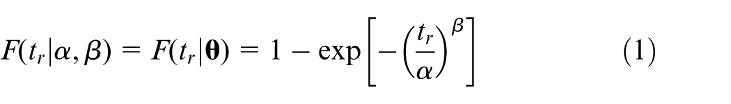
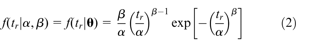
where tr is the observed value of TBF r , α> 0 is the scale parameter, β> 0 is the shape parameter, and θ = (α, β) is the parameter vector.
This section aims to establish the prior distributions of α and β. However, α and β do not have obvious physical meanings and cannot be understood directly by experts; 28 thus, some other quantities that can be easily judged by experts should be given.
MTBF (mean time between failures) and STD2 (square of standard deviation) represent the expectation and variance of TBF, respectively, which can be obtained by the following formulas
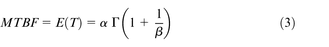
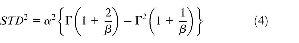
The unit of MTBF and STD is hours. Gutiérrez-Pulido et al. 29 considered that describing TBF with mean value and standard deviation (SD) is easy. Therefore, MTBF and STD are selected as the quantities whose value ranges can be given by experts.
Expert judgment procedure
The expert judgment procedure includes four stages, and each stage includes one or more steps:
Stage 1 is the preparation stage, which includes four steps:
Step 1.1 selects the reference NCMT according to the target NCMT (NCMT to be tested). The type, model, structure, and function of the reference NCMT should be similar to the target NCMT. The reference NCMT should have a large sample of field reliability test data. The best situation is where the target NCMT is upgraded based on the reference NCMT.
Step 1.2 collects the related information of the reference and target NCMT.
Step 1.3 selects the reliability model (two-parameter Weibull distribution) and model parameters (α and β) and determines the judgment quantities (MTBF and STD).
Step 1.4 defines the meaning of MTBF and STD and determines the multi-source of prior information.
Stage 2 includes two steps, in which the technique experts learn and practice their scoring skill:
Step 2.1 invites the technique experts to learn and practice their scoring skills repeatedly to reduce the subjective bias. The technique experts are the representatives of experienced NCMT designers, manufacturing staffs, outsourcing staffs, after-sales service staffs, NCMT operators, and NCMT maintenance staffs.
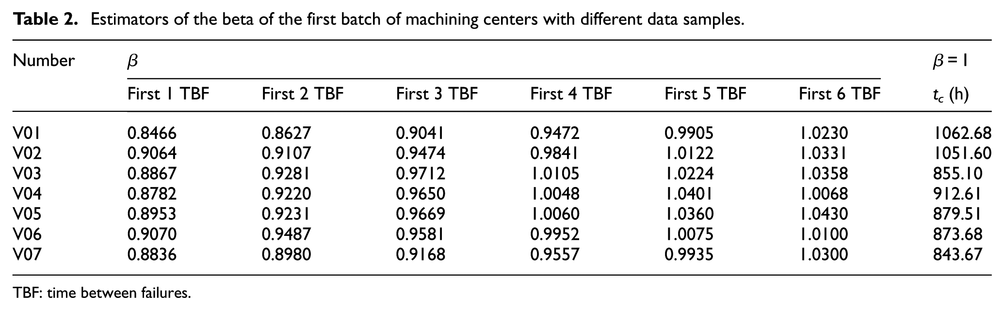
Step 2.2 asks the technique experts to master the multi-source prior information on the reference and target NCMTs. The multi-source prior information includes the following:
1. Basic information of NCMT (type, model, manufactory, manufacture date, and price).
2. Comparative analysis of the reliability levels of the sub-systems or components between the reference and target NCMTs.
3. Information on the reliability test of the reference NCMT and the value ranges of its MTBF and STD.
4. Operation behavior of the target NCMT in the reliability test, which includes stability, failure occurrence, failure cause, and failure mode.
Stage 3 asks the technique experts to score and obtain the judgment result. In this stage, the technique experts formally provide the value ranges of MTBF and STD for the target NCMT based on the practice in Stage 2 in combination with the multi-source prior information.
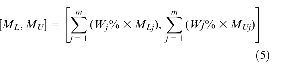
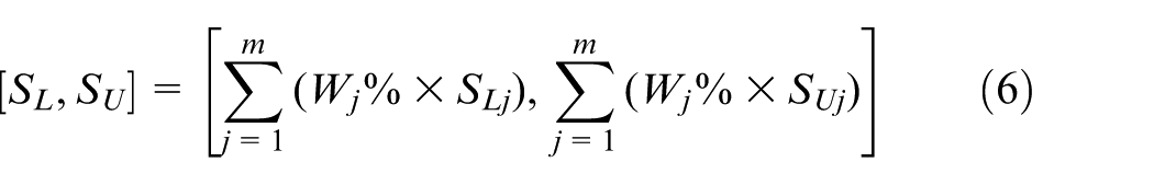
We assume that the number of the expert is m, and the value ranges of MTBF and STD given by the jth (j = 1, 2, …, m) expert are [MLj, MUj] and [SLj, USj]. A weight Wj% is first assigned to the jth expert to indicate his importance or his judgment accuracy based on his experience and degree of familiarity with judgment skill to integrate the judgment results of all experts into two single intervals, [ML, MU] and [SL, US]. The sum of all Wj% should be equal to 1. Thus, the final judgment is given as follows
Stage 4 is the feedback stage of the reliability test of the target NCMT. According to the reliability test status, testers determine whether the test should be continued. If the test should be continued, testers feed the failure and maintenance data in the test back to the experts; if the test should be ended, the prior distributions should be obtained, and the final report should be made.
MTBF and STD
MTBF is a direct indicator of the reliability of NCMT. If experts assert that NCMT A is more reliable than NCMT B, then the MTBF of A should be higher than the MTBF of B. STD is the indicator of the difference between tr and MTBF, as well as the indicator of stability or uncertainty of the NCMT. For two products A and B, experts can compare the reliability levels and the degree of difference between tr and MTBF based on experience and prior information.
From the point of HR, when β<1, NCMT is in the early failure period; when β = 1, NCMT is in the random failure period; when β> 1, NCMT is in the wear-out failure period. 9 The ratio between MTBF and STD depends only on β, which is demonstrated by the following formula
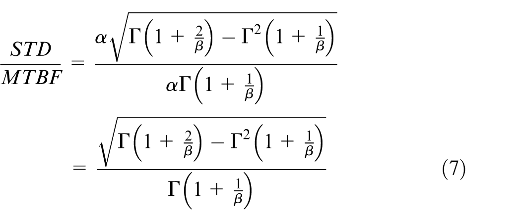
In (0, ∞), STD/MTBF is a monotonically decreasing function of β and approximates to 0 infinitely as β increases. Therefore, when STD/MTBF> 1, NCMT is in the early failure period; when STD/MTBF=1, NCMT is in the random failure period; when STD/MTBF<1, NCMT is in the wear-out failure period.
Transforming expert judgment into prior distributions
Building the prior distributions of Weibull parameters consists of three steps. First, a pair of point estimators of MTBF and STD is transformed into a pair of point values of α and β. Second, the estimation intervals of MTBF and STD are transformed into the intervals of α and β. Third, the prior distributions of α and β are built based on their intervals.
Transformation of point values
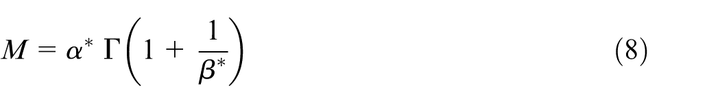
M and S are assumed as the two point estimators of MTBF and STD and (M, S) can be transformed to a pair of point estimators (α*, β*). From equations (3) and (4), (α*, β*) should meet the following two equations
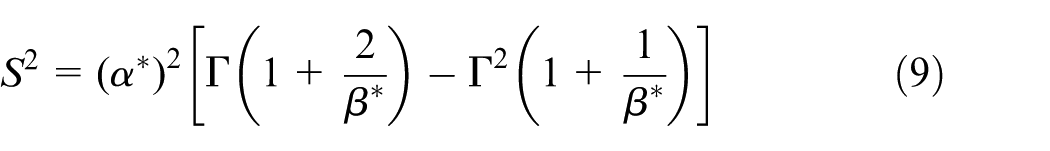
α is removed from equations (8) and (9)
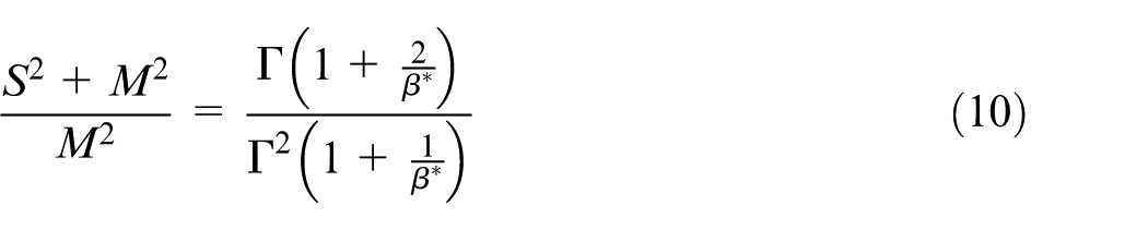
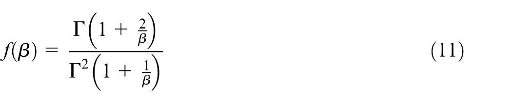
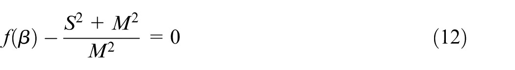
To obtain β*, we define the following function of β
The solution of the following equation will be the value of β*
According to the property of the gamma function,
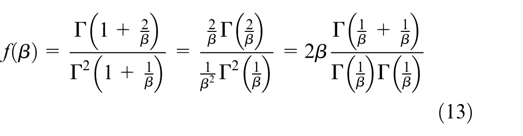
According to the relation between the beta function and gamma functions
We can have
According to equation (15), the curve of f(β) is plotted; f(β) is a monotonically decreasing function of β in (0, ∞) and approximates to 0 infinitely as β increases. Therefore, the abscissa of the intersection point of the curve of f(β) and the horizon line y = [(S2 + M2)/M2] is the value of β*. The solution of β* can be obtained with a numerical method. α* can be determined by equation (8).
Transformation of intervals
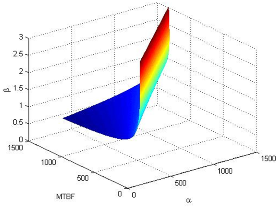
As shown in Figure 1, according to the curve of f(β) and y = [(S2 + M2)/M2], the surface of function β(M, S) can be drawn with intervals [ML, MU] and [SL, US]. According to equation (8) and by taking (M, β) as independent variables, the surface of function α (M, β) can be drawn, which is shown in Figure 2.
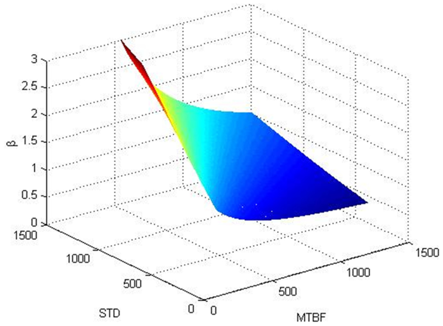
Surface of function β(M, S).
Surface of function α(M, β).
Figures 1 and 2 show that the extreme values of M and S determine the extreme values of β; the extreme values of M and β determine the extreme values of α. Therefore, according to the values (ML, SL), (MU, SL,), (ML, SU), and (MU, SU), the extreme values of α and β are determined and their intervals [αL, αU] and [βL, βU] can be obtained.
Prior distributions of Weibull parameters
Although [αL, αU] and [βL, βU] are obtained, the most possible value and the interaction between α and β have not been determined. According to Berger, 30 both α and β are uniformly and independently distributed. Therefore, the PDFs of α, β, and (α, β) are regarded as prior distributions
where α∈(αL, αU) and β∈(βL, βU).
Posterior distributions of Weibull parameters
The posterior distributions of Weibull parameters can be obtained through Bayes theorem. The prior distribution of
The marginal distribution of
π(
By taking the prior distribution, the likelihood function, and the marginal distribution of
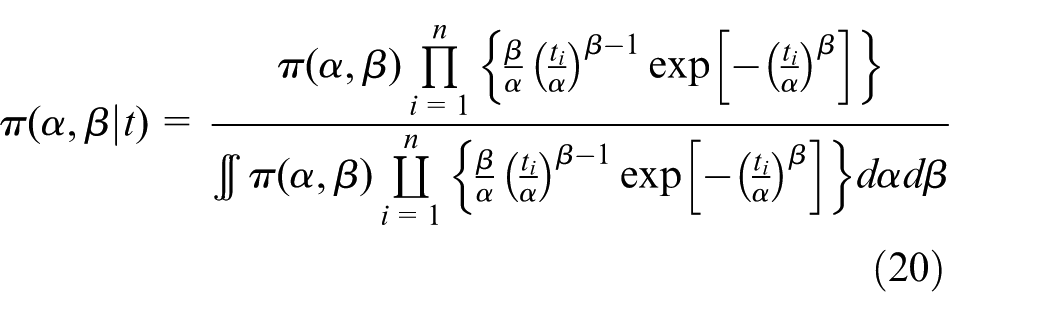
Equation (20) is complex and has no analytic solution. The Weibull parameters also have these characteristics. To solve this problem, the Markov chain Monte Carlo (MCMC) method is adopted to simulate the theoretical posterior distributions of α and β.31,32
Solving the posterior distributions of parameters
For
Given that equation (20) is too complex, the software WinBUGS is used to develop and conduct the MCMC method. By conducting the MCMC method, WinBUGS generates considerable simulated parameter values and provides a large number of statistics of the parameters automatically, which include the posterior mean values of α and β. To conduct the MCMC method in WinBUGS software, equation (20) should be rewritten as follows
The BUGS model of the target distribution is based on equation (23). An intact BUGS model includes three parts, namely, the prior distributions, the likelihood function, and the data. Each part needs to be described in BUGS language.
Comparison and verification
Two reliability tests are conducted on two batches of machining centers. In the reliability test on the first batch, a large data sample is collected and used to compare the traditional change point estimation method with the Bayes change point estimation method proposed in this study. When the Bayes method is verified, it is applied to the second batch of machining centers with a small data sample.
Obtaining failure data
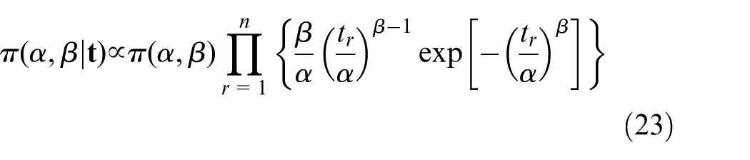
The first batch of machining centers includes seven products of the same model M1, which are denoted by V01, V02, …, V07. A total of 60 failure data points are obtained, as shown in Table 1.
Reliability test data of seven machining centers.
TBF: time between failures.
Solving the change point with the Bayesian method
According to the expert judgment procedure in section “Building the prior distributions of Weibull parameters,” M1 is taken as the reference NCMT, and V01, V02, …, V07 are taken as the target NCMTs in turn. The experts determine the value ranges of MTBF and STD based on the multi-source prior information, and their judgments are integrated into the final result as follows: [ML, MU] = [375, 702], [SL, US] = [549, 732]. Through equation (8), equation (15), and the transformation procedure in “Transforming expert judgment into prior distributions,” the extreme values of α and β are obtained as follows: αL = 221.99; αU = 758.75; βL = 0.55; βU = 1.29. The prior distributions of α and β are π(
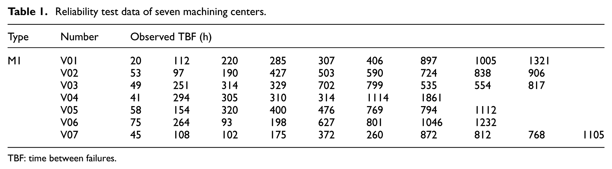
V01 is taken as the target NCMT, and the data samples of V01 corresponding to each failure, t1 = {20}, t2 = {20, 112}, t3 = {20, 112, 220} are taken into WinBUGS model. The corresponding βs are obtained by the MCMC method. As shown in Table 2, the sum of the observed TBFs in each data sample is the total working time of the NCMT, and β changes as the total working time increases. Therefore, β is taken as the function of the total working time, β(t). Table 2 shows that the total working time tc that satisfies β(t) = 1 can be worked out with the linear interpolation method, and tc is defined as the length of the early failure period of V01. The early failure period length of V02, …, V07 can be worked out in the same way, which is shown in Table 2.
Estimators of the beta of the first batch of machining centers with different data samples.
TBF: time between failures.
Cluster analysis to solve the change point
An earlier study 17 drew the bathtub curve with a non-parametric method based on a large data sample. The change point of the bathtub curve can then be obtained through the clustering analysis. 33 The detailed steps are as follows:
The observed yi (i = 1, 2, …, n) are rearranged in an ascending order. The rearranged data are divided into m intervals according to their values. The number kj (j = 1, 2, …, m) of the data points in each interval is counted.
t1 is used to represent the interval
3. The bathtub curve is drawn based on equation (24), as shown in Figure 3.
4. A partition point i = ic is needed to divide the data sample into two groups using the cluster method. The data in one group are close to another and are considerably different from those in the other group. The first group average µ1(i) and the second group average µ2(i) are given as follows
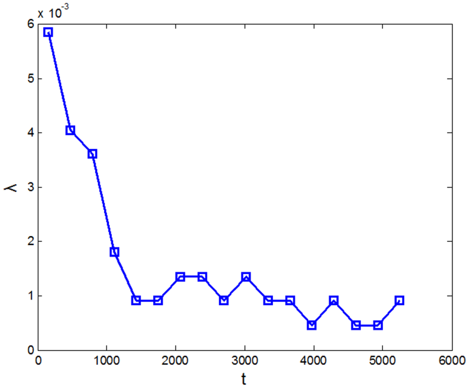
Empirical intensity function.
5. The “distance” between yi and the first (second) group is measured by

The “similarity” between yi and the first (second) group is measured by

The curves of S1 and S2 are drawn, as shown in Figure 4.
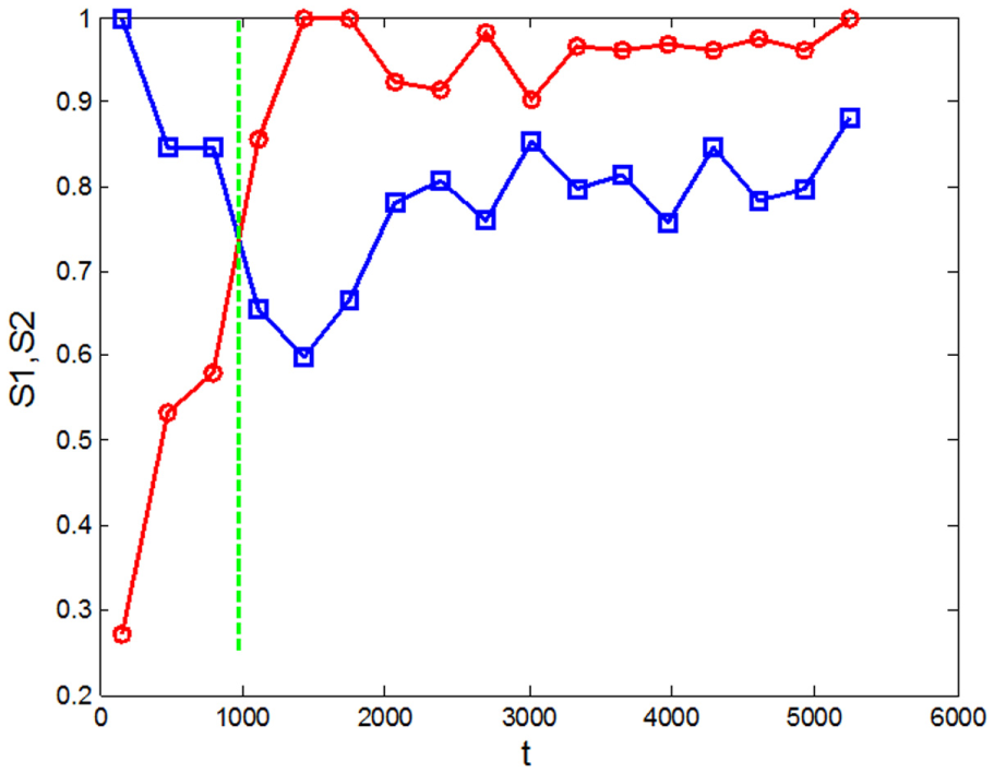
Plots of similarities for the change point.
7. Using linear interpolation, the estimate of tc is derived by
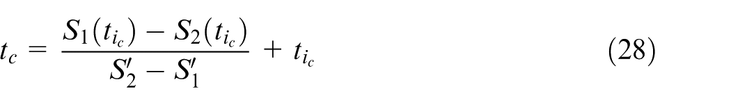
where
Through the six steps above, the change point of the first batch of machining centers can be solved; its value tc is 974.22 h.
The eighth column of Table 2 presents the estimated values of tc derived by the Bayesian method proposed by this study, in which the highest and lowest values of tc are 1062.68 and 843.67 h, respectively. The mean value of tc in the eighth column is 925.55 h, which is close to 974.22 h. The value is obtained through the clustering analysis and based on the large data sample. The distance between 925.55 and 974.22 h is 2 or 3 days. From the engineering perspective, this distance nearly has no influence on the economic interest of enterprises. The preceding comparison and discussion verify that the Bayes method based on small data sample proposed by this study can be the best way to estimate the early failure period when the traditional method is invalidated by the lack of data. The proposed Bayesian method is applied to a small data sample in the following section.
Example
Target machine tool
The reliability test is conducted on the second batch of machining centers from 26 October 2014 to 28 May 2015. This batch has only one machining center, and its model is represented by M2. During the test, five failures occur, as shown in Table 3.
Small-sample data of the target machining center.
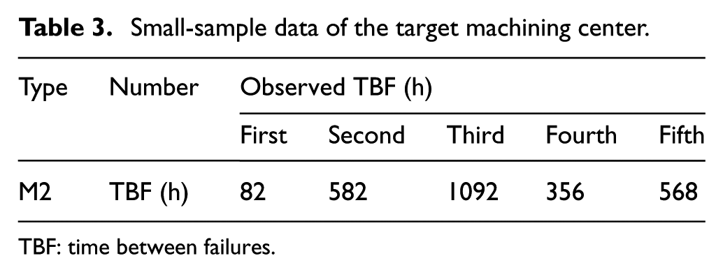
TBF: time between failures.
Prior distributions of Weibull parameters
According to the expert judgment procedure in section “Building the prior distributions of Weibull parameters,” an expert group composed of five experts is organized. Given that M2 is upgraded based on M1, we take M1 as the reference machining center. Then, the value ranges of MTBF and STD are [415.64, 628.08] and [359.61, 604.86], respectively, with the significance level 0.05.
According to the data above and the multi-source prior information of M1, the five experts give the value ranges of MTBF and STD about M2, as shown in Table 4.
Results of expert judgment.
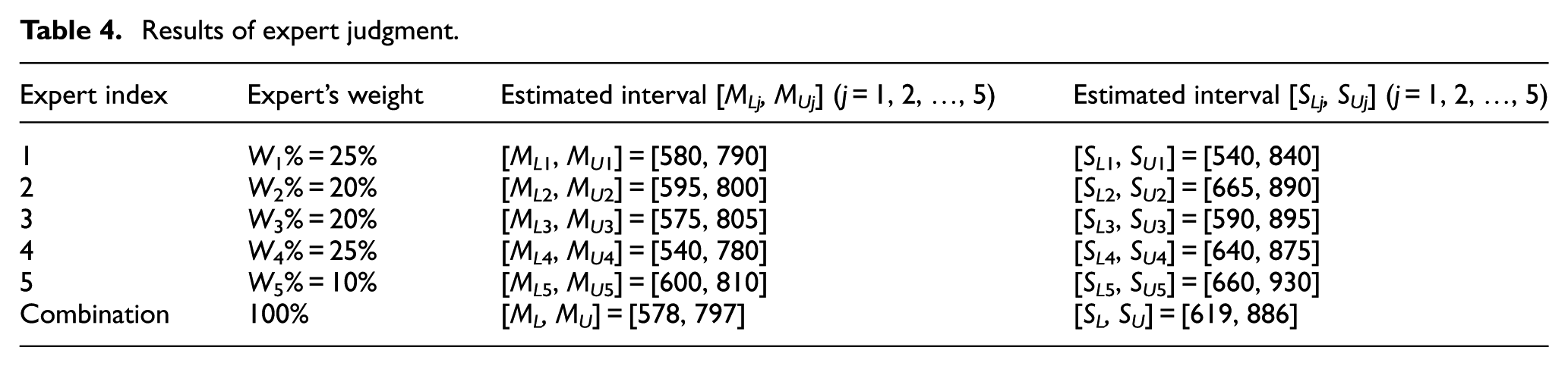
According to the transformation method in section “Transforming expert judgment into prior distributions,” (ML, MU) and (SL, SL) are transformed into intervals (αL, αU) = (447.3984, 862.7213), (βL, βU) = (0.6855, 1.2983). Assume that α and β are independently and uniformly distributed in the corresponding intervals; then, the prior distribution of the parameter vector is π(
Posterior distributions of Weibull parameters
Based on equation (23), the MCMC method is conducted in WinBUGS to simulate the posterior distributions derived using equation (20). To make the estimation accurate, three Markov chains are generated in WinBUGS, and the iteration number of each parameter is set as 10,000.
First, the WinBUGS model is established with the first data sample t1 = 82 h. The statistics of α and β given by the MCMC method are shown in Table 5.
Posterior statistics obtained by MCMC simulation in WinBUGS.
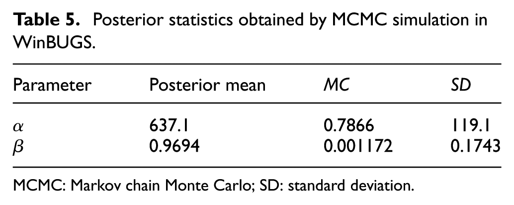
MCMC: Markov chain Monte Carlo; SD: standard deviation.
From Table 5, the following equations can be obtained: MCα = 0.7866<SDα×5% = 119.1×5% = 5.955; MCβ=0.001172<SDβ×5%=0.1743×5%=0.008715.
The MC values of α and β are all less than 5% of SD. Therefore, the calculation results are accepted. In other words, the estimations of the posterior distributions of α and β are good.
The iteration processes of the dynamic simulation are shown in Figures 5 and 6.
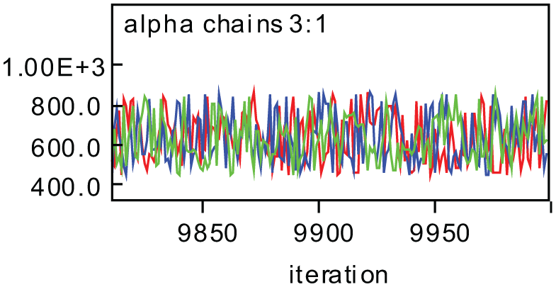
Iteration processes of α.
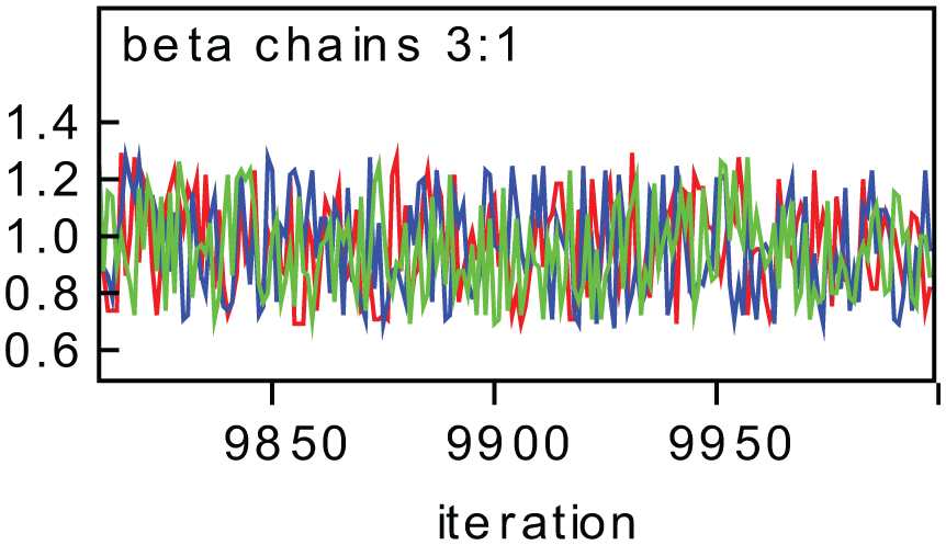
Iteration processes of β.
Figures 7 and 8 present the nuclear density curves of α and β, where the first 500 simulation values are abandoned as burning-in data. The remaining 9500 simulation values are used to simulate the posterior PDFs of α and β.
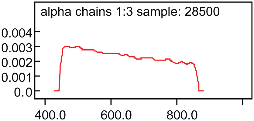
Nuclear density curves of α.
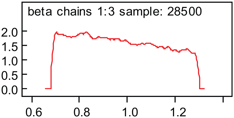
Nuclear density curves of β.
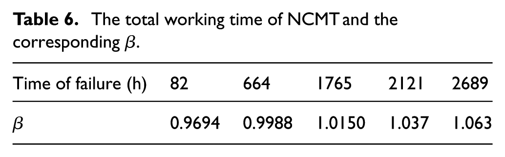
β2 = 0.9988 is obtained with the MCMC method based on the WinBUGS model, which is built by the first two data (t1 = 82 h, t2 = 582 h). The other estimation values of β can be worked out in the same way, based on the first three, first four, and first five data, which are shown in Table 6.
The total working time of NCMT and the corresponding β
Solving the change point
According to Table 6 and by taking β as the function of the total working time t, the total working time that satisfies β(t)=1 can be derived easily with the linear interpolation method; the result is tc=715.56 h. tc = 715.56 h is regarded as the early failure period of M2. Therefore, the Bayesian method proposed in this study can estimate the early failure period of NCMT with a few machines and less time.
Conclusion
This study proposes a Bayesian method to estimate the early failure period of NCMT with a small data sample, based on the reliability model of NCMT conforms to the two-parameter Weibull distribution. By taking the Weibull shape parameter β as the function of time t, we obtain the total working time that satisfies β(t)=1 as the change point of the bathtub curve. The conclusions are as follows:
An expert judgment procedure, which integrates the multi-source prior information of NCMT and the reliability test data of the reference NCMT, is designed and applied. The judgment result is transformed into the prior information of the Weibull parameters. The expert judgment procedure can avoid the subjective bias and significantly promote the accuracy of the modeling.
The cluster analysis method is applied to a large data sample of machining center with type M1, working out the early failure period as 974.22 h. The method proposed by this study is applied to the small data sample of M1, working out the mean value of the early failure period as 925.55 h. Comparison shows that the estimation result of the proposed Bayesian method with a small data sample is close to that of the classic method with a large data sample, and the error can be omitted from the engineering perspective.
The early failure period of M2, which is upgraded from M1, is obtained by the Bayesian method and the result is 715.56 h. The result of the comparison between M1 and M2 shows that the early failure period decreases with the improvement of the NCMT. This method can be used to guide the early failure test and to design rational maintenance strategies in different failure periods, which are of vital significance.
Footnotes
Declaration of conflicting interests
The author(s) declared no potential conflicts of interest with respect to the research, authorship, and/or publication of this article.
Funding
The author(s) disclosed receipt of the following financial support for the research, authorship, and/or publication of this article: This project (2014ZX04014-011) was supported by State Key Science & Technology Project: Research on the Reliability Assessment and Test Methods of Heavy Machine Tools.