Sage Journals: Discover world-class research

Abstract

Angular distortion in fusion welded joints is an alarming issue which affects the stability and life of the welded structures, occurs due to the changes in the temperature gradient during the welding process. This degrades the dimensional quality of a large structure during assembly which leads to rework the products and hence decreases the productivity. Predicting the weld-induced residual deformation before the production saves the valuable time and resources for rework. The conventional coupled transient, nonlinear, elasto-plastic thermo-mechanical analysis involves huge computational time. Computing a weld sample of small size with single pass itself takes several hours, which will be a huge amount of time in case of large structures consisting of several welding passes; thus, there is a real need of an efficient alternative technique to predict the post-weld distortions. In this work, an attempt has been made to determine the deformation in a submerged arc welded structure using equivalent load technique which reduces the total analysis time by one-third of the conventional techniques in case of a small weld structure. In this proposed method, the transient nonlinear elasto-plastic structural analysis part which is the major time-consuming part of analysis has been almost eliminated. So, this method can effectively use to predict the weld-induced distortion of very large structure with a computation time almost equal to the time required for transient thermal analysis of a small weld structure only. It is not feasible to analyze such a large welded structure with conventional coupled transient, elasto-plastic, nonlinear thermo-mechanical analysis. The predicted results of distortions have been validated with the experimental as well as published results and good agreements have been found.

Keywords

Equivalent loading technique finite element model distortion large structure submerged arc welded

Introduction

The arc welding process is a very complex phenomenon involving extremely high temperature gradients, leading to micro-structural changes and formation of thermal stresses.¹ These stresses may cause distortions and produce high levels of residual stresses. These tend to reduce the strength of the structure, which becomes vulnerable to fracture, buckling, and fatigue and may suffer enhanced corrosion. The problem of distortion during fabrication process leads to dimensional inaccuracies and misalignments of structural members, which may require corrective tasks or rework if tolerance limit is exceeded. This, in turn, lengthens the production cycle leading to increase in the cost of production. Hence, the problem of distortion and residual stresses are always of great concern in shipbuilding industries.

To deal with this problem, suitable mitigation techniques are to be developed. However, prior to that, it is necessary to have a reliable prediction tool to assess the extent of possible distortion and residual stresses that may form during fabrication. During welding, there are various factors such as welding parameters, welding sequence, heating and cooling patterns, level of constraints, and joint details which influence the extent of distortion and residual stress.

Understanding the theory of heat flow is essential to study the welding process. The first research was done by Rosenthal² in the development of an analytical solution of heat flow during welding based on conduction heat transfer for predicting the shape of weld pool for two-dimensional (2D) and three-dimensional (3D) welds. He introduced the moving coordinate system to develop solutions for point and line heat sources during welding. His analytical solution of heat flow helped in analyzing the problem taking current, voltage, welding speed, and weld geometry into consideration. Goldak et al.³ derived a mathematical model for welding heat source based on Gaussian distribution of power density. They proposed double ellipsoidal distribution in order to capture the shape and size of the heat source for shallow and deeper penetrations. Watanabe and Satoh⁴ used analytical methods resulting from the theory of elasticity for prediction of thermal deformations during welding and line heating. However, since elastic solutions are limited, application of this method is also limited. Ueda and Yamakawa⁵ were the first among those who analyze the transient thermal stresses using thermal elasto-plastic finite element model (FEM) in a butt joint configuration with considering material deposition from a moving electrode. Following this pioneering work, many researchers have successfully developed various numerical models^6–12 based on finite element (FE) method to predict temperature distribution, analyze the welding residual stress and distortion both in 2D and 3D problems. Tekriwal and Mazumdar¹³ and Bonifaz¹⁴ developed thermal FE simulations to investigate the temperature distribution of metals. Over a sustained period of time, finite element analysis (FEA) is used by many researchers to predict the temperature distribution, residual stresses and distortion of welded joints. Prominent among them are Friedman,¹⁵ Brown and Song¹⁶ and Michaleris and Debiccari.¹⁷ Use of FEA has been successful in predicting temperature distribution, distortion, and also in tackling of complex phenomena like crack propagation in welded joints. Many researchers used 2D FEA of Friedman¹⁵ to verify their 3D computational model of welding process. Most of the welding research in the past was carried out to investigate the distribution of residual stress and distortion of welded metal. The work performed by Mandal and Sundar¹⁸ estimates the welding shrinkage in a welded butt joint by applying a near field–far field approach. Michaleris and Debiccari¹⁷ conducted thermo-elasto-plastic FEA to predict distortion during welding. Puchaicela¹⁹ reviewed and analyzed several formulae in an attempt to provide a practical guide to control and reduce distortion. Biswas et al.²⁰ and Biswas and Mandal²¹ performed numerical study to estimate the residual stress and angular deformation in fillet and butt joints which was validated by experimental data. Along with numerical study, some researchers did experimental study to determine the effect of different process parameters;²² few of them worked to optimize the process parameters for getting the target weld quality.^23,24

In addition to residual stresses and distortion, researchers have also studied the effect of welding parameters, welding sequences, welding joint geometry, and root opening in the past. Tsai et al.²⁵ studied the effect of welding sequence on buckling and warping behavior of a thin plate panel structure. Tsai et al.²⁶ have also investigated the effect of welding parameters and joint geometry on the magnitude and distribution of residual stresses on thick section butt joint.

Some recent studies were performed to analyze the molten pool behavior²⁷ and to determine the influence of activated flux on mechanical properties.^28,29 Effect of heat input on weld bead geometry³⁰ and influence of process variables on the quality of weld was studied by Kiran et al.³¹ Several researchers^32,33 have done extensive study on the analysis of microstructure of submerged arc welded (SAW) steel joints. The effect of root opening on the mechanical properties, deformations, and residual stress is investigated by Jang et al.³⁴ FEA of residual stresses in case of butt weld is reported by Hong et al.³⁵

Cho et al.³⁶ have reported detailed analysis on the determination of residual stress distribution after welding and after a post-weld heat treatment using a FE transient heat flow analysis in conjunction with a coupled thermo-mechanical analysis. A 3D FEM was developed by Mahapatra et al.³⁷ to predict the effect of SAW process parameters on temperature distribution and angular distortions in single-pass butt joints with top and bottom reinforcements (to minimize angular distortions). The process was modeled considering a distributed moving heat source, reinforcements, filler material deposition in each pass of welding, and temperature-dependent material properties.

But problem with these models is the huge time consumption for structural analysis. Some researchers tried to develop various equivalent techniques to minimize the analysis time. Souloumiac et al.³⁸ developed a local/global approach in order to determine the welding residual distortions of large structures. They assumed that plastic strains induced during welding process were located close to the welding path and depend on local thermal and mechanical conditions. The plastic strains obtained by the local approach were then projected to a complete shell of whole structure as initial strain. The final distortions were computed using an elastic simulation.

Ueda et al.³⁹ proposed the experiment-based, equivalent-mechanical-loading method to obtain the final deformation quickly. It assumes that the assigned mechanical forces and moments adjacent to weld joints generate welding deformation. A critical limitation of this method was that the applied loads should be calculated only from experiments. To overcome this limitation, Murakawa et al.⁴⁰ proposed the inherent strain-based, equivalent-mechanical-loading method. Many researchers further developed this methodology and applied it to predict welding distortion.⁴¹ However, this methodology also had limitations when applied to welded structures with curved welding joints, because the imposed forces might induce welding shrinkage, as well as unexpected angular distortion while dealing with a curved weld line. Ha⁴² and Ha et al.⁴³ had suggested that an inherent strain-based, equivalent-thermal-loading method by which the combination of nodal temperatures and imaginary thermal expansion coefficient (α) could induce welding deformation. They assumed that the positive temperature values are assigned into certain weld line nodes, and others are zero. Also, the imaginary, negative thermal expansion coefficient values equivalent to the inherent strain (ε*) for the joint of concern are mapped only onto the weld line elements. The philosophy of this simplified analysis methodology is that the final welding deformation can be produced by FEA, after thermally loaded elements close to the weld line are subjected to elasto-plastic behavior by surrounding a stiffened region with no temperature change.

This article presents an efficient FE technique using equivalent load to precisely predict welding deformations and residual stresses in large structures. Equivalent load method is based on inherent strains which are a function of the highest temperature and degree of restrain. Nonlinear FE transient thermal analysis is performed using surface heat source model with Gaussian distribution to compute the temperature distribution in mild steel (MS) plates. Equivalent loads are calculated using the inherent strain components. An elastic FE analysis of weldment using these equivalent loads is performed to simulate deformation and residual stresses. Predicted distortions show a good agreement with the experimental measurements/published results, and the total computation time was reduced, which proves the reliability of the proposed technique.

Experimental investigation

Submerged arc welding is an automatic welding technique where the consumable electrode is continuously fed by a wire feeding mechanism toward the weld line at a controlled rate and the welding torch is moved automatically along the weld seam. The heat generated by the arc progressively melts the electrode tip, the adjacent edges of base metal and some of the flux, which is continuously fed in front and around the electrode from a hopper. The molten slag, thus formed, floats on the molten metal and thus completely shields the molten pool from atmospheric contamination.

As the welding arc advances along the seam, the deposited weld metal and the liquid slag cools down and solidifies, forming the weld bead and the protective slag shield over it. This slag shield results in a slower cooling rate for the deposited weld metal, thus providing an annealing effect to the weld deposit. In the present investigation, welding was carried out using ESAB automatic submerged arc welding set up where voltage, current, welding speed, and length of stick out can be controlled. Wire feed was automatically controlled with welding speed. Solid granulated fusible flux was used as shielding medium for MS. Copper-coated MS filler wire of 3.15 mm diameter was used during welding of commercial grade MS samples.

To improve the bottom reinforcement, an aluminum backing bar was placed below the weld region along the root of a weld joint to support molten weld metal. The experimental setup is shown in Figure 1.

Figure 1.

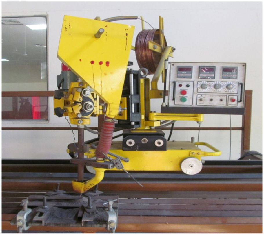
Experimental setup.

The temperature during welding is measured using K-type thermocouples. The thermocouples were connected to AGILENT 34972A data logger device with 20 channels multiplexer. This data logging device is connected to a PC and the temperature at different locations is measured with time. The angular distortions are measured using a coordinate measuring machine (CMM). Before welding, the tack-welded samples were marked to measure the coordinates before and after welding with respect to a reference surface. The angular distortion is calculated by subtracting the initial welded sample surface height from the final welded sample surface height.

Numerical model

A 3D FE model was developed in this work to perform the thermal as well as structural analysis in SAW MS samples.

Thermal modeling

From the literature survey, it is clear that heat transfer mechanism in molten pool is extremely complex and its physics is not well understood. Although some progress has recently been made toward the proper modeling of convective heat transfer, these efforts are still directed toward simple cases. Various material properties of the metals in the molten state are also not authentically established. In arc welding, except a small volume of metal, most of the portion of the work-piece remains in solid state. Therefore, a 3D conduction model was developed to analyze the heat transfer in all portions of the workpiece.

Assumptions in thermal model

To develop the thermal model, it is required to implement the actual welding condition as far as possible. Some assumptions are made to develop the thermal model of the welding process. The thermal properties are assumed to be the function of temperature. Density of MS was kept constant as 7850 kg/m³ for all temperatures. Linear Newtonian convection cooling was considered on all the surfaces except the weld zone without any forced convection. Radiation loss was also omitted which is compensated by introducing arc efficiency. Heat flux was applied as load.

Formulation of 3D FEA model of heat transfer in arc welding

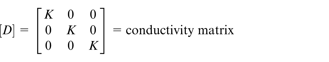
The Fourier law⁴⁴ is used as the governing equation for heat conduction for a homogenous, isotropic solid without heat generation in rectangular coordinate system (x, y, z) as follows

\frac{\partial}{\partial x} [k \frac{\partial T}{\partial x}] + \frac{\partial}{\partial y} [k \frac{\partial T}{\partial y}] + \frac{\partial}{\partial z} [k \frac{\partial T}{\partial z}] = ρ c \frac{\partial T}{\partial t}

(1)

Equation (1) can be written as

ρ c \frac{\partial T}{\partial t} = - {L}^{T} {q}

(2)

where

${L}^{T} T = \vec{\nabla} T$ and ${L}^{T} {q} = \vec{\nabla} \cdot {q}$

{L} = {\begin{matrix} \frac{\partial}{\partial x} \\ \frac{\partial}{\partial y} \\ \frac{\partial}{\partial z} \end{matrix}} = vector operator

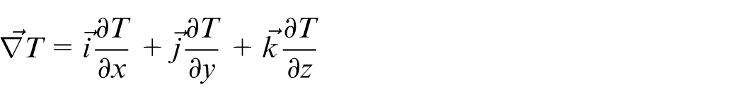
Fourier’s law is used to relate the heat flux vector to the thermal gradient

{q} = - [D] {L} T

where

[D] = [\begin{matrix} K & 0 & 0 \\ 0 & K & 0 \\ 0 & 0 & K \end{matrix}] = conductivity matrix

Equation (2) can be written as follows

ρ c \frac{\partial T}{\partial t} = {L}^{T} ([D] {L} T)

(3)

Boundary conditions

Initial condition 1

An initial temperature is considered for the entire elements of the specimen as follows

T = T_{\infty} for t = 0

(4)

where $T_{\infty}$ is the ambient temperature. $q_{\sup}$ represents the heat flux supplied to the work surface in W/m² from an external welding arc. $q_{conv}$ represents the heat loss from the work surface at temperature, T by convection with a heat transfer coefficient, h_f into an external ambient temperature. $q_{conv}$ can be represented as follows

q_{conv} = h_{f} (T - T_{\infty})

(5)

It should be noted that heat flux, $q_{\sup}$ , and convection loss, $q_{conv}$ , do not occur over the same boundary segment. If heat loss by convection exists, then heat gain by $q_{\sup}$ does not or vice versa.

Let $\vec{n}$ is the unit outward normal vector represented as $\vec{n} = \vec{i} l_{x} + \vec{j} l_{y} + \vec{k} l_{z}$ .The quantity, $q_{n}$ , represents the component of the conduction heat flux vector normal to the work surface and it is given as follows

q_{n} = - K \vec{\nabla} T \cdot \vec{n}

(6)

where

\vec{\nabla} T = \vec{i} \frac{\partial T}{\partial x} + \vec{j} \frac{\partial T}{\partial y} + \vec{k} \frac{\partial T}{\partial z}

The normal component of the heat flux vector at the surface becomes

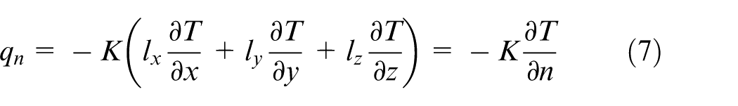
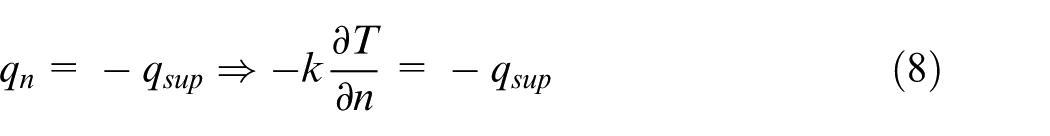
q_{n} = - K (l_{x} \frac{\partial T}{\partial x} + l_{y} \frac{\partial T}{\partial y} + l_{z} \frac{\partial T}{\partial z}) = - K \frac{\partial T}{\partial n}

(7)

To develop the second and third boundary conditions, the energy balance considered at the work surface as, heat supply = heat loss.

Boundary condition 1

A specific heat flow acting over surface S₁ as follows

q_{n} = - q_{\sup} \Rightarrow - k \frac{\partial T}{\partial n} = - q_{\sup}

(8)

Boundary condition 2

Considering heat loss due to convection over surface S₂ (Newton’s law of cooling)

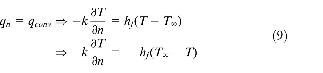
q_{n} = q_{c o n v} \Rightarrow - k \frac{\partial T}{\partial n} = h_{f} (T - T_{\infty}) \Rightarrow - k \frac{\partial T}{\partial n} = - h_{f} (T_{\infty} - T)

(9)

Note that positive specified heat flow is into the boundary (i.e. in the direction opposite of $\vec{n}$ ). Pre-multiplying equation (3) by a virtual change in temperature, integrating over the volume of the element, and combining with equations (8) and (9) with some manipulation yield

\begin{matrix} \int_{vol} (ρ c δ T (\frac{\partial T}{\partial t}) + {L}^{T} (δ T) ([D] {L} T)) d (vol) \\ = \int_{s_{1}} δ T q_{\sup} d (S_{1}) + \int_{s_{2}} δ T h_{f} (T_{\infty} - T) d (S_{2}) \end{matrix}

(10)

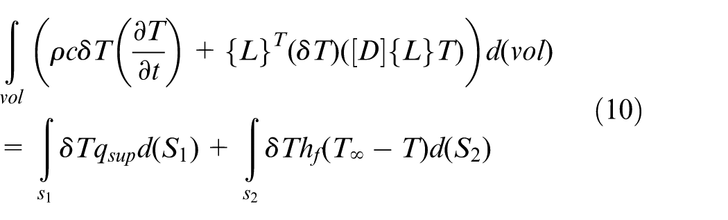
where vol = volume of element and δT = an allowable virtual temperature (= δT(x, y, z, t)).

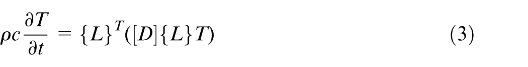
Derivation of heat flow matrices

As stated before, the variable T was allowed to vary both in space and time. This dependency is expressed as follows

T = {N}^{T} {T_{e}}

(11)

where $T = T (x, y, z, t) = temperature$ , ${N} = {N (x, y, z, t)} = element shape function$ , and ${T_{e}} = {T_{e} (t)} = nodal temperature vector$ . Thus, the time derivatives of equation (11) may be written as follows

\overset{\cdot}{T} = \frac{\partial T}{\partial t} = {N}^{T} {\overset{\cdot}{T} e (t)}

(12)

where $δ T$ has the same form as T

δ T = {δ T_{e}}^{T} {N}

(13)

The combination of ${L} T$ is written as ${L} T = [B] {T_{e}}$ , where

[B] = {L} {N}^{T}

(14)

Now, equation (10) can be combined with equations (11)–(14) to yield

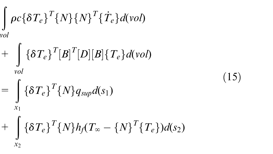
\begin{matrix} \int_{vol} ρ c {δ T_{e}}^{T} {N} {N}^{T} {{\overset{\cdot}{T}}_{e}} d (vol) \\ + \int_{vol} {δ T_{e}}^{T} {[B]}^{T} [D] [B] {T_{e}} d (vol) \\ = \int_{x_{1}} {δ T_{e}}^{T} {N} q_{\sup} d (s_{1}) \\ + \int_{x_{2}} {δ T_{e}}^{T} {N} h_{f} (T_{\infty} - {N}^{T} {T_{e}}) d (s_{2}) \end{matrix}

(15)

The density $ρ$ is assumed to remain constant and specific heat c may vary over the element. Finally, ${T_{e}}, {{\overset{\cdot}{T}}_{e}}, {δ T_{e}}$ are nodal quantities and do not vary over the element, hence may be neglected from the integrals. Now, since all quantities are seem to be pre-multiplied ${δ T_{e}}$ , this term may also be dropped from the resulting equation. Thus, equation (15) may be reduced to

\begin{matrix} ρ \int_{vol} c {N} {N}^{T} d (vol) {{\overset{\cdot}{T}}_{e}} + \int_{vol} {[B]}^{T} [D] [B] d (vol) {T_{e}} \\ = \int_{x_{1}} {N} q_{\sup} d (s_{1}) + \int_{x_{2}} T_{\infty} {N} h_{f} d (s_{2}) \\ - \int_{s_{2}} h_{f} {N} {N}^{T} {T_{e}}) d (s_{2}) \end{matrix}

(16)

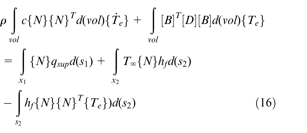
Equation (16) can be written as

[C_{e}^{t}] {{\overset{\cdot}{T}}_{e}} + ([K_{e}^{tb}] + [K_{e}^{tc}]) {T_{e}} = {Q_{e}^{f}} + {Q_{e}^{c}}

(17)

where $[C_{e}^{t}] = ρ \int_{vol} c {N} {N}^{T} d (vol)$ is the element-specific heat matrix; $[K_{e}^{tb}] = \int_{vol} {[B]}^{T} [D] [B] d (vol)$ is the element conductivity matrix; $[K_{e}^{tc}] = \int_{S_{2}} h_{f} [N] {[N]}^{T} d (S_{2})$ is the element convective matrix; ${Q_{e}^{f}} = \int_{S_{1}} {N} q_{\sup} d (S_{1})$ is the element heat flow vector; and ${Q_{e}^{c}} = \int_{S_{2}} T_{\infty} h_{f} {N} d (S_{2})$ is the element heat flow vector.

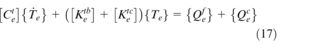
The thermo-mechanical analysis of 3D FE model was solved using ANSYS 14.0 package.

Transient heat flow analysis

The distribution of heat applied on the surface of the work-piece or in a volume internal to the weldment has an important effect on the heat distribution pattern in the vicinity of the weld. In this region, weld bead and heat-affected zone (HAZ) are formed. It is important to identify that how the heat input distribution influences their size and shape, if the weld thermal cycle in the vicinity of the weld metal and HAZ is not of interest. The heat input distribution is not important, and the heat input can be treated as a concentrated heat source. The heat input and the weld speed are then sufficient to determine the thermal cycle.

In the present case of submerged arc welding, the heat deposition was considered as a normally distributed heat flux on the weld surface. The net heat supplied is given by

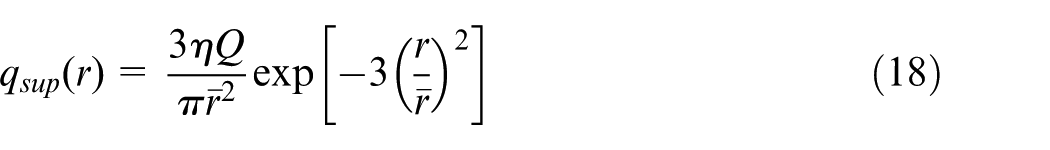
q_{\sup} (r) = \frac{3 η Q}{π {\bar{r}}^{2}} \exp [- 3 {(\frac{r}{\bar{r}})}^{2}]

(18)

where r is the distance from the center of the heat source on the surface, $\bar{r}$ is the characteristics radial dimensional distribution parameter that defines the region in which 95% of heat flux is deposited.¹⁵ $η$ is the welding efficiency, and Q is the power density, Q = VI = power, where V = voltage and I = current.

In this study, a moving was used for modeling the welding process. The total arc heat input to the joint can be applied as a volumetric moving heat source or as a surface heat flux input.⁴⁵ The heat flux can also be applied as a rectangular or square shape. In this work, the heat flux is applied on a square area.

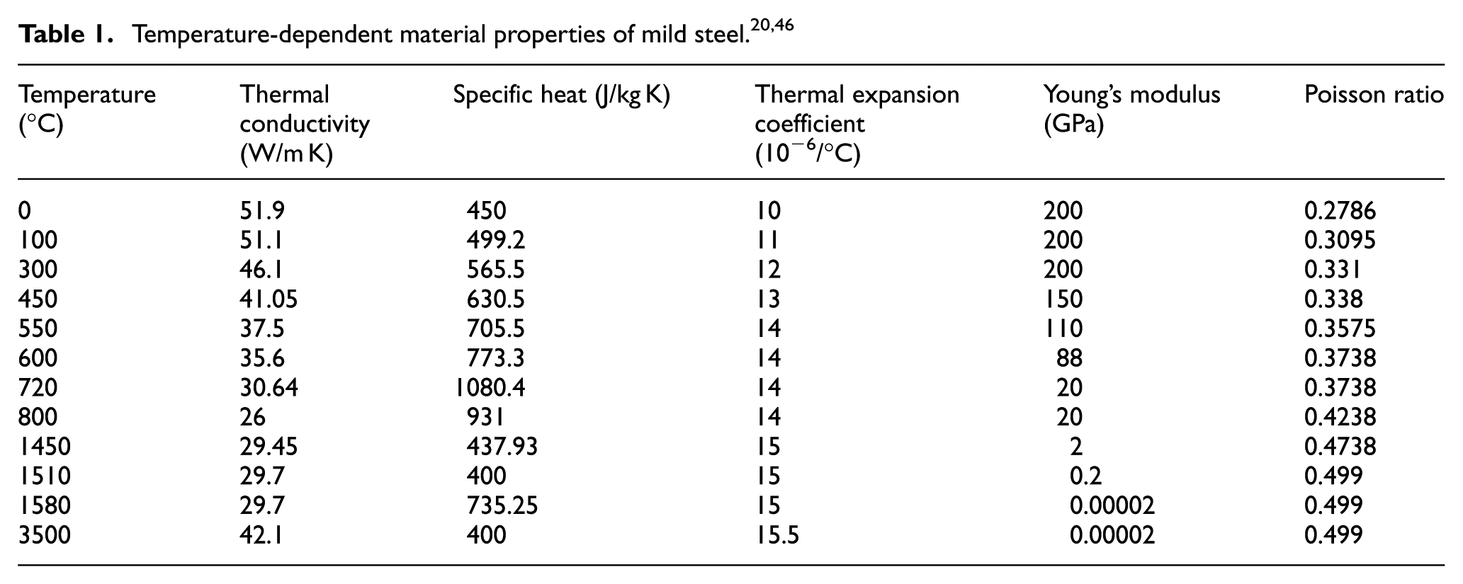
Material properties

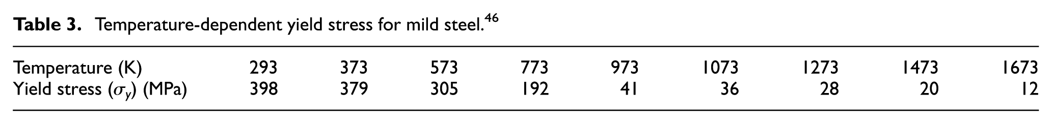
Both the weld plate and electrode were made of MS; hence, the temperature-dependent material properties of MS used for the transient heat transfer analysis and elasto-plastic analysis are given in Table 1. Temperature-dependent enthalpy and yield stress for MS are given in Tables 2 and 3, respectively. The melting and transformation temperature of MS are 1495 °C and 723 °C, respectively.

Table 1.

Temperature-dependent material properties of mild steel.^20,46

Temperature (°C)	Thermal conductivity (W/m K)	Specific heat (J/kg K)	Thermal expansion coefficient (10⁻⁶/°C)	Young’s modulus (GPa)	Poisson ratio
0	51.9	450	10	200	0.2786
100	51.1	499.2	11	200	0.3095
300	46.1	565.5	12	200	0.331
450	41.05	630.5	13	150	0.338
550	37.5	705.5	14	110	0.3575
600	35.6	773.3	14	88	0.3738
720	30.64	1080.4	14	20	0.3738
800	26	931	14	20	0.4238
1450	29.45	437.93	15	2	0.4738
1510	29.7	400	15	0.2	0.499
1580	29.7	735.25	15	0.00002	0.499
3500	42.1	400	15.5	0.00002	0.499

Table 2.

Temperature-dependent enthalpy for mild steel.⁴⁶

Temperature (°C)	0	100	200	300	400	500	600	700	800	900	1000	>2500
Enthalpy (MJ/m³)	0	360	720	1100	1500	1980	2500	3000	3700	4500	5000	9000

Table 3.

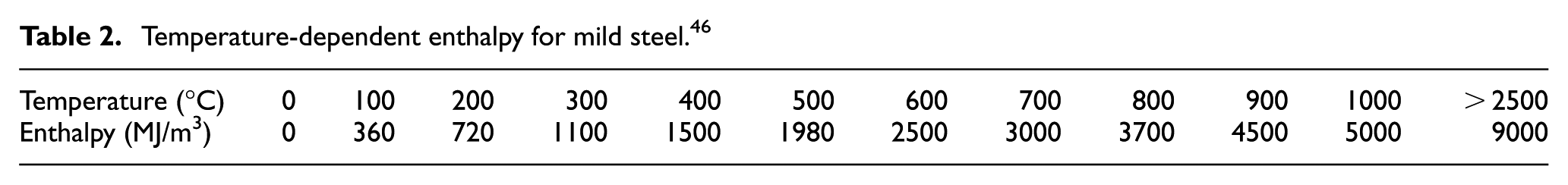
Temperature-dependent yield stress for mild steel.⁴⁶

Temperature (K)	293	373	573	773	973	1073	1273	1473	1673
Yield stress (σ_y) (MPa)	398	379	305	192	41	36	28	20	12

Thermal history of square butt welding

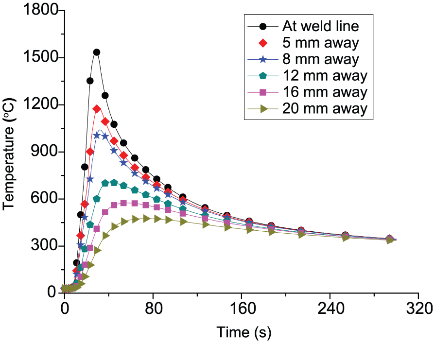
For FE modeling, eight-noded brick element is considered with fine meshing in the weld zone and coarse meshing away from the weld zone. In the thermal model, the deposition of filler material in the root gap is implemented using element death and birth technique. Free convection is applied on all the surfaces of the plates except weld region. The temperature distribution with time at various points on top and bottom surface of the square butt welded plate (10 mm thick) are shown in Figures 2 and 3, respectively. The value of the welding parameters considered during simulation is given in Table 4.

Figure 2.

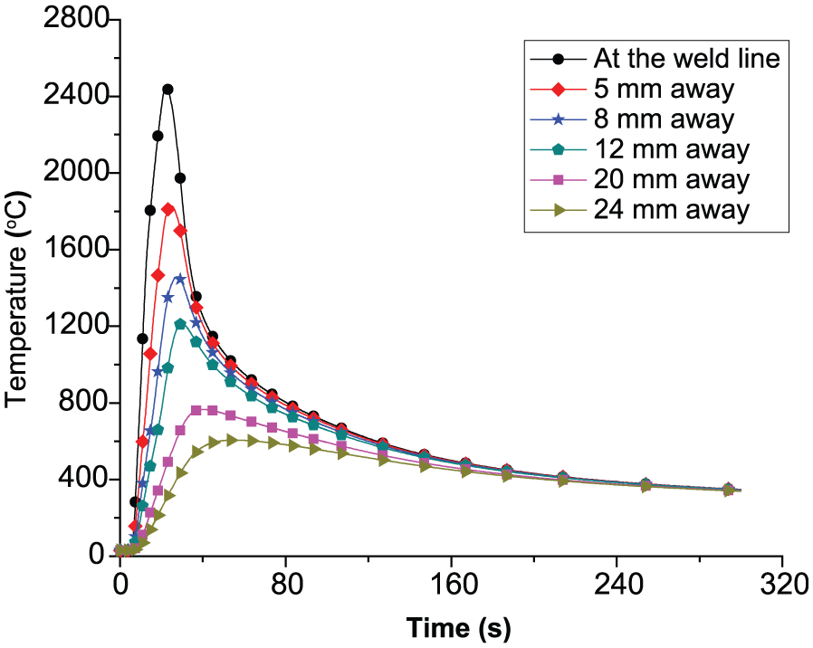
Temperature distribution at different distances away from the weld line on the top surface of the welded plate.

Figure 3.

Temperature distribution at different distances away from the weld line on the bottom surface of the welded plate.

Table 4.

Welding parameters considered for simulation.

Plate thickness (mm)	Welding parameters
	Current (A)	Voltage (V)	Speed (mm/s)
10	520	28	5.2

From Figures 2 and 3, it is observed that the peak temperature along the weld line is very high and as we move away from the weld line, the temperature decreases. In the welded zone, the peak temperature rises beyond the melting point temperature of MS which implies melting takes place in this zone (Figure 2). Also, it is observed that the temperature on the bottom surface is lower than the top surface at the same location.

Time temperature history captured by K-type thermocouple and data acquisition system is plotted in Figures 4 and 5. It can be observed that the trend of the experimental thermal history is well matching with the predicted one.

Figure 4.

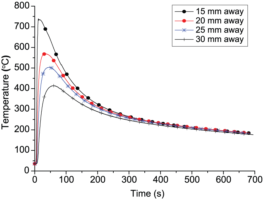
Temperature distribution at different distances away from the weld line on the top surface of the butt welded plate.

Figure 5.

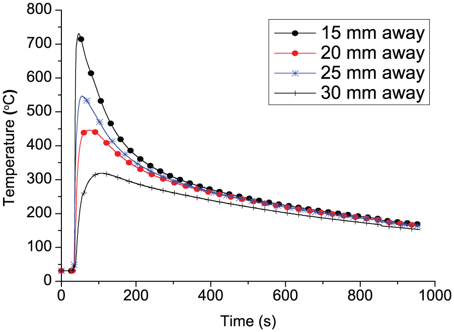
Temperature distribution at different distances away from the weld line on the top surface of the fillet welded plate.

Equivalent loading technique

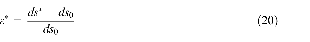
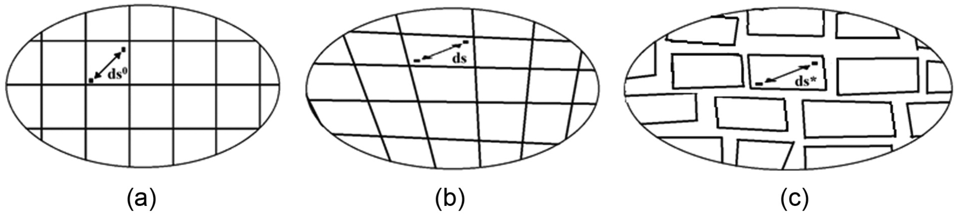
Let us consider a continuous body at different states that is (a) standard, (b) stressed, and (c) stress released as shown in Figure 6(a)–(c), respectively.⁴⁷ State (a) is the initial stress-free state where neither external force nor internal stress exists. This state is regarded as the standard state. State (b) is the residual stress. State (c) is the stress released state in which the body is cut into small elements. From state (b) to state (c), each element deforms elastically to completely release the residual stress. The distance between two close particles in the body is ds₀ in state (a), ds in state (b), ds* in state (c). The strain in the states (b) and (c) can be defined as shown in equations (19) and (20), respectively^48,49

ε = \frac{ds - d s_{0}}{d s_{0}}

(19)

ε^{*} = \frac{{ds}^{*} - d s_{0}}{d s_{0}}

(20)

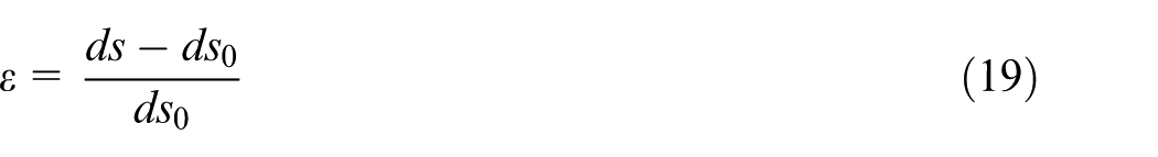
Similarly, the strain increment between states (b) and (c) can be defined as follows

ε^{e} = \frac{ds - {ds}^{*}}{d s_{0}}

(21)

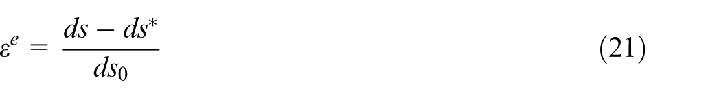
The strain defined in equation (19) is usually called total strain and it satisfies compatibility conditions. The strain defined in equation (20) is inherent strain and it does not follow compatibility conditions. The strain defined in equation (21) is elastic strain. The total strain is composed of elastic and inherent strains as in equation (22)

ε = ε^{e} + ε^{*}

(22)

Since the total strain, ε corresponds to the deformation and the elastic strain, ε^e corresponds to the stress, the above equation can be written as follows

ε^{*} = ε - ε^{e}

(23)

Hence, the inherent strain produces both the deformation (inherent deformation) and the residual stress.

Figure 6.

Inherent strain: (a) standard state, (b) stressed state, and (c) stress released state.^47,48

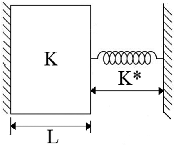
Inherent strain

The inherent strain occurs in the welded region and this region can be modeled as a bar. Its adjacent region resists deformation and it can be modeled as a spring as shown in Figure 7. The change in temperature in bar is much higher than that in the spring which acts as a restraint on the bar. The coefficient of restraint (β) can be written as

β = \frac{k^{*}}{k + k^{*}}

(24)

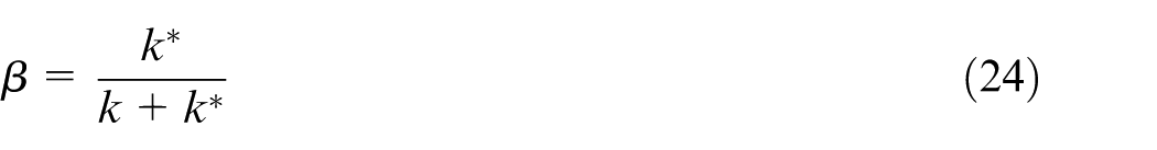
where k (= AE/L) is the stiffness of the bar, k* is the stiffness of the spring, A and L are the cross-sectional area and the length of the bar, respectively.

Figure 7.

Simplified elastic-plastic analysis model.⁵⁰

The inherent strain can be calculated as follows

ε^{*} = \frac{- ε_{Y}}{β} = \frac{- σ_{Y}}{E β}

(25)

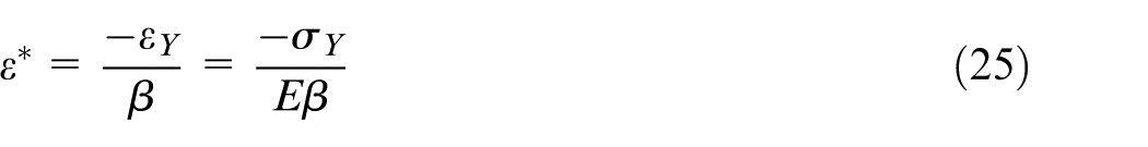
where σ_Y is the yield strength of MS (2.5 × 10⁸ N/m²), and E is the Young’s modulus (2.1 × 10¹¹ N/m²). The restraint force is calculated as follows

F = AE ε^{*}

(26)

where A is the cross-sectional area of the bar and ε* is the inherent strain. The corresponding moment, M, can be calculated as follows

M = \sum F_{1} l_{1} + F_{2} l_{2}

(27)

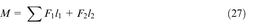
where F₁ and F₂ are the forces at different nodes, and l₁ and l₂ are their corresponding distances from the center of rotation.

Calculation of restraint coefficient

The value of inherent strain depends on the restraint coefficient (β) which further depends on the stiffness of the bar and spring (equation (24)). In general, the inherent strain is determined experimentally by taking a bar and spring of known stiffness and then heating and cooling the bar. However, in this work, an analogy is considered; the weld bead is assumed as the bar as it experiences huge change in temperature during welding. The part of the welded plate adjacent to the weld region is assumed as the spring since this region experiences lesser change in temperature as compared to the weld bead and it acts as a restraint on the weld region. The restraint coefficient is calculated from k (equation (28)) and k* (equation (29))

k = AE / L

(28)

k^{*} = AE / L^{*}

(29)

where k and L are the stiffness and the width of the weld bead, respectively. k* and L* are the stiffness and width the weld plate adjacent to weld bead, respectively. The cross-section area, A, is same for the weld bead as well as of the adjacent plate. Also, the Young’s modulus, E, is same for weld bead and adjacent plate as both are of same material that is MS. Thus, equation (24) can be modified to calculate the restraint coefficient (β) using equations (28) and (29)

β = \frac{L^{*}}{L + L^{*}}

(30)

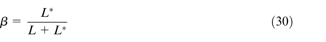
where L is the width of the weld bead whose value is known; however, the value of L* is to be determined. The width of the weld plate (L*) adjacent to the weld bead is considered in such a way that it acts as a spring. In order to determine L*, it is required to analyze the temperature distribution at various points (excluding weld bead region) on the plate during welding.

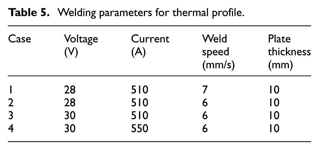
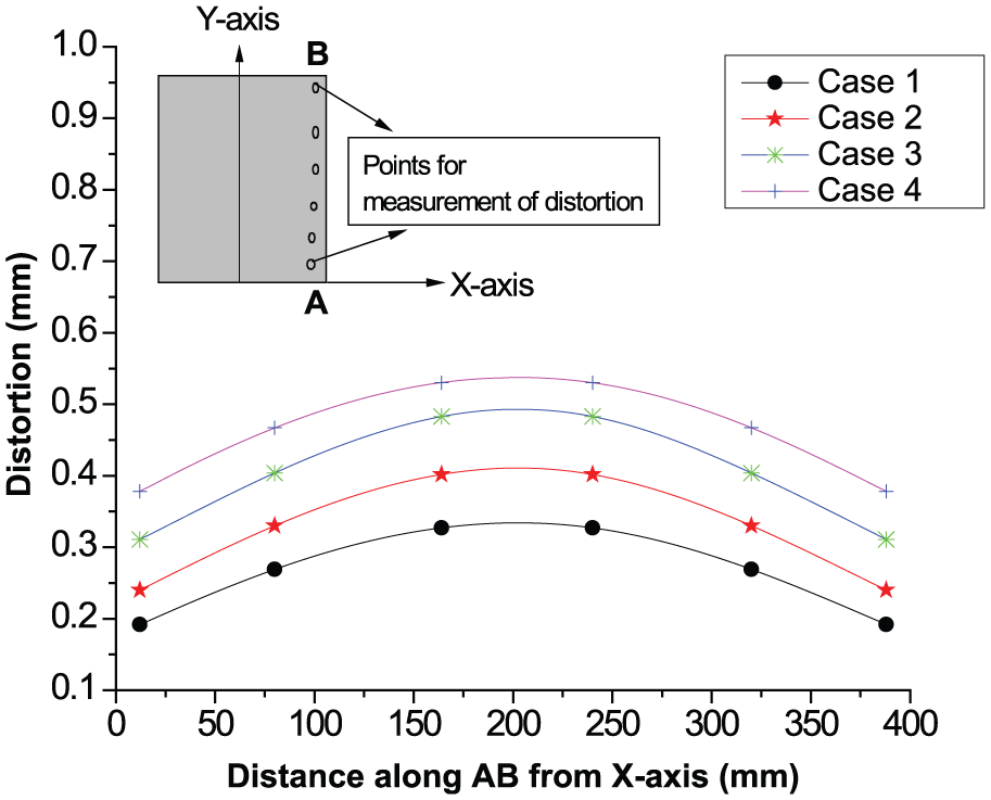
Nonlinear FE transient thermal analysis is performed using surface heat source model of Gaussian distribution to compute the temperature distribution. Figure 8 shows the peak temperatures at different locations on the plate from the weld line considering different cases (Table 5) by changing welding parameters. From Figure 8, it is observed that as the welding parameters such as current and voltage are increased, the peak temperature is more. Increasing welding speed, peak temperature decreases and vice versa. Similarly, the peak temperature decreases for thicker plate and vice versa.

Figure 8.

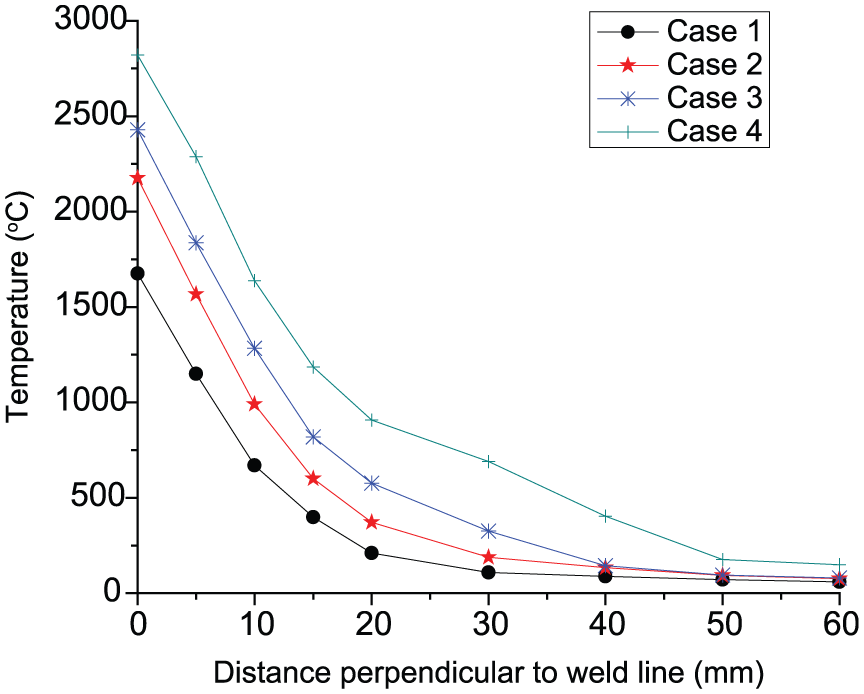
Peak temperatures at different distances from the weld line at different welding parameters (Table 5).

Table 5.

Welding parameters for thermal profile.

Case	Voltage (V)	Current (A)	Weld speed (mm/s)	Plate thickness (mm)
1	28	510	7	10
2	28	510	6	10
3	30	510	6	10
4	30	550	6	10

Here, the width of the plate (L*) is considered as the spring length where peak temperature reaches beyond 100 °C. The spring length is around 50 mm in this study which can be observed in Figure 8. This length varies by changing welding parameters as shown in Figure 8. The restraint coefficient can be calculated using equation (30) with the known value of L and L*. The force and moment at each node are calculated using equations (26) and (27), respectively, and their value summed up at all the nodes in weld bead region. Furthermore, this total value of force and moment is distributed uniformly among the nodes along the line AB (Figure 9) to simulate the distortion in the welded plate considering elastic FE analysis. The distance from the center of the weld line to the line AB is the spring length which was determined from Figure 8. It can be observed from the trial and error experiments that if we consider the spring length as the distance from weld center line to the line where the temperature raises approximately 100 °C provides the best result. It can be seen that the longitudinal shrinkage is very small compared to the transverse shrinkage as shown in Figures 10 –12 and which have a very small effect on welding distortion. Therefore, in this work, for the simplification of the proposed method, the longitudinal shrinkage has been neglected which further reduces the complexity of the model.

Figure 9.

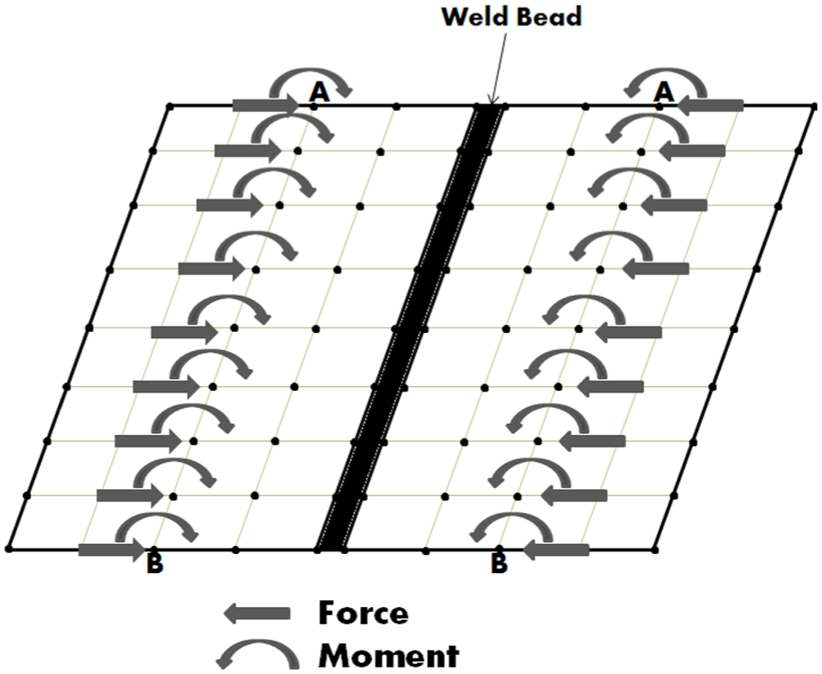
Equivalent mechanical loading.

Figure 10.

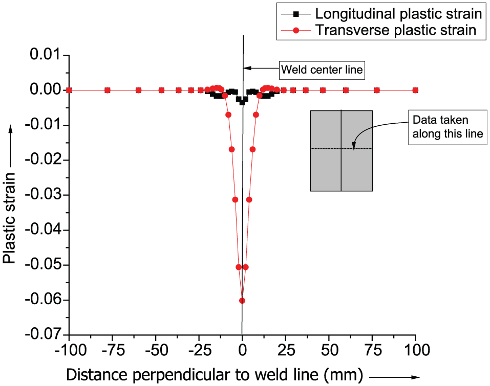
Strain distribution perpendicular to the center of weld line.

Figure 11.

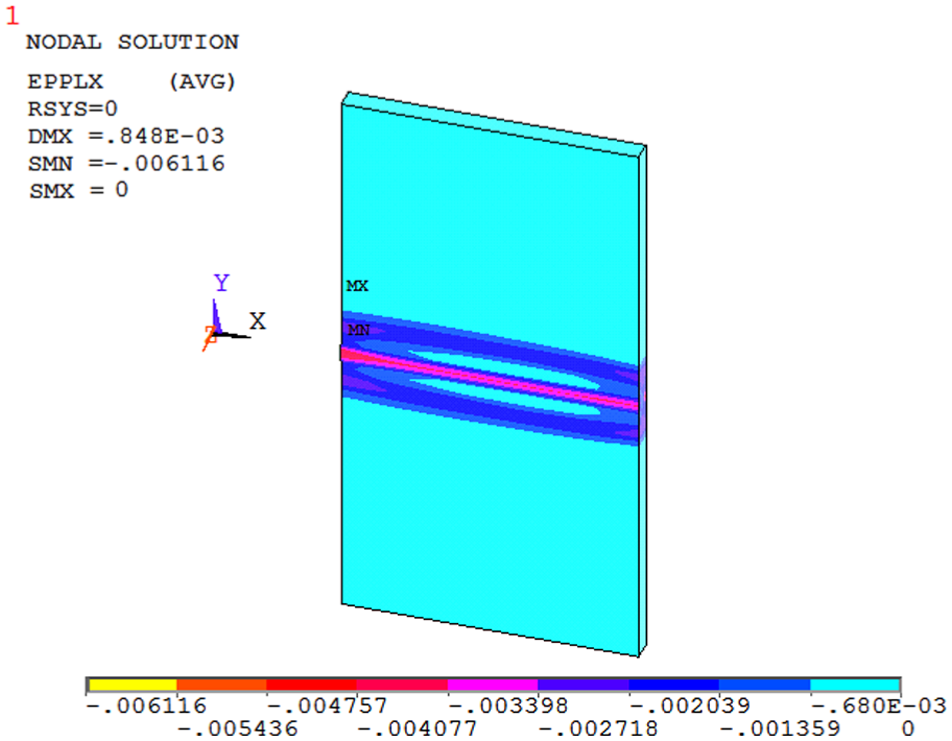
Longitudinal plastic strain distribution contour.

Figure 12.

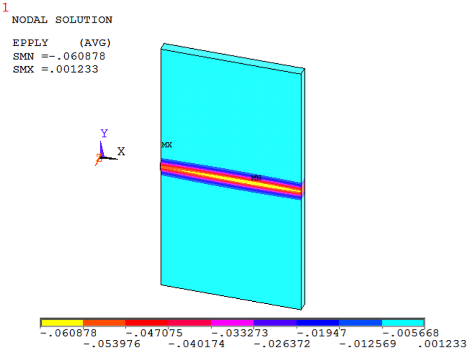
Transverse plastic strain distribution contour.

From Figures 10 –12, it can be observed that the longitudinal strain is very less in comparison with transverse one.

Distortion of butt and fillet welded plates

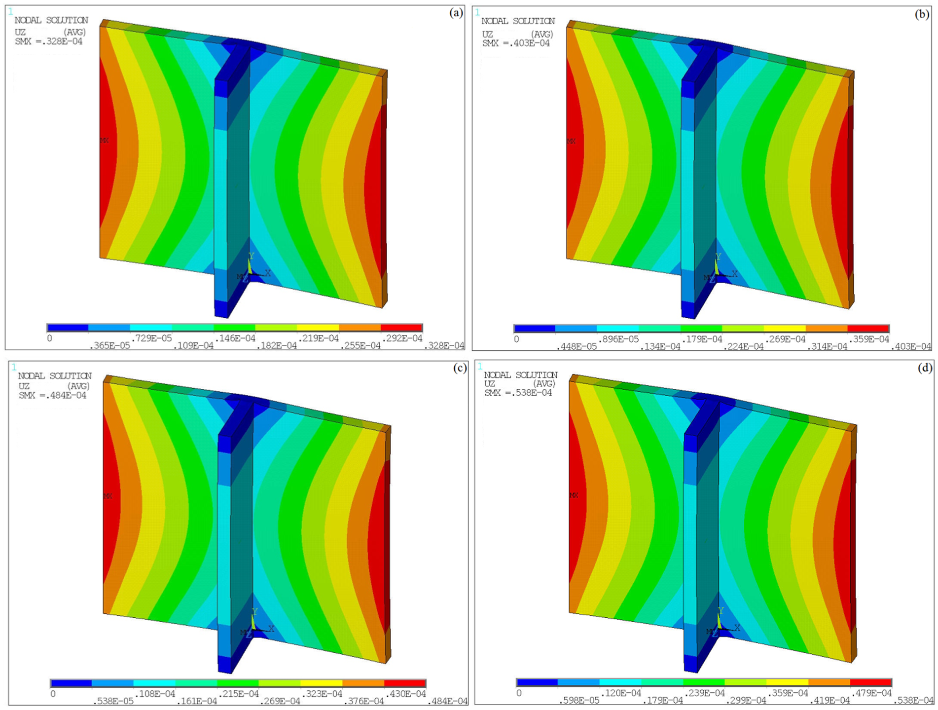
Figure 13(a)–(d) shows the distortion patterns obtained using equivalent loading technique in butt welded plates for different welding parameters as in Table 5.

Figure 13.

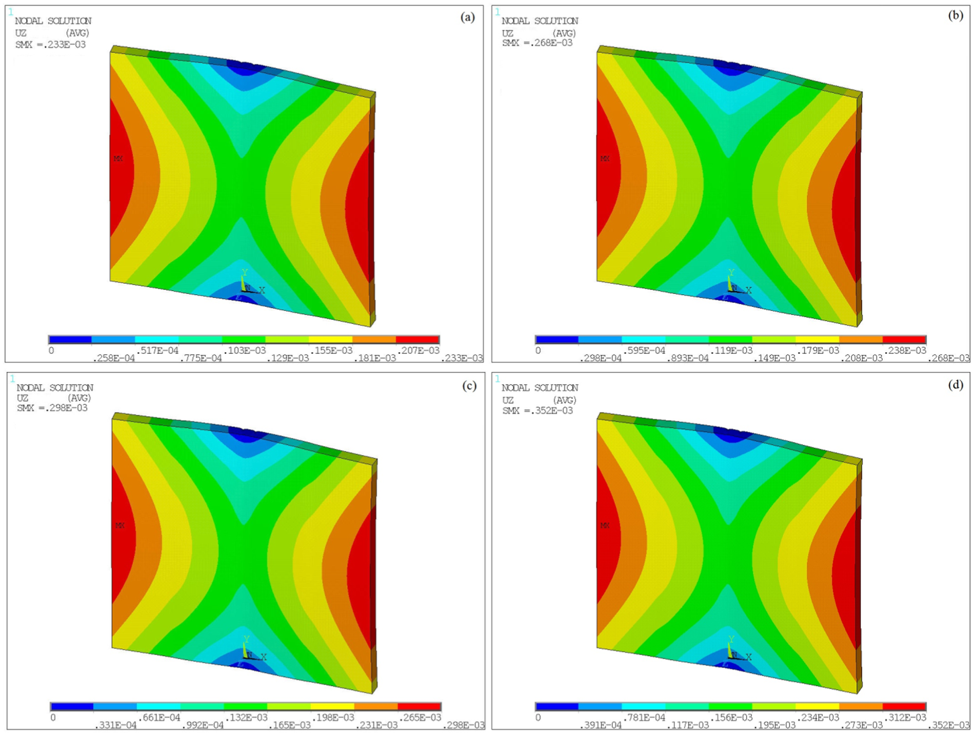
Distortion pattern for butt welded plate for four different cases: (a) Case 1, (b) Case 2, (c) Case 3, and (d) Case 4.

The variation in distortion pattern for change in parameters such as welding current, voltage, speed, and thickness of the weld plates can be observed from these figures. Figure 14 shows the comparison of distortions along the line AB (parallel to Y-axis and close to edge of the plate) considering different cases (Table 5) by changing welding parameters. From Figure 14, it is observed that as the welding parameters such as current and voltage are increased, the distortion is more. Increasing the welding speed decreases the value of distortion and vice versa. Similarly, the distortion decreases for thicker plate and vice versa.

Figure 14.

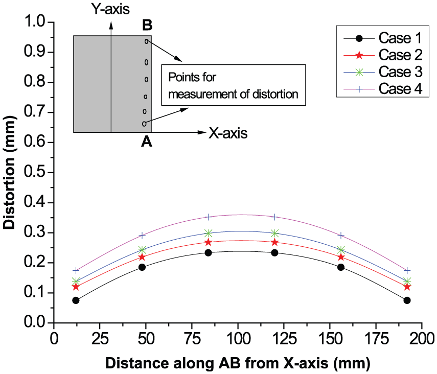
Comparison of distortions along the line AB (parallel to Y-axis and close to edge of the plate) in butt welded plates considering different cases (Table 5).

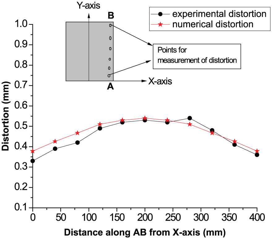
Figure 15 shows the experimental and numerical distortions for a 12-mm-thick square butt welded plate along the line AB (parallel to Y-axis and close to edge of the plate). The welding parameters are given in Table 6. From Figure 15, it is observed that the both distortion patterns match well with a variation of 7%–10% considering maximum distortion value.

Figure 15.

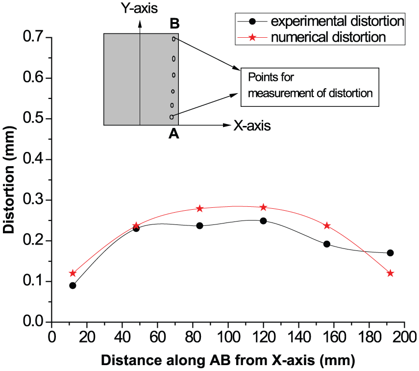
Comparison of numerical and experimental distortion along the line AB (parallel to Y-axis and close to edge of the plate) for 12-mm-thick plate.

Table 6.

Welding parameters for butt welding.

Plate thickness (mm)	Welding parameters
	Current (A)	Voltage (V)	Speed (mm/s)
10	530	28	6

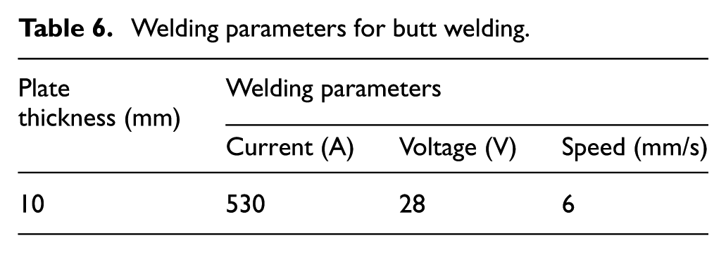
Figure 16(a)–(d) shows the distortion patterns obtained using equivalent loading technique in fillet welded plates for different welding parameters as shown in Table 5. The dimensions of the base plate and web are 400 × 400 × 10 mm and 100 × 400 × 10 mm, respectively. The variation in distortion pattern for change in parameters such as welding current, voltage, speed, and thickness of the weld plates can be observed from these figures. Figure 17 shows the comparison of distortions along the line AB (parallel to Y-axis and close to edge of the plate) in fillet welded plates considering different cases (Table 5) by changing welding parameters. From Figure 17, it is observed that as the welding parameters such as current and voltage are increased, the distortion is more. Increasing the welding speed decreases the value of distortion and vice versa. Similarly, the distortion decreases for thicker plate and vice versa.

Figure 16.

Distortion pattern for fillet welded plate for four different cases: (a) Case 1, (b) Case 2, (c) Case 3, and (d) Case 4.

Figure 17.

Comparison of distortions along the line AB (parallel to Y-axis and close to edge of the plate) in fillet welded plates considering different cases (Table 5).

Figure 18 shows the experimental and numerical distortions for a 10-mm-thick fillet welded plate along the line AB (parallel to Y-axis and close to edge of the plate). The welding parameters are given in Table 5. From Figure 18, it is observed that the both distortion patterns match well with a variation of 5%–9% considering maximum distortion value.

Figure 18.

Comparison of numerical and experimental distortion along the line AB (parallel to Y-axis and close to edge of the plate) for 10-mm-thick fillet welded plate.

Predicted distortion pattern shows a good agreement with the experimental results which proves the reliability of the proposed technique. The time consumed for this analysis is just about 30–40 s. Thus, this technique is efficient and very less time-consuming than the FE thermo-mechanical analysis. Therefore, equivalent loading technique can be used to predict the distortion in a large welded structure.

Large welded structure

The problem of distortion during fabrication process leads to dimensional inaccuracies and misalignments of structural members, which may require corrective tasks or rework if tolerance limit is exceeded. This, in turn, lengthens the production cycle leading to increase in the cost of production. Hence, the problem of distortion and residual stresses are always of great concern in shipbuilding industries. Thus, it is required to assess the extent of possible distortion and residual stresses that may form during fabrication.

Figure 19 shows the large welded plate (2000 × 1400 × 5 mm) with three longitudinal stiffeners (40 × 40 × 6 mm) and two transverse stiffeners (75 × 50 × 6 mm). The end nodes at left and right side lugs are constrained with zero degree of freedom (DOF).

Figure 19.

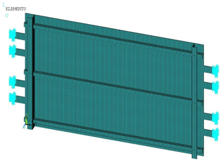
Boundary conditions.

The equivalent loading technique is used to predict the distortion in this large structure. The loads are first applied on the longitudinal stiffeners and solved, after the solution PSTRES, ON is used and then the loads are applied on the transverse stiffeners and then solved to get the final solution. The result is shown in Figure 20. The FE simulation was carried out in a PC having configuration as Intel^® Core^™ i5 CPU, M460@2.53 GHz, 4 GB RAM with Windows 7 operating system. The time taken for this analysis or a large structure with plate dimension of 2000 mm × 1000 mm × 5 mm using combined equivalent loading technique and FE elastic analysis is around 2 min.

Figure 20.

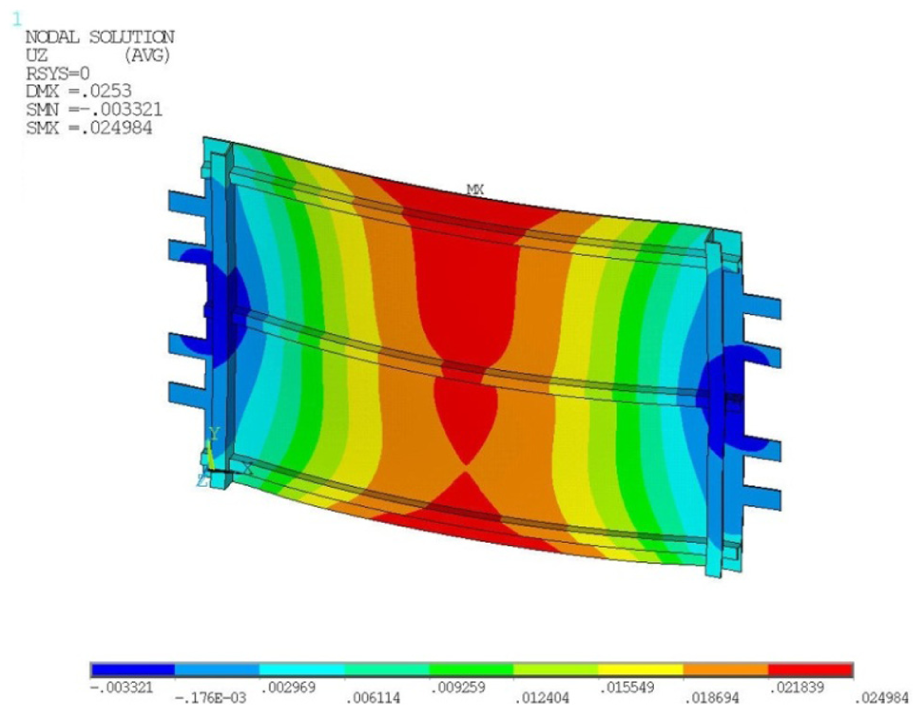
Deformation of a large welded plate.

Table 7 shows the comparison of analysis time between equivalent load technique and conventional technique. It has seen that the structural analysis time is very much less while the equivalent load technique is used, hence saves a lot of time as well as resources.

Table 7.

Comparison of analysis time.

Analysis procedure	Time for thermal analysis (h)	Time for structural analysis
APDL	1.5	3 h
APDL + equivalent load technique	1.5	40 s

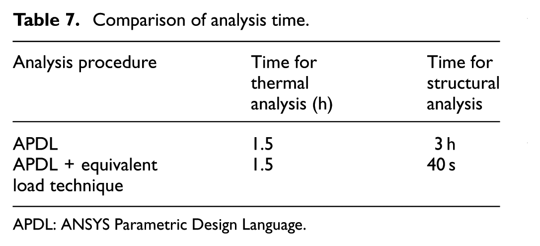
APDL: ANSYS Parametric Design Language.

Conclusion

The following conclusions are drawn from the present investigations.

In the equivalent loading technique, the bar spring analogy is successfully implemented.

The results obtained from the equivalent loading technique are compared with the experimental results and are found to be in reasonable agreement with an error of around 6%–10%. Hence, the technique is proved to be efficient.

The elastic FE analysis using equivalent loading technique involves very less computational time as compared to the 3D FE nonlinear elasto-plastic thermo-mechanical analysis.

Thus, the equivalent loading technique is very useful to predict the distortion in a large welded structure where the simulation time is tremendously greater due to numerous welding passes and sequences.

This method can be effectively used to predict the weld-induced distortion of very large structure with a computation time almost equal to the time required for transient thermal analysis of a small weld structure only.

Although the equivalent loading technique was applied here for the submerged arc welding, it can be noted that similar studies can be possible in all types of fusion welding processes wherever the conventional way of prediction fails to provide any solution quickly.

Footnotes

Declaration of conflicting interests

The author(s) declared no potential conflicts of interest with respect to the research, authorship, and/or publication of this article.

Funding

The author(s) received no financial support for the research, authorship, and/or publication of this article.

References

Kou

. Welding Metallurgy. Wiley-Interscience. 2nd ed. ISBN: 978-0-471-43491-7

Rosenthal

The theory of moving source of heat and its application to metal treatments. Trans ASME 1946; 68: 849–866.

Goldak

Bibby

Moore

et al . Computer modeling of heat flow in welds. Metall Trans B 1986; 17: 587–600.

Watanabe

Satoh

Effect of welding conditions on the shrinkage and distortion in welded structures. Weld J 1961; 40(8): 377–384.

Ueda

Yamakawa

Analysis of thermal elastic-plastic stress and strain during welding by finite element method. Trans Japan Weld Soc 1971; 2: 90–100.

Hibbitt

Marcal

PV.

Numerical thermo-mechanical model for the welding and subsequent loading of a fabricated structure. Comput Struct 1973; 3: 1145–1174.

Rybicki

Schmueser

Stonesifer

et al . A finite-element model for residual stresses and deflections in girth-butt welded pipes. J Press Vess: T ASME 1978; 100(3): 256–262.

Radaj

Heat effects of welding: temperature field residual stress distortion. Springer-Verlag, 1992. ISBN 978-3-642-48640-1.

Luo

Description of inherent strain and its application to prediction of welding deformation and residual stress under multi-pass welding. Doctoral Thesis, Osaka University, Suita, Japan, 1997.

10.

Hong

Tsai

Dong

Assessment of numerical procedures for residual stress analysis of multipass weld. Weld J 1998; 77: 372s–382s.

11.

Dong

Residual stress analyses of a multi-pass girth weld: 3-D special shell versus axisymmetric models. J Press Vess: T ASME 2001; 123: 207–213.

12.

Lindgren

L-E.

Numerical modeling of welding. Comput Method Appl M 2006; 195: 6710–6736.

13.

Tekriwal

Mazumdar

Finite element analysis of three dimensional heat transfer in gas manual arc welding. Weld J 1988; 56: 150–156.

14.

Bonifaz

Finite element analysis of heat flow in single-pass arc welds. Weld J 2000; 79: 121–125.

15.

Friedman

Thermo mechanical analysis of the welding process using the finite element method. Trans ASME 1975; 97: 206–213.

16.

Brown

Song

Implication of three-dimensional numerical simulation of welding of large structures. Weld J 1992; 71: 55–62.

17.

Michaleris

Debiccari

Prediction of welding distortion. Weld J 1997; 76: 172–180.

18.

Mandal

Sundar

Analysis of welding shrinkage. Weld J 1997; 76: 233–238.

19.

Puchaicela

Control of distortion of welded steel structures. Weld J 1998; 77: 49–52.

20.

Biswas

Mahapatra

Mandal

NR.

Numerical and experimental study on prediction of thermal history and residual deformation of double-sided fillet welding. Proc IMechE, Part B: J Engineering Manufacture 2009; 224: 125–134.

21.

Biswas

Mandal

NR.

Thermomechanical finite element analysis and experimental investigation of single-pass single-sided submerged arc welding of C-Mn steel plates. Proc IMechE, Part B: J Engineering Manufacture 2009; 224: 627–639.

22.

Narang

Mahapatra

Jha

et al . Modelling and predicting the effects of submerged arc weldment process parameters on weldment characteristics and shape profiles. Proc IMechE, Part B: J Engineering Manufacture 2012; 226(7): 1230–1240.

23.

Kumar

Batish

Bhattacharya

et al . Effect of process parameters on microhardness and microstructure of heat affected zone in submerged arc welding. Proc IMechE, Part B: J Engineering Manufacture 2010; 225: 711–721.

24.

Lafdani

K-MH

Zahrani

Galloway

A-M.

Optimization study of weld geometry in the tandem submerged arc welding process. Proc IMechE, Part B: J Engineering Manufacture 2015; 229: 1068–1077.

25.

Tsai

Kim

Jaeger

et al . Welding distortion of a thin plate panel structure. Weld J 1999; 78: 156s–165s.

26.

Tsai

Park

Cheng

Design analysis for welding of heavy W shapes. Weld J 2001; 80: 35–41.

27.

Cho

D-W

Kiran

D-V

Song

W-H

et al . Molten pool behavior in the tandem submerged arc welding process. J Mater Process Tech 2014; 214: 2233–2247.

28.

Aucott

Wen

Dong

The role of Ti carbonitride precipitates on fusion zone strength-toughness in submerged arc welded linepipe joints. Mat Sci Eng A: Struct 2015; 622: 194–203.

29.

Paniagua-Mercadoa

A-M

Lopez-Hirataa

V-M

Dorantes-Rosalesa

H-J

et al . Effect of TiO2-containing fluxes on the mechanical properties and microstructure in submerged-arc weld steels. Mater Charact 2009; 60: 36–39.

30.

Shen

Oguocha

INA

Yannacopoulos

Effect of heat input on weld bead geometry of submerged arc welded ASTM A709 Grade 50 steel joints. J Mater Process Tech 2012; 212: 286–294.

31.

Kiran

Basu

Influence of process variables on weld bead quality in two wire tandem submerged arc welding of HSLA steel. J Mater Process Tech 2012; 212: 2041–2050.

32.

Lan

Qiu

Zhao

et al . Analysis of microstructural variation and mechanical behaviors in submerged arc welded joint of high strength low carbon bainitic steel. Mat Sci Eng A: Struct 2012; 558: 592–601.

33.

Luo

Dong

et al . Microstructure of 2205 duplex stainless steel joint in submerged arc welding by post weld heat treatment. J Manuf Process 2014; 16: 144–148.

34.

Jang

Kim

Kam

The effect of root opening on mechanical properties, deformation and residual stress of weldments. Weld J 2001; 80: 80–89.

35.

Hong

Tsai

Dong

. Assessment of numerical procedures for residual stress analysis of multipass weld. Weld J 1998; 77: 372s–382s.

36.

Cho

Lee

Moon

et al . Investigation of residual stress and post weld heat treatment of multi-pass welds by finite element method and experiments. J Mater Process Tech 2004; 156: 1690–1695.

37.

Mahapatra

Datta

Pradhan

et al . Three-dimensional finite element analysis to predict the effects of SAW process parameters on temperature distribution and angular distortions in single-pass butt joints with top and bottom reinforcements. Int J Pres Ves Pip 2006; 83: 721–729.

38.

Souloumiac

Boitout

Bergheau

JM.

A new local global approach for the modelling of welded steel component distortions. London: Maney Publishing, 2002.

39.

Ueda

Kim

Umekuni

Measuring theory of three-dimensional residual stresses using a thinly sliced plate perpendicular to welded line. Trans JWRI 1985; 14(2): 151–157.

40.

Murakawa

Luo

Ueda

Prediction of welding deformation and residual stress by elastic FEM based on inherent strain. J Soc Nav Archit Japan 1997; 180: 739–751 (in Japanese).

41.

Jang

Lee

DE.

Prediction of welding deformations of stiffened panels. Proc IMechE, Part M: J Engineering for the Maritime Environment 2002; 216(2): 133–143.

42.

YS.

Development of thermal distortion analysis method on large shell structure using inherent strain as boundary condition. J Soc Nav Archit Korea 2008; 45(1): 93–100 (in Korean).

43.

Cho

Jang

TW.

Development of welding distortion analysis method using residual strain as boundary condition. Mater Sci Forum 2008; 580–582: 649–654.

44.

Fourier

Theorie analytique de la chaleur (par M. Fourier) Paris: Chez Firmin Didot, père et fils, 1822.

45.

Sabapathy

Wahab

Painter

MJ.

Numerical models of in service welding of gas pipeline. J Mater Process Tech 2001; 118: 14–21.

46.

Biswas

Mandal

NR.

3D FEM and experimental thermo-mechanical analysis of single pass single sided submerged arc welding of C-Mn steel plates. Proc IMechE, Part B: J Engineering Manufacture 2009; 224: 1–13.

47.

Nishikawa

Inherent strains in welding. In: International society of offshore polar engineers conference (ISOPE), Toulon, 23–28 May 2004, pp.126–132. ISBN 1-880653-62–1.

48.

Vega Sáenz

Plazaola

Banfield

et al . Analysis and prediction of welding distortion in complex structures using elastic finite element method. Ship Sci Technol 2012; 6: 35–42.

49.

Nishikawa

Serizawa

Murakawa

. Actual Application of FEM to Analysis of Large Scale Mechanical Problems in Welding. Sci Technol Weld J 2007; 12: 147–152.

50.

Khurram

Shehzad

. FE Simulation of Welding Distortion and Residual Stresses in Butt Joint Using Inherent Strain. Int J Appl Phys Math 2012; 2: 405–408.

Prediction of weld-induced distortion of large structure using equivalent load technique

Abstract

Keywords

Introduction

Experimental investigation

Numerical model

Thermal modeling

Assumptions in thermal model

Formulation of 3D FEA model of heat transfer in arc welding

Boundary conditions

Initial condition 1

Boundary condition 1

Boundary condition 2

Derivation of heat flow matrices

Transient heat flow analysis

Material properties

Thermal history of square butt welding

Equivalent loading technique

Inherent strain

Calculation of restraint coefficient

Distortion of butt and fillet welded plates

Large welded structure

Conclusion

Footnotes

Declaration of conflicting interests

Funding

References