
Abstract
A three-revolute-prismatic-spherical parallel kinematic machine is proposed as an alternative solution for high-speed machining tool due to its high rigidity and high dynamics. Considering the parallel kinematic machine module as a typical compliant parallel mechanism, whose three limb assemblages have bending, extending and torsional deflections, this article proposes a hybrid modeling methodology to establish an analytical stiffness model for the three-revolute-prismatic-spherical device. The developed analytical model is further used to evaluate the stiffness mapping of the three-revolute-prismatic-spherical module over a given work plane which is then validated by experimental tests. The simulations and experiments indicate that the present hybrid methodology can predict the three-revolute-prismatic-spherical parallel kinematic machine’s stiffness in a quick and accurate manner. The solution for eigenvalue problem of the stiffness matrix leads to the stiffness characteristics of the parallel module including eigenstiffnesses and the corresponding eigenscrews as well as the equivalent screw spring constants. Based on the eigenscrew decomposition, the parallel kinematic machine is physically interpreted as a rigid platform suspending by six screw springs. The minimum, maximum and average of the screw spring constants are chosen as indices to assess the three-revolute-prismatic-spherical parallel kinematic machine’s stiffness performance. The distributions of the proposed indices throughout the workspace reveal a strong dependency on the mechanism’s configurations. At the final stage, the effects of some design parameters on system stiffness characteristics are investigated with the purpose of providing useful information for the conceptual design and performance improvement of the parallel kinematic machine.
Keywords
Introduction
High-speed machining (HSM) has been recognized as one of the key manufacturing technologies for high productivity and throughput. However, the definition of HSM is not easy since the actual cutting speed that can be achieved depends on the work material, the type of cutting operation, the cutting tool used and so on. 1 In compliance with modern knowledge, the Institute of Production Engineering and Machine Tools (PTW) at the Darmstadt University of Technology defined high-speed machining as being where conventional cutting speeds of a particular material are exceeded by a factor of 5–10. 2 From the productivity point of view, HSM is not only a technical index but also an economical index, which can achieve higher productivity and throughput. Compared with their counterparts of serial machine tools, parallel kinematic machines (PKMs) with lower mobility have found their promising potentials in HSM due to the merits of simple structure, high rigidity, better accuracy, good reconfigurability and easy controlling. For example, machining an aircraft wing over 30 m long would require a huge gantry five-axis machine tool with tons of weight and large footprint. However, a much more compact device with comparable machining accuracy can be achieved by using a parallel arrangement. This has been fully exemplified by the commercial success of the Sprint Z3 Head and the Tricept robots applied in aeronautical and automobile industries for HSM tasks.3–5 Other propositions of applying PKMs for HSM can also be traced in recent publications.6–9
Inspired by the successful application of Sprint Z3 Head, a similar three-degree-of-freedom (3-DOF) PKM module was proposed with one translational and two rotational capabilities, whose topological structure is a three-revolute-prismatic-spherical (3-RPS) parallel mechanism. 10 Added by an x–y motion, this proposed design can be used as a multiple-axis spindle head to form a hybrid five-axis HSM unit. When designed for HSM applications, such a kind of PKM module needs to meet the requirements of high rigidity and high positioning accuracy, which makes stiffness become the most overwhelming concern in the design stage. The evaluation of a PKM’s stiffness performance involves two kernel issues, that is, stiffness modeling and evaluation indices.
For the first issue, the substantial work is how to establish a mathematical model to reflect the platform’s ability of resisting deflections subject to external loads. And such an ability of a PKM can be generally described by a 6 × 6 stiffness matrix, which relates the vector of compliant deformations of the PKM to an external static wrench applied at the end-effector. Unlike the hexapod parallel manipulator, whose stiffness matrix can be straightforwardly derived by considering the compliances of each component, the derivation of the overall stiffness matrices for lower mobility parallel manipulators, such as a 3-RPS PKM module, is quite difficult due to their kinematic and complex structural features. 11
Numerous efforts can be traced toward the stiffness modeling of lower mobility parallel manipulators in the past decades. Among all these efforts, the finite element method (FEM),12,13 the matrix structure method (MSM),14,15 the virtual joint method (VJM)16–18 and the screw-based method (SBM)19–22 are the most commonly used approaches. For example, Huang et al. 14 proposed a stiffness model for a tripod-based PKM by decomposing the overall system into two separate substructures and formulating the stiffness expressions of each substructure with virtual work principle. A similar model of the 3-DOF CaPaMan parallel manipulator was established by Ceccarelli and Carbone, 18 which considered the kinematic and static features of three legs in view of the motions of each joint and link. Considering the compliances of actuations and constraints, Li and Xu 20 proposed an intuitive method based on an overall Jacobian to formulate the stiffness matrix of a three-prismatic–universal–universal (3-PUU) translational PKM. And the overall stiffness matrix of the lower mobility parallel manipulator could be derived intuitively. Following the same track, Huang et al. 21 proposed a stiffness modeling approach for lower mobility parallel manipulators by using the generalized Jacobian. Dai and Ding 22 proposed a comprehensive analytical compliance model for a three-legged rigidly connected platform device. By solving the eigenvalue problem, the eigencompliances and eigentwists of the flexible parallel mechanism were obtained and the effects of design parameters on compliance property were outlined.
As evidenced by the literatures, the challenge of stiffness modeling is how the proposed mathematical model can predict the stiffness performance over the entire workspace precisely and quickly. This is of great importance in that in most circumstances a PKM’s stiffness is strongly dependent on the manipulator’s configurations, which makes an FE model with large DOFs unacceptable due to high computational cost. On the contrary, an analytical stiffness model may be computationally efficient but lack accuracy when used to predict the PKM’s stiffness. Accordingly, it might be an applaudable choice to develop a hybrid stiffness model that combines the benefits of accuracy of the FEM and concision of the analytical method. Hence, such a kind of hybrid model can be used to predict the stiffness characteristics of a PKM throughout its entire workspace in a quick and accurate manner. This can be useful to evaluate whether the design is satisfied with the stiffness requirements or even further to perform an optimal design with the stiffness considered especially in the design stage. In addition, it is necessary to investigate the stiffness behavior of a PKM at specified configurations to have an in-depth understanding of its stiffness behavior.
As to the second issue in the stiffness design process of a PKM, the fundamental consideration is to provide a proper or suitable index to evaluate its stiffness performance. The authors’ review of previous investigations shows that several performance indices have been proposed for the stiffness evaluation of PKMs. The simplest one is to use stiffness factors, that is, the entries of the stiffness matrix. This, however, is only applicable to evaluate a PKM with diagonal stiffness matrix.14,23 Additionally, the trace and/or determinant of a stiffness matrix has been adopted to assess the stiffness of parallel manipulators.18,24 However, a high value of the determinant or trace does not definitely mean good stiffness performance of a PKM. For example, when a manipulator possesses very low rigidity in one direction but with very high stiffness in other directions, the determinant or trace may be very high but the low stiffness direction may prohibit its application as machining tools. Furthermore, the condition number of the stiffness matrix has been introduced, and then a global stiffness index defined as the inverse of the condition number of the stiffness matrix integrated over the reachable workspace and divided by the workspace volume is presented to assess the stiffness of a 3-DOF spherical parallel manipulator. 25 The proposition of condition number of a stiffness matrix can indicate the ill-conditioning of a PKM but cannot provide direct information on stiffness values.
Besides the aforementioned indices, there is another way to evaluate the stiffness performance of a PKM, that is, to use the eigenvalue of the stiffness matrix. It has been verified that the stiffness is bounded by the minimum and maximum eigenvalues of the stiffness matrix. 26 If a PKM is designed for machining tool application, the minimum stiffness throughout the workspace should be over a threshold to ensure the machining accuracy. From this point of view, it is reasonable to adopt the minimum and maximum eigenvalues of stiffness matrix as indices to evaluate the stiffness performance for the proposed 3-RPS PKM design.
Considering the proposed design as a compliant parallel mechanism where the three RPS limbs are equivalent to three sets of springs, which have bending, extending and torsional deflections, this article presents a comprehensive hybrid stiffness model for the 3-RPS PKM module and an in-depth investigation of the system stiffness properties. The analysis is then extended to the effects of design parameters on the system rigidity in order to provide a designer with useful information in the conceptual design stage.
Kinematic description
A computer-aided design (CAD) model for the 3-RPS PKM is shown in Figure 1.
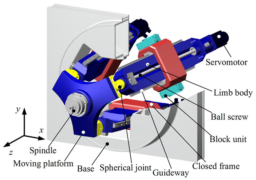
Structure of the 3-RPS design.
As shown in Figure 1, the 3-RPS PKM module consists of a moving platform, a fixed base and three identical kinematic limbs. Each limb connects the fixed base to the moving platform by a revolute (R) joint which is followed by a prismatic (P) joint and a spherical (S) joint in sequence, where the P joint is driven by a lead-screw linear actuator. An electrical spindle is mounted on the platform to implement high-speed milling. Independently driven by three servomotors, one translation along the z-axis and two rotations about the x-axes and y-axes can be achieved. The detailed descriptions of mechanical features of the 3-RPS design were addressed in our previous work. 27
For the purpose of analysis, a schematic diagram of the 3-RPS PKM is depicted in Figure 2. Herein, Ai and Bi (i = 1–3) are the centers of spherical and revolute joints, respectively; Ci denotes the rear end of the limb; ΔA1A2A3 and ΔB1B2B3 are assumed to be equilateral.
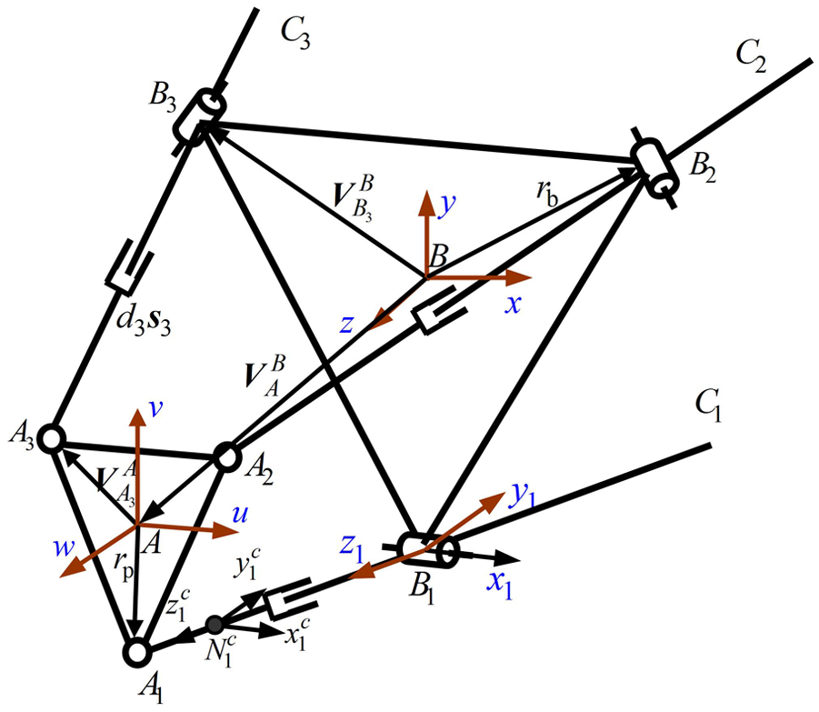
Schematic diagram of the 3-RPS PKM in Figure 1.
In order to work out a suitable formulation, Cartesian coordinate systems are set as follows. The reference coordinate system B-xyz is attached at the center point B of the fixed base, with the x-axis parallel to B2B3 and the z-axis normal to ΔB1B2B3; the body-fixed coordinate system A-uvw is placed at the center point A of the moving platform, with the u-axis parallel to A2A3 and w normal to ΔA1A2A3; the limb reference frame Bi-xiyizi is established at the center point Bi of the ith revolute joint, with xi and zi coincident with the axes of revolute joints and limbs, respectively; the centroid reference frame
Assume the transformation matrix
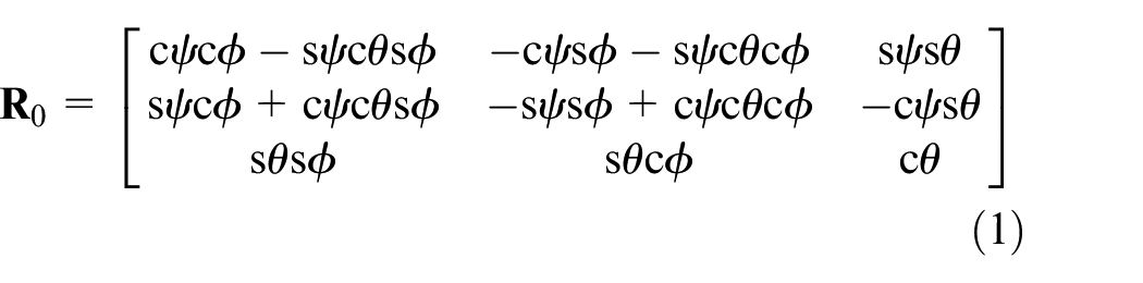
where “s” and “c” denote “sin” and “cos” functions, respectively; ψ, θ and ϕ are the Euler angles in terms of precession, nutation and rotation, respectively.
Vectors of points A and Bi measured in the B-xyz frame are defined as
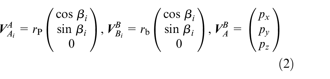
where rp and rb are the radii of the moving platform and the fixed base, respectively;
Supposing di denotes the distance between Ai and Bi and

Considering the constrains of revolute joint and taking ψ, θ and pz as independent coordinates, one can obtain the following
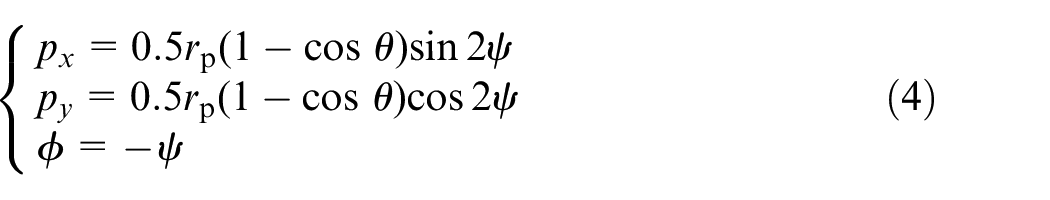
Equation (4) represents the parasitic motion of the 3-RPS mechanism. Thus, the inverse position analysis can be conducted by using the following expressions

Further derivation can give the transformation of the frame Bi-xiyizi with respect to the frame B-xyz as

where
Stiffness modeling
This section aims to formulate the stiffness expression of an individual limb as well as that of the PKM system by considering all significant compliances simultaneously. The considered compliances include bending, extension and torsion deflections of the limb body and the deflections of the prismatic, spherical and the revolute joints.
Assumptions
For the convenience of analytical derivation, the following hypotheses and approximations are made:
The fixed base and moving platform are treated as rigid bodies due to their relatively high rigidities.
The limb body is modeled as a continuous elastic hollowed spatial beam with non-uniform cross sections according to its structural features.
The revolute and spherical joints are simplified into virtual lumped springs with equivalent stiffness at their geometric centers.
The dampings and frictions in all kinematic pairs are neglected although they can be added to the governing equations with further efforts.
Equilibrium equations of an individual RPS limb assembly
Figure 3 shows the mechanical design of an RPS limb in the 3-RPS PKM module.
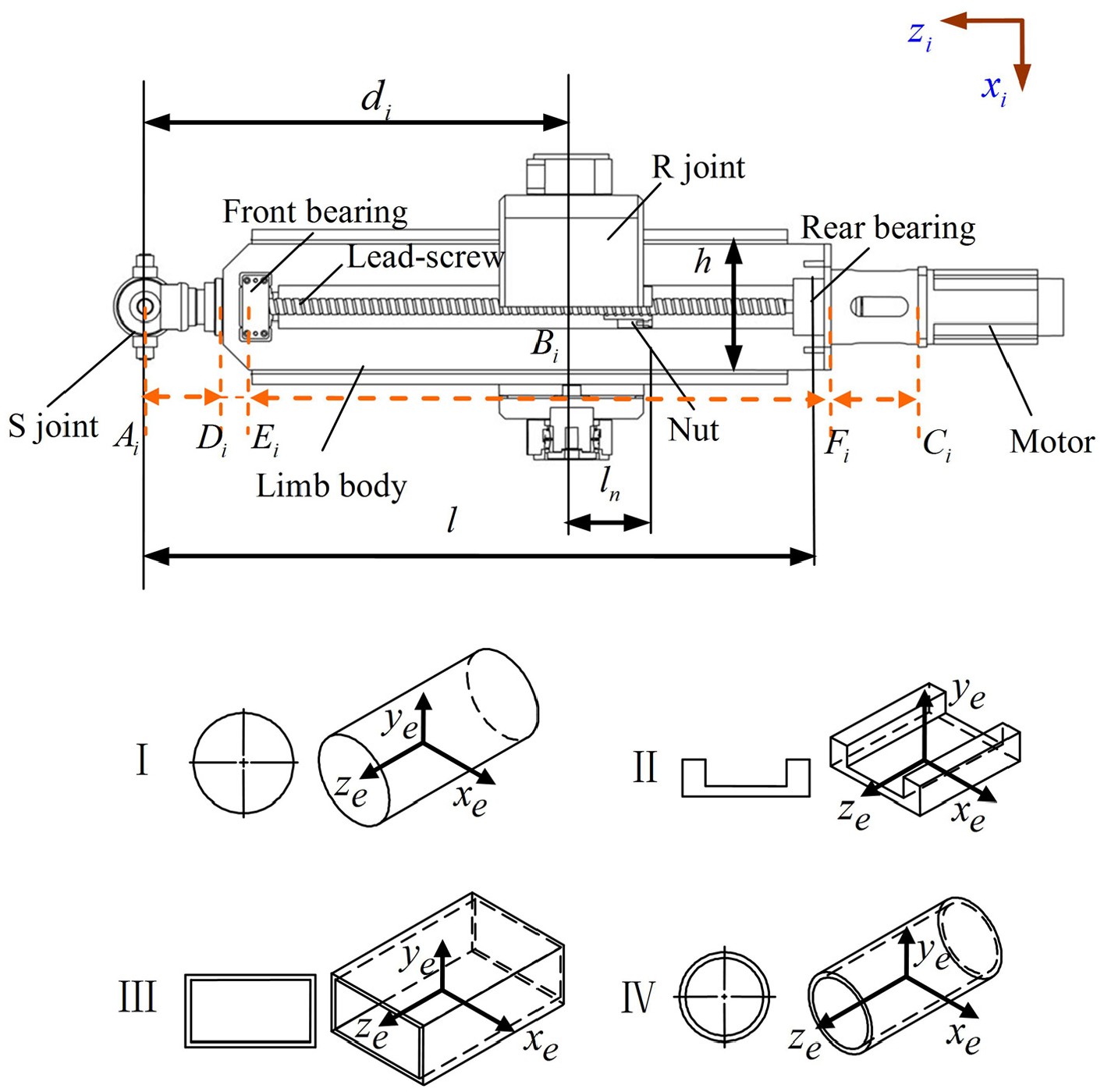
Assembly of an RPS limb.
According to the assembling relationships and structural features of the limb, one can classify all the components in an individual RPS limb into three categories when considering compliance modeling: (1) the limb body, (2) the revolute joint (including the lead-screw assembly) and (3) the spherical joint. Consequently, the compliance of an entire RPS limb can be modeled as a serial combination of the aforementioned three compliant components.
As can be seen from Figure 3, the cross sections of the limb body are non-uniform. To be specific, the cross section of segment AiDi of the limb body is in a cylinder form with gradually changing dimensions. The topological form of the cross section is depicted as I. Accordingly, the cross sections of segments DiEi, EiFi and FiCi are labeled as II, III and IV, respectively. By considering the structural features of the limb body, the limb body is modeled as a spatial beam with non-uniform cross sections. As mentioned above, the revolute and spherical joints are represented as virtual lumped springs with equivalent stiffness at their geometric centers. Thus, the RPS assembly can be modeled as a spatial beam supported by two sets of lumped springs as shown in Figure 4. Herein, ksxi, ksyi and kszi are linear stiffness coefficients of the ith spherical joint; krxi, kryi, krzi and krui, krvi, krwi are linear stiffness coefficients and angular stiffness coefficients of the ith revolute joint in the ith limb assembly, respectively.
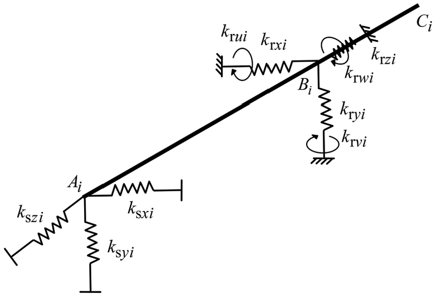
Simplified force diagram of the ith limb.
The following will introduce the computation of compliances of the revolute and spherical joints, with which the stiffness coefficients of ksxi, ksyi, kszi and krxi, kryi, krzi, krui, krvi, krwi can be obtained.
Compliance of revolute joint assembly
As shown in Figure 3, the revolute joint consists of two R joint bearings, a closed frame, two parallel guideway assemblies and a lead-screw assembly containing a front bearing, a rear bearing, a lead screw and a nut. Supposing
The R joint bearing provides constraints in five directions and only allows the rotation about its axis. Hence, the compliance matrix of the R joint bearing
where
Similarly, the compliance matrix of the closed frame
where
The closed frame is installed on the fixed base through the guideway assembly, which can be simplified into a virtual lumped spring with compliance in six directions. Apparently, this virtual lumped spring does not provide constraint to the closed frame along the axial direction of the guideway. Therefore, the compliance of the guideway assembly can be formulated as

where
The lead-screw assembly serially comprises the nut, the lead screw, the front bearing and the rear support bearing, which only provides constraint to the carriage in axial direction. Thus, its compliance can be expressed as

where
where E is the tensile modulus of the lead screw;
Substituting equations (10)–(14) into equation (9), one can formulate the compliance of revolute joint assembly as

The elements in the above equation can be calculated in detail as follows:
Compliance of spherical joint assembly
The spherical joint connects the limb body to the moving platform and can be simplified as a virtual lumped spring with compliance in three orthogonal translational directions. The compliance matrix of a spherical joint can be expressed as

It is worthy to point out that the compliance of a spherical joint is the superposition of the compliances of three revolute joints whose axes are orthogonal to each other and thus varies with joint configurations. The detailed derivation process for the spherical joint stiffness was discussed in Li et al. 10 and will not be addressed here.
FE formulation of limb body
To simplify the formulation, each limb body is discretized into n − 1 elements with Ci, Bi and Ai being nodes of elements.
As a result, a set of equilibrium equations of the ith limb in frame Bi-xiyizi can be formulated with adequate boundary conditions. For convenience, the subscript except the limb body number i (i = 1, 2, 3) is omitted

where
One may define transformation matrices of
The coordinate transformation can be made to express equation (18) in the reference coordinate system B-xyz as


where

Validation of the proposed FE model
In order to verify the accuracy of the above modeling method for the limb body, one individual limb body is taken as an example and its stiffness characteristics are analyzed both with the proposed spatial beam FE model and commercial software ANSYS. To compare this, one end of the limb body (the motor base, Ci) is fixed while a force of 1000 N in the x- and y-directions is applied at the other end (the spherical joint, Ai), respectively. Figure 5(a) and (b) show the deformations of the limb body in the x- and y-directions obtained from ANSYS, respectively. The maximum deflections in the x- and y-directions at the end of the limb body are 0.046 and 0.145 mm while the analytical results from the spatial beam model are 0.047 and 0.141 mm, respectively. The calculation errors are less than 5%. Figure 5(c) and (d) demonstrate the deformations in the x- and y-directions of the limb body along the z-axis obtained from the two methods. It can be found clearly that the results of two models agree very well, indicating that the proposed spatial beam model has a satisfactory accuracy, thus can be used to predict the stiffness characteristics of the limb body.
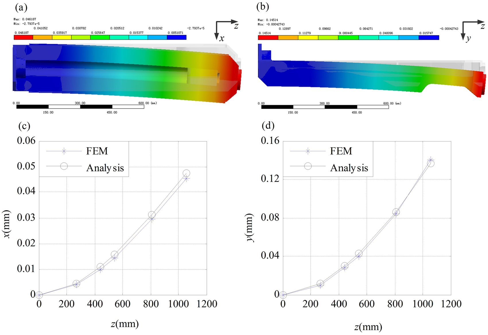
Deformations of an individual limb body: (a) deformation nephogram in x-direction, (b) deformation nephogram in y-direction, (c) deformation in x-direction and (d) deformation in y-direction.
Equilibrium equations of the moving platform
The free body diagram of the moving platform is shown in Figure 6. Herein,

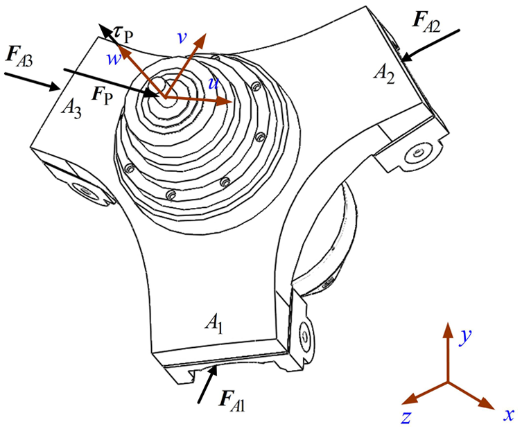
Force diagram of the moving platform.
According to Figure 6, the equilibrium equations of the moving platform can be formulated
Deformation compatibility conditions
As mentioned above, the moving platform connects with the ith limb assembly through a spherical joint, which can be treated as a virtual lumped spring with equivalent stiffness. The displacement relationship between the platform and the limb can be demonstrated as Figure 7, in which AiM and AiL are the interface points associated with the moving platform and RPS limb, respectively.
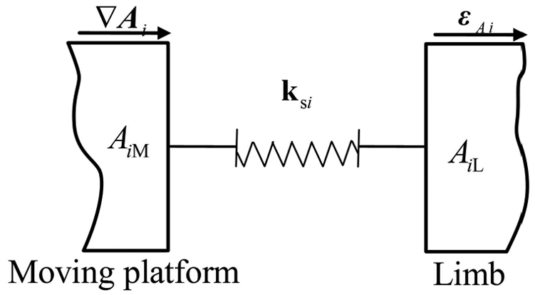
Displacement relationship between the platform and the limb body.
Observing that the elastic motion of moving platform

where
Combining equations (19) and (21), the linear coordinate of node Ai can be expressed as

As a result, the difference between the elastic displacements of AiM and AiL in the limb coordinate system Bi-xiyizi can be derived

Noting that the spherical joint connects the moving platform with the link at Ai, one can express the reaction forces of the spherical joint as

Similarly, the reactions at Bi are

where
Governing equilibrium equations of the system
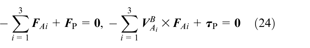
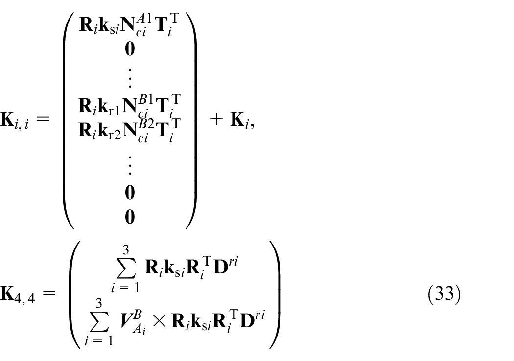
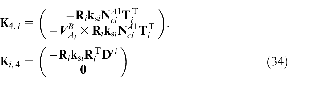
Inserting equations (28) and (29) into equations (20) and (24), one can write the equilibrium equations of the PKM system as

where
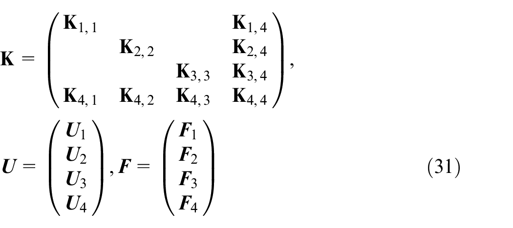
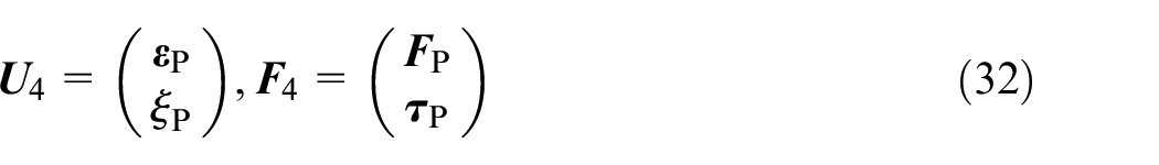
And the global stiffness
Stiffness matrix of the moving platform
In order to evaluate the rigidity of the moving platform, the concept of compliance is adopted, which is mathematically expressed as

where H = 18n + 6 is the dimension of the stiffness matrix and n is the number of discrete nodes on each limb body.
With equation (35), the compliance matrix of the platform can be obtained as the last 6 × 6 block matrix in
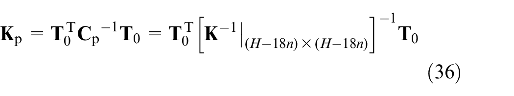
where
Stiffness evaluation of the 3-RPS PKM
The major architecture parameters of a 3-RPS PKM are listed in Table 1. Herein, θmax denotes the maximum rotation angle of the platform about the u- and v-axes; s represents the stroke of the moving platform; l is the length of the limb body as shown in Figure 3; dlead is the diameter of the lead screw; dmin denotes the minimum distance between the spherical joint and revolute joint in limb i. The meaning of the other symbols can be referred to the aforementioned context. These architecture parameters are designed to achieve a compromise between global dexterity and rigidity performance over the entire workspace by using the proposed formulation. According to this rule, the workspace of the design is set with motion ranges θu = ±40°, θv = ±40° and pz = 540–740 mm.
The architecture parameters of a 3-RPS PKM (unit: mm).
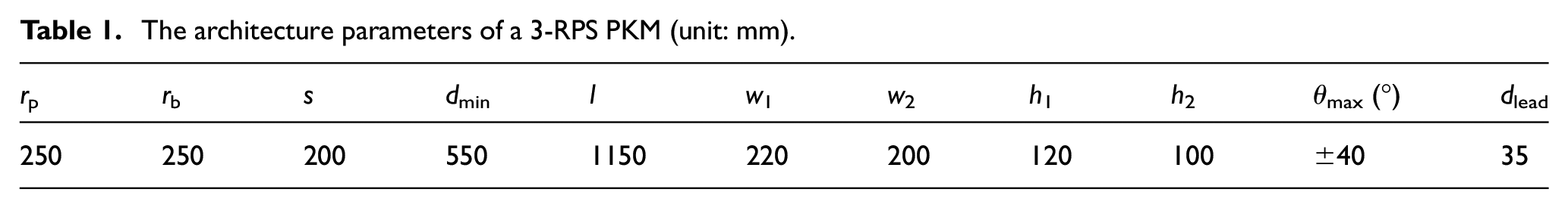
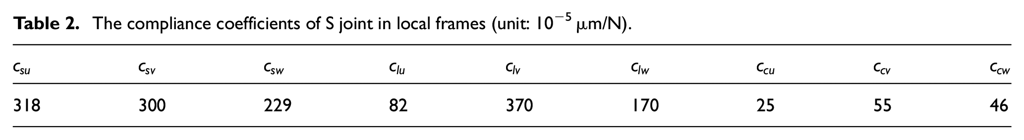
Table 2 gives the compliance coefficients of three perpendicular axes of a spherical joint in its local frame. In addition, the elastic modulus and shear modulus of the limb body and lead screw are assumed as
The compliance coefficients of S joint in local frames (unit: 10−5 µm/N).
Based on the above parameters of the example system, the following simulations can be carried out.
Stiffness distributions over a given work plane and experimental validation
Figure 8 shows distributions of stiffness values along and about the u-, v- and w-axes over the work plane at pz = 560 mm. Herein, k11, k22 and k33 denote linear stiffnesses along the u-, v- and w-axes, respectively; k44, k55 and k66 represent angular stiffnesses about the u-, v- and w-axes, respectively;
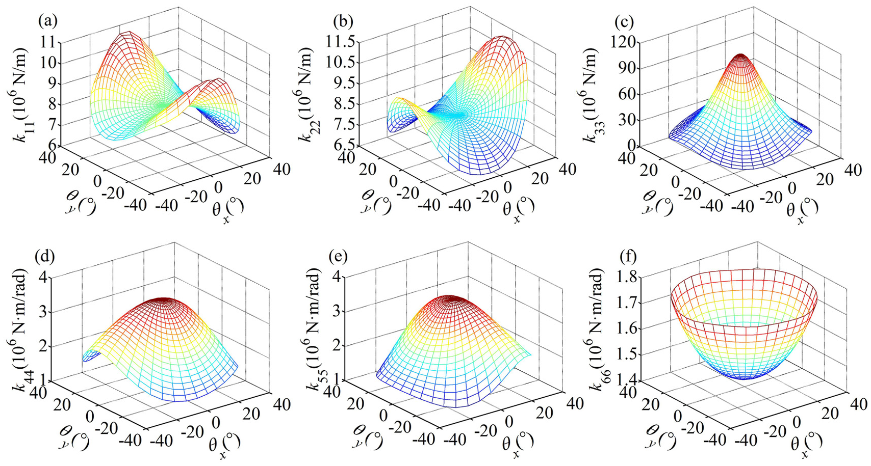
Distributions of stiffnesses when pz = 560 mm: (a) stiffness along the u-axis, (b) stiffness along the v-axis, (c) stiffness along the w-axis, (d) stiffness about the u-axis, (e) stiffness about the v-axis and (f) stiffness about the w-axis.
It is obvious that the stiffness distributions are strongly position-dependent. For instance, the linear stiffness along the u-axis k11 changes from the minimal value 6.15 × 10⁶ N/m to the maximal value 1.06 × 10⁷ N/m, and the linear stiffness along the v-axis k22 changes from 6.74 × 10⁶ to 1.12 × 10⁷ N/m. The linear principle stiffness along the w-axis k33 varies from 1.48 × 10⁷to 1.14 × 10⁸ N/m. By observing Figure 8(a) and (b), one can find that when the moving platform swings about the x-axis, the linear stiffness along the u-axis k11 decreases while that along the v-axis k22 increases. On the contrary, when the moving platform swings about the y-axis, k11 increases while k22 decreases. Interestingly, there is a common point between k11 and k22 in that their distributions are symmetric about the y-axis. Further observations reveal that distributions of the other four stiffnesses are symmetric, that is, 120° symmetric about the z-axis, which is coincident with the structure feature of the PKM that three RPS limb assemblies are distributed 120° symmetrically. It can also be found that the linear stiffness values along the w-axis k33 are comparatively larger than those of k11 and k22 when the two rotation angles are in a small scale; on the contrary, the angular stiffness values about the w-axis k66 are comparatively smaller than those of k44 and k55 when the two rotation angles are in a small scale. This indicates that the proposed PKM possesses a ‘strong’ rigidity along the tool axis but a ‘weak’ one about the tool axis.
In order to verify the accuracy of the proposed stiffness model, a static stiffness experiment is conducted. Figure 9 illustrates stiffness measurement setups of the 3-RPS PKM. A lifting-jack-like mechanism is used to apply external point forces at the end of moving platform; a force indicator is used to show the magnitude of the applied forces; the deflections subject to external forces at five typical collecting points can be measured by micrometers 1–5. Herein, the 1–4 micrometers are used to eliminate the measurement errors caused by the elasticity of the base.
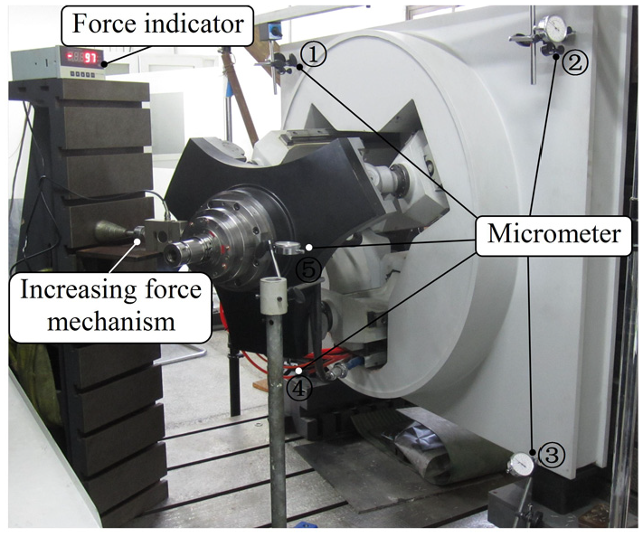
Stiffness measurement setups.
Figure 10 illustrates the comparison between the analytical results and experimental results. Figure 10(a) shows the variations of the linear stiffness along the u-axis k11 with respect to pz. It can be found that both the analytical and the experimental stiffnesses along the u-axis decrease with the increment of pz. To be specific, the analytical stiffness along the u-axis decreases from 8.35 to 6.48 N/µm with the increment of pz while the experimental one decreases from 8.34 to 6.43 N/µm with the increment of pz. Figure 10(b) represents the variations of the linear stiffness along the u-axis k11 with respect to θy when pz = 560 mm, θx = 0°. It is obvious that both the analytical and the experimental stiffnesses along the u-axis increase with the increment of θy. For instance, the analytical stiffness along the u-axis increases from 8.15 to 9.76 N/µm with the increment of θy while the experimental one increases from 7.88 to 10.68 N/um with the increment of θy. Further calculation reveals that all the calculation errors between the analytical simulations and experimental tests are less than 10%. Therefore, it can be concluded that the results of the analytical method and experimental tests agree very well, indicating that the proposed stiffness model has a satisfactory accuracy, thus can be used to predict the stiffness characteristics of the 3-RPS PKM.
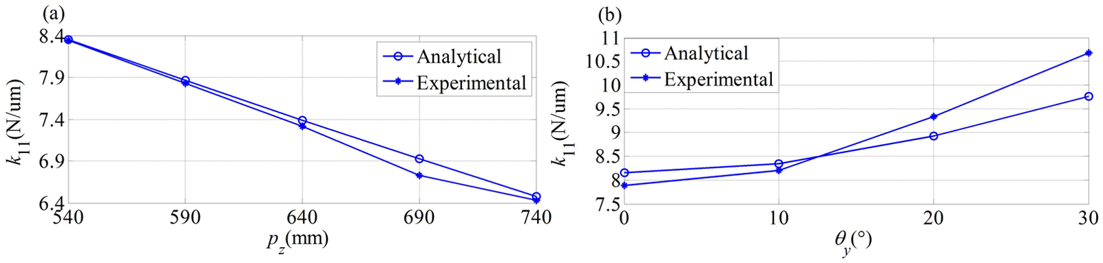
Comparison between analytical results and experimental results: (a) stiffness along the u-axis when θx = θy = 0° and (b) stiffness along the u-axis when pz = 560 mm, θx = 0°.
Stiffness interpretation through eigenscrew decomposition
It can be found from equation (31) that the global stiffness matrix is coupled, which makes it hard to evaluate the rigidity of the moving platform. Therefore, in this subsection, the stiffness behavior of the 3-RPS PKM module is investigated through the eigenscrew decomposition of the stiffness matrix.
The eigenscrew problem formulated in ray coordinates is described as
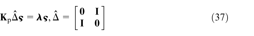
where the eigenvalue
Based on equation (37), the eigenscrew decomposition of the stiffness matrix can be expressed as
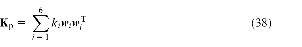
where
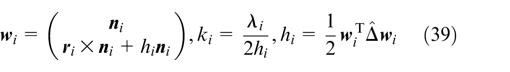
where
Equation (38) indicates that
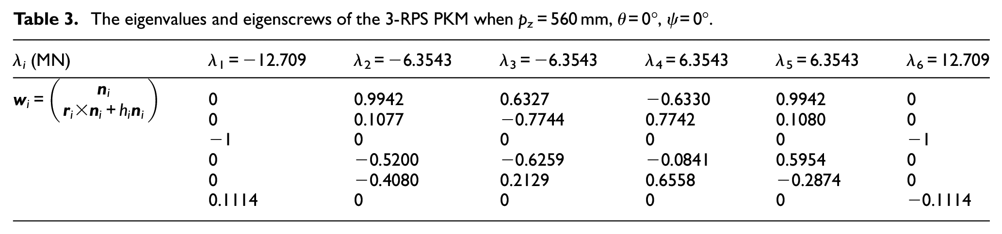
Taking the 3-RPS PKM at a configuration where pz = 560 mm, θ = 0°, ψ = 0° as an example, the eigenvalues and the corresponding eigenscrews of the system can be obtained by solving the eigenvalue problem of equation (37). The results are listed in Table 3. And the physical properties and geometrical entities of the six screw springs can be listed as in Table 4.
The eigenvalues and eigenscrews of the 3-RPS PKM when pz = 560 mm, θ = 0°, ψ = 0°.
The equivalent six screw springs based on eigenscrew decomposition when pz = 560 mm, θ = 0°, ψ = 0°.
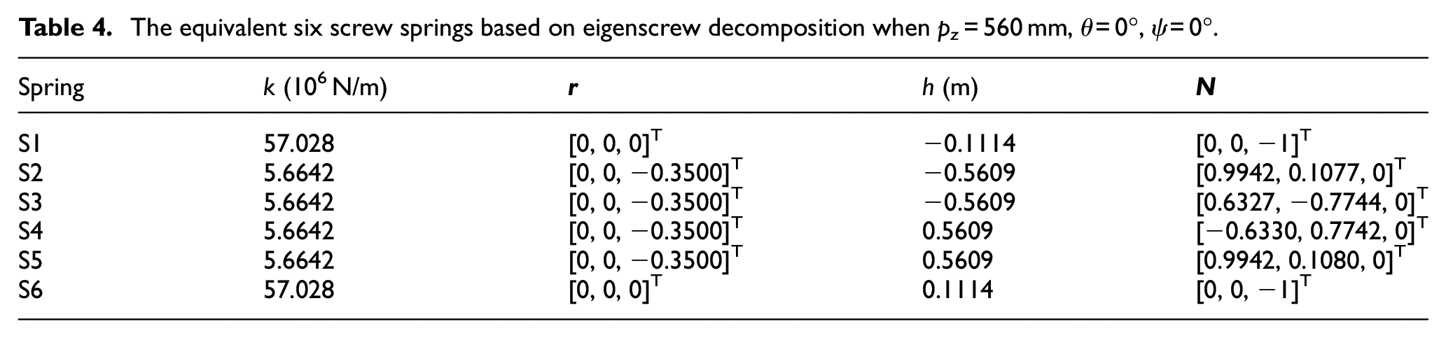
As can be seen from Table 3, there exists duality in the system. For example, the first column and the sixth column are dual to each other, meanwhile, the second column and the fifth column are dual to each other. The same rule can be found in Table 4. For example, there exist a dual pair between the first row and the sixth row.
The above eigenstiffnesses and eigenscrews can be converted into a physical description of screw springs with equivalent spring constants. This can be worked out with a parallel mechanism with six screw springs along the six eigenscrews as shown in Figure 11.
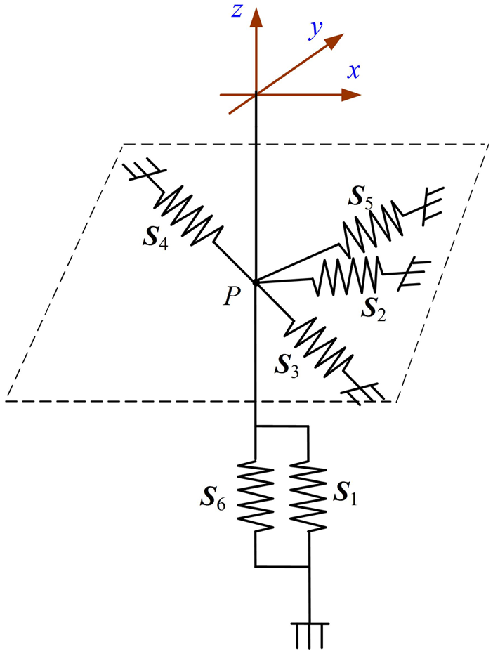
The physical interpretation of the stiffness of a 3-RPS PKM.
When a force produces a parallel linear deformation, and a rotational deformation about the action line produces a parallel couple, a compliant axis occurs. The existence of a compliant axis can also be judged from the eigenscrew solution. The sufficient and necessary condition for the occurrence of a compliant axis is given by the fact that there are two collinear eigenscrews with eigenstiffnesses of equal magnitude and opposite sign. The direction of the compliant axis is coincident with the direction of two collinear eigenscrews. 20 From Figure 11, it can be seen that there exists a compliant axis along the z-axis. The two collinear eigenscrews are in the direction of [0, 0, −1]T that is, minus the z-axis direction, with eigenstiffnesses of −1.2709 × 10⁻⁷ and 1.2709 × 10⁻⁷ N, respectively. The existence of the compliant axis indicates that the translation along the z-axis is an independent coordinate of the PKM, which demonstrates that one force along the z-axis only arouses a translational displacement along the z-axis while one moment about the z-axis arouses a rotational displacement about the z-axis.
Stiffness evaluation
Global stiffness prediction
To achieve desirable machining accuracy, a PKM module must possess a high rigidity throughout its workspace. Since the stiffness of the 3-RPS PKM is configuration-dependent, a designer may naturally propose that the minimum stiffness should be larger than a specified value throughout the workspace. In addition, the maximal value and average value of the stiffness throughout the workspace should address attentions for optimal design. Therefore, the minimum and maximum as well as the average spring constants of the proposed stiffness matrix are chosen as stiffness indices in order to have a global view of the stiffness performance of the PKM over the whole workspace.
In order to evaluate the stiffness performance throughout the workspace in a quick manner, a numerical approach is applied. The main concept of the numerical simulation is the partition of the whole workspace into discrete sampling pieces which are parallel to z-plane but with different z Cartesian coordinates and the piece-by-piece calculation of the three stiffness indices through eigenstiffness decomposition.
Figure 12 illustrates the distributions of the minimum, maximum and average stiffnesses of the PKM over the work plane at pz = 560 mm.
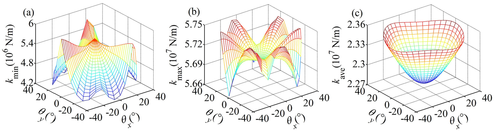
Distributions of stiffness indices throughout the working plane at pz = 560 mm (θx = θ sin ψ,θy = θ cos ψ): (a) minimum stiffness, (b) maximum stiffness and (c) average stiffness.
From Figure 12, it can be easily observed that the three stiffness indices of the 3-RPS PKM are axisymmetric, that is, 120° symmetrical about the axial direction of P joints over the given x–y work plane, which is coincident with the axial symmetry of three RPS limbs in the 3-RPS PKM.
Observations also imply a strong dependency of stiffness characteristics of the PKM on the mechanism’s configurations. As can be seen, the minimum of spring constants kmin varies from the lowest value of 4.259 × 10⁶ N/m to the highest value of 5.960 × 10⁶ N/m; the maximum of spring constants kmax changes from 5.663 × 10⁷to 5.745 × 10⁷ N/m and the vary interval of the average spring constant kave is [2.279 × 10⁷, 2.353 × 10⁷] N/m.
Further observations reveal that the lowest value of the minimum stiffness occurs at the boundary of the workspace when the moving platform reaches its maximum rotation angle where θx = −6.2674° and θy = −39.5075°, while that of the maximum stiffness occurs when θx = −40° and θy = 0°. Different from the maximum and minimum stiffnesses, the lowest value of the average stiffness occurs at the center of the workspace where θx = θy = 0° and kave = 2.279 × 10⁷ N/m.
Since the configuration parameters pz (or stroke s), the rotation angle θ and precession angle ψ are mainly determined by the working task requirements, the following will analyze the effects of dimensional parameters as well as structural parameters on the stiffness characteristics of the PKM.
Dimensional parameter effect on stiffness indices
Figure 13 shows the variations of the minimum stiffness kmin, maximum stiffness kmax and average stiffness kave with respect to the radii of the moving platform and base. Herein, the radius of the moving platform rp and that of the fixed base rb vary from 0.20 to 0.35 m, respectively.
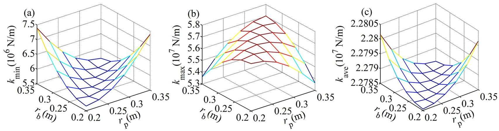
Variations of stiffness indices with respect to rp and rb: (a) minimum stiffness, (b) maximum stiffness and (c) average stiffness.
It can be easily observed from Figure 13 that the distributions of kmin, kmax and kave are symmetric about the plane of rp = rb, which means that the two-dimensional parameters rp and rb have the same “intensity” on the stiffness properties of the PKM design. However, the effects of dimensional parameters on the stiffness indices are different about the symmetry plane in that kmax decreases monotonously with the increment of rp and rb while kmin and kave increase monotonously with the increment of rp and rb. With this observation, it might be applaudable to take a strategy of rp = rb during the conceptual design stage for this kind of PKM design. Moreover, compared to the minimum and maximum stiffnesses, the effect of the dimensional parameter is very small for the interval of the average stiffness kave is [2.2786 × 10⁷, 2.2802 × 10⁷] N/m.
Structural parameter effect on stiffness indices
As aforementioned, the compliance of an individual limb assembly consists of compliances of limb body, the revolute joint and the spherical joint. Thus, the stiffness indices vary with physical parameters of the limb body directly, which affects the stiffness properties of the PKM in turn. Therefore, the following will analyze the effect of cross-sectional parameters of the limb body on the global stiffness indices.
For the convenience of analysis, some physical quantities are defined. For example, define a non-dimensional factor λkmin = kmin/kmin0, where kmin0 is the minimum stiffness of the example system when pz = 560 mm and θx = θy = 0°. In a similar way, λkmax and λkave are defined λkmax = kmax/kmax0, λkave = kave/kave0. Figure 14 shows the variations of three non-dimensional factors λkmin, λkmax and λkave with respect to δ. Herein, δ denotes the variation of cross sections as shown in Figure 3, that is, the diameters of cross sections I and IV, the length and width of cross sections II and III. It is noted that all the cross sections should be changed with a same variation δ simultaneously.
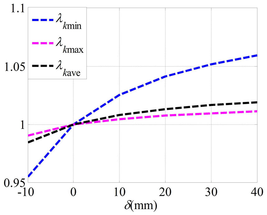
Variations of stiffness indices with respect to δ.
From Figure 14, it can be found that the three stiffness indices increase monotonously with the increment of cross sections. For clarity, the intervals of λkmin, λkmax and λkave are [0.9552, 1.0594], [0.9906, 1.0112] and [0.9847, 1.0192]. This is coincident with the common physical explanation, that is, a larger cross section of the limb body helps to improve the rigidity of the limb and thus, in turn, increases the rigidity of the whole PKM system. Comparing the three variation curves, one can find that the limb cross sections have a greater influence on the minimum stiffness kmin of the PKM design for its large variation.
From Figure 14, it seems that an effective way to improve the rigidity of the PKM is to adjust or optimize the dimension of the limb cross sections. However, it is worthy to point out that increasing the limb cross sections will definitely increase the weight and profile of the PKM and may rise other problems such as mechanical interference, which should be considered thoroughly at the design stage.
From the above analysis on Figures 13 and 14, both dimensional parameters and structural parameters have an important effect on the enhancement of the system rigidity. However, the changes in design variables also lead to the changes in dynamics. This may affect the dynamic performance of the PKM when it is applied for high-speed milling, which will be discussed in-depth in our other research article.
Conclusion
A hybrid modeling methodology was proposed to establish an analytical stiffness model for a novel 3-RPS PKM module. With this stiffness model, the rigidity performance of the 3-RPS PKM throughout its workspace was predicted in a quick manner by using a workspace partition algorithm. Based on the proposed model and stiffness analysis, the following conclusions can be drawn: (1) by using a combining method of VJM and FE formulation, the compliances of joints and limbs can be analytically formulated into the stiffness model, making it much more succinct than a numerical stiffness model. (2) The mapping of platform’s stiffness over the working envelope is strongly position-dependent and demonstrates a 120° symmetry about the z-axis, which is coincident with the structure features of the 3-RPS PKM. (3) The calculation errors of stiffness values between the analytical results and experimental tests are all less than 10% for different PKM’s configurations, implying the proposed model can be used to predict the stiffness properties of the 3-RPS PKM throughout its workspace with satisfactory accuracy. (4) In order to have an in-depth understanding of the platform’s rigidity, the stiffness matrix of the platform was extracted from the global stiffness matrix and physically interpreted as a rigid body suspended by six screw springs with equivalent stiffness constants and pitches through eigenscrew decomposition. (5) The parametric analysis indicates that the radii of the platform and the base have the same intensity on the platform’s stiffness while an optimal stiffness can be achieved by adjusting the limb cross sections.
Readers should note that the effects of the gravity, frictions and dampings are not included in this model, which, however, can be easily incorporated into the stiffness model with few efforts. In addition, readers may be aware that the present stiffness model can be further expanded as an elastodynamic model to perform dynamic analysis. These investigations are underway and will be presented elsewhere in the near future.
Footnotes
Appendix 1
Declaration of conflicting interests
The author(s) declared no potential conflicts of interest with respect to the research, authorship and/or publication of this article.
Funding
The author(s) disclosed receipt of the following financial support for the research, authorship, and/or publication of this article: This research was jointly supported by National Natural Science Foundation of China (Grant No. 51375013), Anhui Provincial Natural Science Foundation (Grant No. 1208085ME64), Open Research Fund of Key Laboratory of High Performance Complex Manufacturing, Central South University (Grant No. Kfkt2013-12), Open Fund of Shanghai Key Laboratory of Digital Manufacture for Thin-walled Structures (Grant No. 2014002) and State Key Laboratory for Manufacturing Systems Engineering (Xi’an Jiaotong University) (Grant No. sklms2015004). The corresponding author would like to thank the sponsor of China Scholarship Council (CSC, Grant No. 8260121203065).