Sage Journals: Discover world-class research

Abstract

The essence of the “ratio data” in cellular manufacturing system has rarely been correctly emphasized since past few decades of research and study. This article is an attempt to deal with cell formation problem which exploits machine utilization percentage and eliminates the “fuzziness” on the subject of ratio data. In the course of this study, a distinctive technique is adopted based on multi-criteria decision technique with significant modifications which is experimented on test data and compared with published methodology. To verify the grouping result, a novel performance measure is proposed and elaborated analytically to establish its superiority and robustness over the earlier efficiency measures published in the past literature of cellular manufacturing system. The novelty of this research remains in eradicating ambiguities on the subject of “ratio data,” imposing appropriate rules while generating the test problems, catering a unique multi-criteria decision technique–based approach and a novel performance measure for the aforesaid problem.

Keywords

Machine utilization percentage ratio data multi-criteria decision technique analytical hierarchy process cellular manufacturing system performance measure

Introduction

Cellular manufacturing system (CMS) is a function of group technology (GT), a manufacturing philosophy, which minimizes setup time, lead time, lot sizes, throughput and material handling cost, which further minimizes the level of the work-in-progress (WIP) and finished goods stocks in order to increase the utilization of the machines of the whole system.¹ CMS usually groups dissimilar machines into cells and similar parts into part families. Part families are then assigned to the appropriate cells depending upon their processing requirements which further enhance the total production of the system. This problem is universally known as cell formation problem (CFP) or machine-part grouping problem (MPGP). The very first step of CFP/MPGP is to acquire the near-best solution of the problem which is known as a combinatorial optimization problem which might be having numerous solutions in polynomial time (non-deterministic polynomial (NP)-complete).² In the past literature, the CFP/MPGP is presented with a matrix, namely, “machine-part incident matrix” (MPIM) in which all the elements are either 0 or 1 depending upon whether a particular part is being processed or not by a particular machine. This matrix data representation is known as “binary data.” Variations are found in such matrix data representations. If the unit processing time of parts is provided instead of the 1s’, then this is termed as “ratio data” and if the machining sequences of the parts are presented in the matrix, then this is named as “ordinal data.”³

Binary cell formation is the mostly used problem in the literature of CMS. McCormick et al.,⁴ Rajagopalan and Batra,⁵ King,⁶ Chandrasekharan and Rajagopalan,⁷ Srinivasan,⁸ Dimopoulos and Mort,⁹ Xambre and Vilarinho,¹⁰ Durán et al.,¹¹ Sayadi et al.¹² and so on are few of these. However, it is already a proven fact that binary cell formation only indicates the processing requirements, and in realistic production situation, cell formation implies far more than only processing requirements. These are processing time, processing sequence, machine utilization, production volume, available machining hours, machine breakdown time and many more.¹³ Yet researchers are working with 0–1 CFP till present time, which is merely significant in practice at present.¹⁴ The usage of ordinal data is being intensified in latest research of CMS.^15–18

Ratio data are considered in this research which are proposed by Venugopal and Narendran³ and being used since then.^13,19,20 George et al.¹⁹ have stated that the workload data are usually considered as ratio data in CMS, and an altered machine-part matrix is obtained using this information. The overall processing time of the job could be obtained when the total production volume and the processing time per unit are multiplied. All the “1”s in the incidence matrix are replaced with ratio values. The ratio data are finally obtained in the range of 0–1. However, authors did not particularly mention the procedure to achieve the workload ratio value (fractional figure) from total processing time data. Therefore, all the workload datasets found in the literature of CMS suffer from the lack of consistency which is further elaborated in section “Problem definitions.”

CFPs are primarily based on part coding analysis (PCA) and production flow analysis (PFA) among which PFA is mostly exploited which is based on job routing sheet rather than the shape and geometry of the parts. All the different variants of CFPs are being solved using numerous published methods, which are classified as array-based method, clustering methods, similarity coefficient–based methods, graph partitioning techniques, mathematical programming (MP) approaches and soft computing (SC) methods.²¹

Array-based approaches count binary words which are presented by the rows and columns of the 0–1 matrix and adjust them in such a way that these would convert the matrix into another matrix where non-zero elements are diagonally arranged in blocks. To solve the CFPs, the use of rank order clustering (ROC) technique is moderately higher than the other array-based methods.⁶ Chandrasekharan and Rajagopalan⁷ and King and Nakornchai²² have modified the ROC technique further to obtain adjusted and enhanced solutions in CMS. Other important array-based methodologies are direct clustering analysis recommended by Chan and Milner²⁴ and bond energy algorithm introduced by McCormick et al.⁴

Generalized clustering approaches are being used in CMS with or without modifications to achieve machine-part cells since past few decades. Clustering methods could be categorized into (1) hierarchical techniques and (2) non-hierarchical techniques primarily. Among these, bond energy algorithm by McCormick et al.,⁴ ROC by King,⁶ modified ROC by Chandrasekharan and Rajagopalan⁷ and King and Nakornchai,²² hierarchical clustering approach by Dimopoulos and Mort,⁹ heuristic-based clustering method by Waghodekar and Sahu,²³ direct clustering approach by Chan and Milner,²⁴ matrix-based clustering approach by Kusiak,²⁵ non-hierarchical clustering approach by Srinivasan and Narendran,²⁶ generalized approach by Seifoddini,²⁷ hierarchical approach based on similarity and distance metrics by Shafer and Rogers²⁸ and improved method over ROC by Mosier and Taube²⁹ are the most popular clustering methods which are being widely practiced in CMS.

Similarity coefficient–based approaches are first reported by McAuley.³⁰ These methods exploit the similarity between two machines and put them in same or different cells based on their composite score of similarity. Some articles depict the reverse technique and compute dissimilarity coefficient scores among machines and put them in cells based on the scores achieved. Prabhakaran et al.³¹ stated dissimilarity coefficient for generalized CFPs which practically introduces the operation sequences (ordinal data) and operational time (ratio data) of components. Once the similarity/dissimilarity scores are acquired, some suitable clustering techniques are employed to form a hierarchical tree structure called dendrogram to obtain the cells, and such clustering methods could be based on single linkage clustering analysis (SLCA) by Dimopoulos and Mort⁹ or average linkage clustering analysis (ALCA) by Seifoddini and Wolfe.³²

In graph theory–based methods, machines are denoted as vertices (V) and the arcs’ weights (E) represent the machine similarities and the composite structure as G (V, E). Rajagopalan and Batra⁵ first recommended the practice of graph theoretic approach to obtain optimal manufacturing cells. Chandrasekharan and Rajagopalan⁷ suggested an ideal-seed non-hierarchical clustering approach which utilizes graph theory efficiently in CMS. Ballakur and Steudel³³ offered a graph searching algorithm which selects a pivot machine or part based on a pre-definite norm and forms the cells around the pivots. Minimum spanning tree (MST) for the CFP is used by Srinivasan.⁸ An MST of machines could be obtained in first stage and in later stage the part family seeds are spawned using previous MST. A graph theory–based NP-algorithm for optimal cell design termed as vertex-tree graphic matrices is developed by Veeramani and Mani.³⁴

Various MP methods are successfully practiced in the domain of CMS. Among these, integer linear programming (ILP) is used by Kusiak²⁵ and Rabbani et al.,³⁵ goal programming (GP) is proposed by Shafer and Rogers,²⁸ dynamic programming (DP) is practiced by Ballakur and Steudel³³ and linear programming (LP) is introduce by Boctor.³⁶ Ramabhatta and Nagi³⁷ proposed some branch-and-bound (B&B) technique to obtain block diagonal formation which minimizes inter-cell material flow considering complementary routings of the parts being processed. MP methods are extremely popular since these tools are highly capable of dealing with the real-life constraints and practical aims for manufacturing firms while obtaining ideal cellular structure on shop-floor. These techniques are two-phase techniques. In the first phase, the objectives and constraints of manufacturing firm are presented in the form of mathematical equations and inequalities, and in the latter phase, the model is solved using an appropriate optimization algorithm/tool.

Lately, the soft computing–based methods became hugely popular for solving the CFPs due to its proven ability of optimizing large and complex data, for example, Tabu search approach,^38,39 neural network,^40–42 genetic algorithms (GAs),^43–49 simulated annealing^10,50,51 and other latest nature-inspired algorithms such as particle swarm optimization (PSO),¹¹ ant algorithm,⁵² firefly-inspired algorithm¹² and bacteria foraging algorithm (BFA).⁵³ These techniques are capable of achieving better solutions; however, these are not reasonably quick in terms of central processing unit (CPU) time. Furthermore, the time complexity becomes higher with the increasing number of jobs and machines for the problem.

In this article, a typical CFP is demonstrated which employs machine utilization percentage as the major criterion of cell design. Thereafter, a novel machine-part ranking technique is adopted which is a multi-criteria decision technique (MCDT) model based on analytical hierarchy process (AHP). This technique is considerably modified using machine utilization percentage as an important factor. This proposed methodology is verified on few datasets and successfully compared with McQueen’s⁵⁴ K-means method. To measure the goodness of the obtained solutions, a new performance measure called utilization-based grouping efficiency (UGE) based on machine usage is also proposed, and finally, an analytical study is presented on the UGE to establish its superiority and robustness over other published efficiency measures for ratio data.

The remainder of this article is prepared in the following order. Section “Problem definitions” would discuss the problem considered in this article. Section “AHP-based algorithm” demonstrates the methodology adopted in a systematic manner. Section “Performance measure” reports the detailed discussion on the new grouping measure UGE, section “Results and discussion” portrays the results acquired and analyzes the significance of the aimed approach and section “Conclusion” concludes this study.

Problem definitions

As per the stated ideas, many articles are authored in the domain of CMS, but very few of these particularly addressed the “processing time” or “ratio data” in practical and scientific manner. As it was first demonstrated by Venugopal and Narendran,³ the proposed problem is re-defined here in the following manner

u_{ij} = \frac{(t_{ij} \times n_{j})}{M H_{i}}

(1)

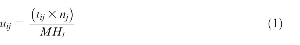
where t_ij is the unit processing time (hour/unit) of part j on machine i; 1 ⩽ i ⩽ q and 1 ⩽ j ⩽ p, n_j is the production volume of part j, MH_i is the available machine hours of machine i, U = [u_ij] is an (p × q)-machine-component incidence matrix where u_ij is the percentage utilization of machine i induced by part j.

Conditions imposed

u_{ij} = {\begin{matrix} z ero, if part j is not being processed by machine i \\ non zero, if part j is being processed by machine i \end{matrix}

(2)

For each part j

\sum_{j = 1}^{p} u_{ij} ⩽ 1

(3)

Equation (1) generates an MPIM U which is widely recognized as “processing time” matrix. However, the elements (u_ij) of matrix U do not indicate any absolute values; therefore, these should not be dubbed as “processing time” realistically. These values are percentage values (hours ÷ hours); hence, these are unit-less.

u_ij expresses the fraction of machine hours of machine i being utilized to produce the total volume of a particular part j on the machine i. Therefore, a novel idiom is adopted in this article, “percentage utilization of machine” or “machine utilization factor,” which is more sensible and relevant than “processing time.”

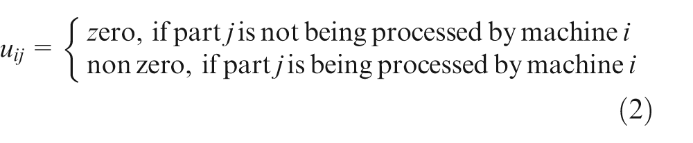
For that matter two conditions (equations (2) and (3)) are imposed on equation (1).

Condition 1

Equation (2) shows that value of u_ij is either zero or non-zero depending upon the processing requirement of a particular part j on a particular machine i.

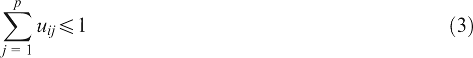
Condition 2

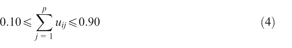
Equation (3) shows that the total percentage utilization of machine i for all parts must not be theoretically larger than 1 because the total utilization (TU) of a machine can never be more than 100%. However, in actual scenario, a particular machine is never being used for all the time as long as the shift runs on shop-floor. Therefore, total machine utilization for a particular machine remains in the range [0.1, 0.9] realistically and equation (3) is modified as

$0.10 ⩽ \sum_{j = 1}^{p} u_{ij} ⩽ 0.90$
(4)

Problem instance

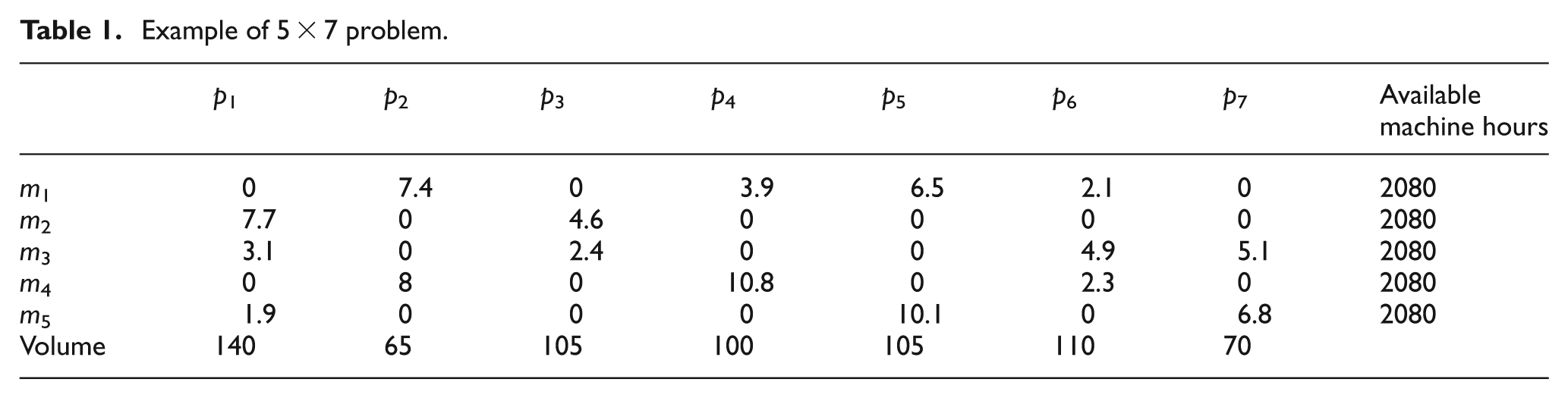
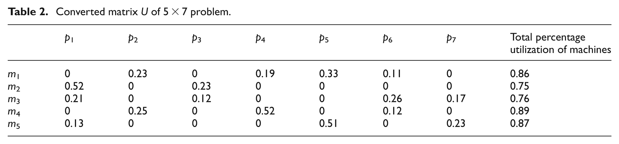
An example of the stated problem is depicted in Table 1 for five machines and seven parts with unit processing time (hour/unit), production volume and available machine hours. Using the stated method, the U matrix is obtained and shown in Table 2 satisfying all conditions.

Table 1.
Example of 5 × 7 problem.

p ₁ p ₂ p ₃ p ₄ p ₅ p ₆ p ₇ Available machine hours

m ₁ 0 7.4 0 3.9 6.5 2.1 0 2080

m ₂ 7.7 0 4.6 0 0 0 0 2080

m ₃ 3.1 0 2.4 0 0 4.9 5.1 2080

m ₄ 0 8 0 10.8 0 2.3 0 2080

m ₅ 1.9 0 0 0 10.1 0 6.8 2080

Volume 140 65 105 100 105 110 70

Table 2.
Converted matrix U of 5 × 7 problem.

p ₁ p ₂ p ₃ p ₄ p ₅ p ₆ p ₇ Total percentage utilization of machines

m ₁ 0 0.23 0 0.19 0.33 0.11 0 0.86

m ₂ 0.52 0 0.23 0 0 0 0 0.75

m ₃ 0.21 0 0.12 0 0 0.26 0.17 0.76

m ₄ 0 0.25 0 0.52 0 0.12 0 0.89

m ₅ 0.13 0 0 0 0.51 0 0.23 0.87

AHP-based algorithm

The AHP method used in this article is a multi-criteria decision approach (MCDA) which uses hierarchical relations among machines and parts to represent the CFP. AHP allows the decision makers to correspond to the crossing points of various factors in complex and uncertain scenario. In his pioneer work, Saaty⁵⁵ stated that the priorities for alternatives are obtained depending upon the viewpoints of the experts in the area of study. Assuming a CFP has q criteria (machines), m₁, m₂,…, m_q, and n alternatives (parts), p₁, p₂,…, p_n, every alternative is assessed relating to the q criteria. The said approach is grounded on the pairwise comparison of alternatives relating to the criteria. These pairwise comparison matrices could be attained (q × q), q is the number of comparing criteria. The adopted AHP algorithm is demonstrated herewith.

Step 1

The relational hierarchy of the 5 × 7 test problem (Table 1) is shown in Figure 1. The problem is dismantled into three levels:⁵⁵ The first level reports the primary objective: cell formation, the second level depicts the criteria (machines) and the third level portrays the alternatives (parts) to be compared.

Figure 1.
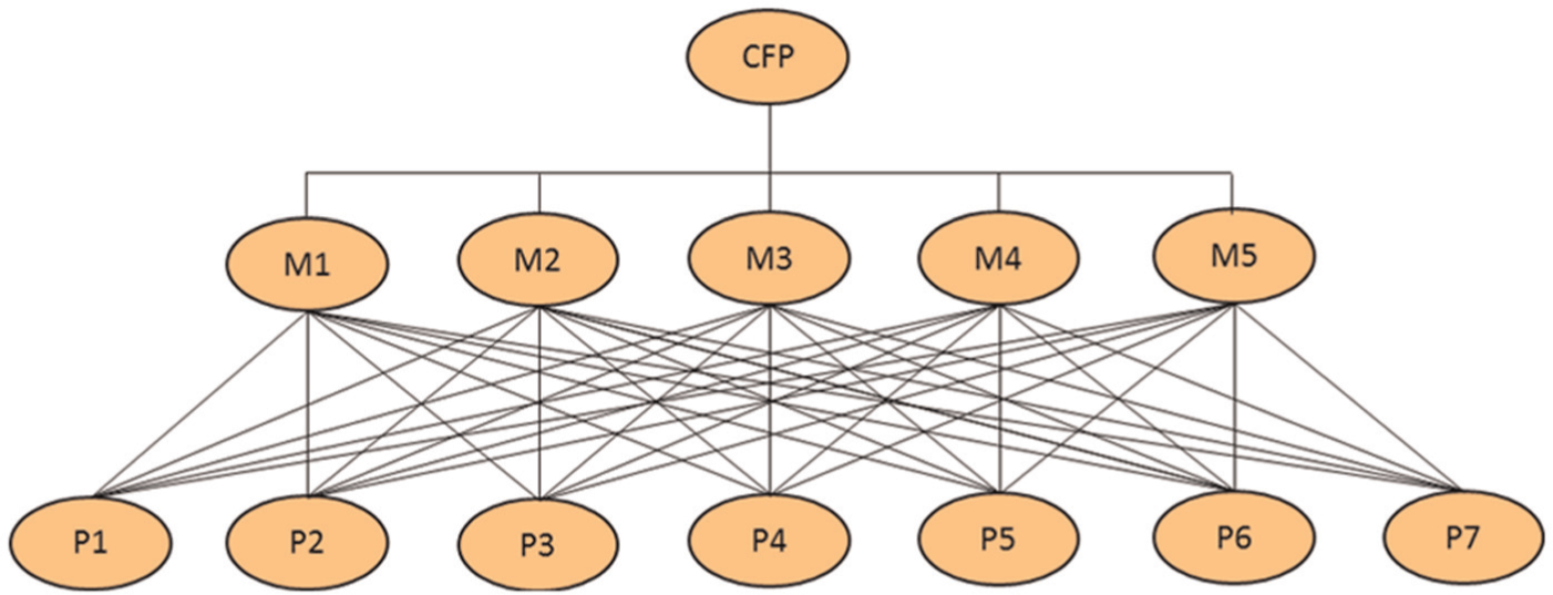
Relational hierarchy of the cell formation problem (CFP).

Step 2

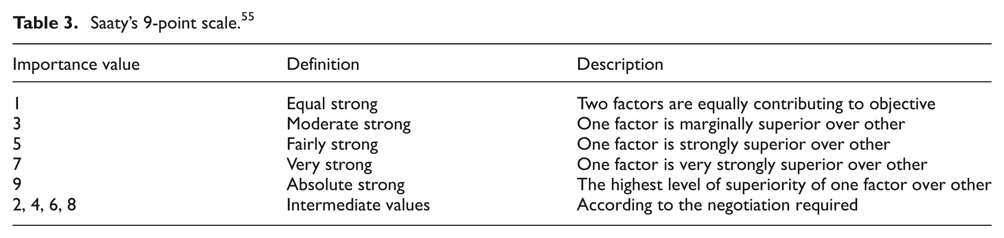
The pairwise comparison of each level can be obtained using computing formula provided in equations (5)–(9). To achieve this, a ranking scale is necessary for evaluation of criteria.⁵⁵ Saaty’s scale is portrayed in Table 3. To assign these values to the criteria, AHP questionnaire sheet is required on which experts’ opinion could be obtained. This implies that the qualitative factors are being converted into numerical values to ease the computation.

Table 3.
Saaty’s 9-point scale.⁵⁵

Importance value Definition Description

1 Equal strong Two factors are equally contributing to objective

3 Moderate strong One factor is marginally superior over other

5 Fairly strong One factor is strongly superior over other

7 Very strong One factor is very strongly superior over other

9 Absolute strong The highest level of superiority of one factor over other

2, 4, 6, 8 Intermediate values According to the negotiation required

The abovementioned phenomena cannot be directly adopted for MPGP. Therefore, substantial modification is performed in this article to adopt Saaty’s scale for CFP.

Step 2.1

For each machine i, the total percentage utilization is computed using

$T U_{i} = \sum_{j = 1}^{p} u_{ij}$
(5)

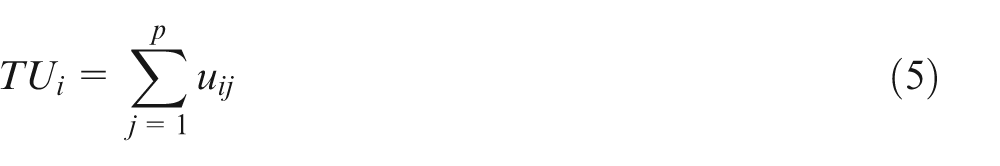
These values are listed in the last column of Table 2. According to the proposition of equation (4), these values remain between 0.1 and 0.9.

Step 2.2

The largest and smallest TU values are obtained from Table 2, and the “scaling factor for criteria” (σ_c) is obtained using equation (6)

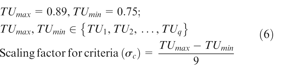
$\begin{matrix} T U_{\max} = 0.89, T U_{\min} = 0.75; \\ T U_{\max}, T U_{\min} \in {T U_{1}, T U_{2}, \dots, T U_{q}} \\ Scaling factor for criteria (σ_{c}) = \frac{T U_{\max} - T U_{\min}}{9} \end{matrix}$
(6)

For the example problem considered, the value of scaling factor (σ) is 0.02.

Step 2.3

At this point, the pairwise comparison matrix for criteria (q × q) is believed to be formed. For that matter, each criteria is believed to be compared with another. Here, this comparison is done using equation (7)

$d_{i {(i + 1)}^{c}} = \frac{T U_{i} - T U_{i + 1}}{σ}$
(7)

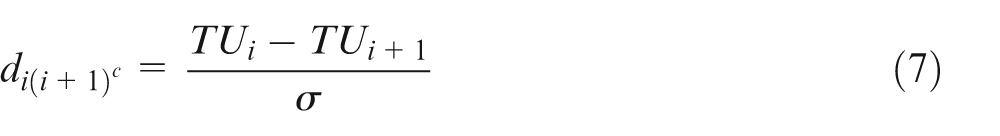
d_i_(i ₊ ₁₎^c is the distance between machine i and machine i + 1. This value is mapped with the modified Saaty’s scale suggested in Table 4.

Table 4.
Modified Saaty’s scale.

d_i_(i ₊ ₁₎ values Saaty’s value Definition

0–1 1 Equal strong

1–2.5 2 Intermediate values

2.5–3.5 3 Moderate strong

3.5–4.5 4 Intermediate values

4.5–5.5 5 Fairly strong

5.5–6.5 6 Intermediate values

6.5–7.5 7 Very strong

7.5–8.5 8 Intermediate values

8.5–rest 9 Absolute strong

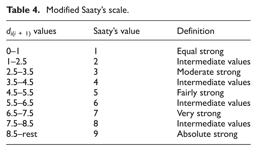
Thereafter, the pairwise comparison matrix is formed with all the d_i_(i ₊ ₁₎. If the value of d_i_(i ₊ ₁₎ is +ve, that is, machine i has more priority over machine i + 1 and if value of d_i_(i ₊ ₁₎ is −ve, that is, machine i + 1 has more priority over machine i. Using equation (7) and Table 4, the pairwise comparison matrix is obtained and depicted in Figure 2.

Figure 2.
Pairwise comparison matrix of criteria (machines).

Step 3

Calculation of the pairwise comparison matrix for all the alternatives (parts) with respect to each criterion (machine) is performed using a minute modification added with the prior step.

Step 3.1

The largest and smallest u_ij values are obtained from Table 2 and the scaling factor for alternatives (σ_a) is obtained using equation (8)

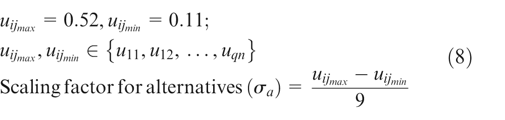
$\begin{matrix} u_{i j_{\max}} = 0.52, u_{i j_{\min}} = 0.11; \\ u_{i j_{\max}}, u_{i j_{\min}} \in {u_{11}, u_{12}, \dots, u_{qn}} \\ Scaling factor for alternatives (σ_{a}) = \frac{u_{i j_{\max}} - u_{i j_{\min}}}{9} \end{matrix}$
(8)

For the example problem considered, the value of scaling factor for alternatives (σ_a) is 0.05.

Step 3.2

At this point, the pairwise comparison matrices for alternatives (q × q) are believed to be formed. For that matter, each alternative is believed to be compared with another. Here, this comparison is done using equation (9)

$d_{j {(j + 1)}^{a}} = \frac{u_{ij} - u_{i (j + 1)}}{σ_{a}}$
(9)

d_j_(j ₊ ₁₎^a is the distance between part j and part j + 1 for every machine i. This value is mapped with the modified Saaty’s scale suggested in Table 4.

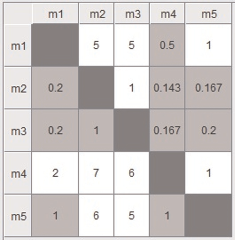
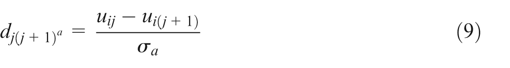
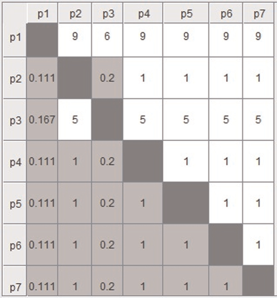
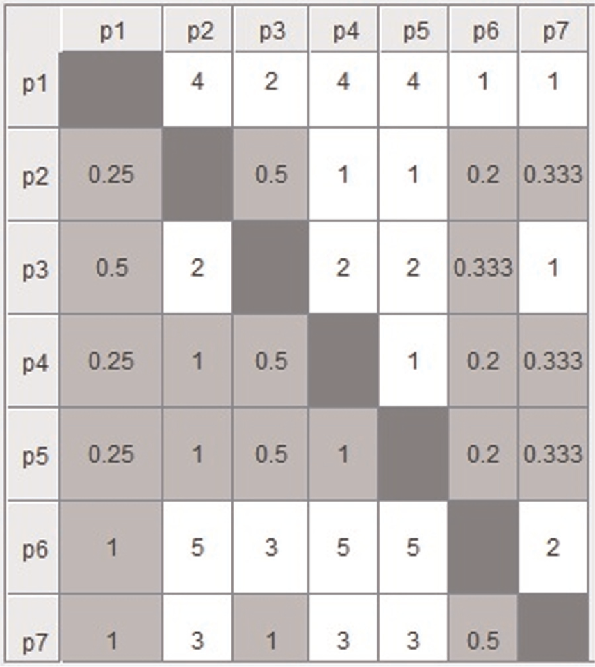
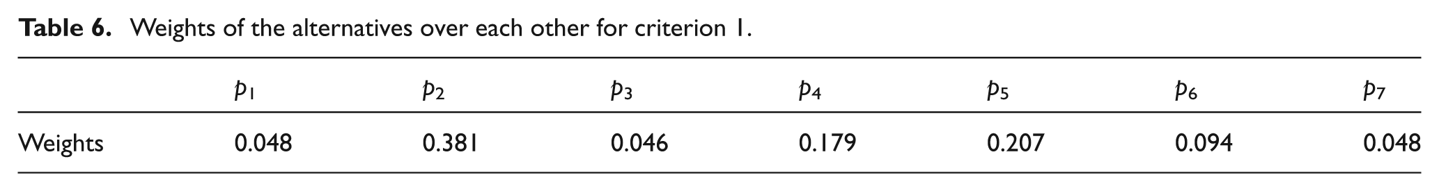
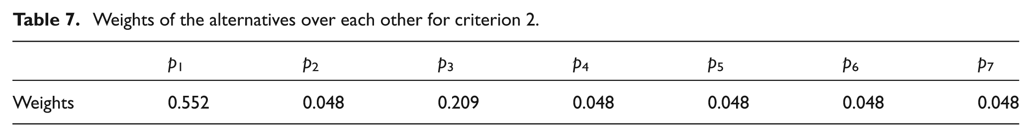
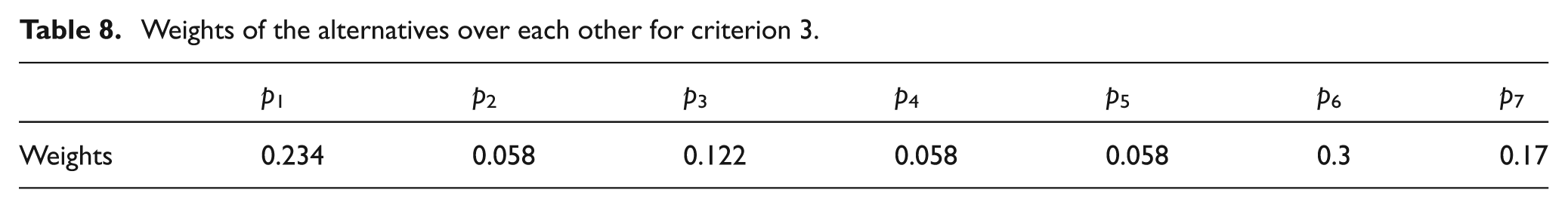
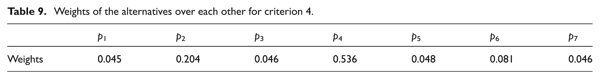
Thereafter, the pairwise comparison matrices are formed with all the d_j_(j ₊ ₁₎. If the value of d_j_(j ₊ ₁₎ is +ve, that is, part j has more priority over part j + 1 and if value of d_j_(j ₊ ₁₎ is −ve, that is, part j + 1 has more priority over part j. Using equation (9) and Table 4, the pairwise comparison matrix for every criterion (machine) is obtained and depicted in Figures 3 –7.

Figure 3.
Pairwise comparison matrix of alternatives (parts) for criterion 1 (machine 1).

Figure 4.
Pairwise comparison matrix of alternatives (parts) for criterion 2 (machine 2).

Figure 5.
Pairwise comparison matrix of alternatives (parts) for criterion 3 (machine 3).

Figure 6.
Pairwise comparison matrix of alternatives (parts) for criterion 4 (machine 4).

Figure 7.
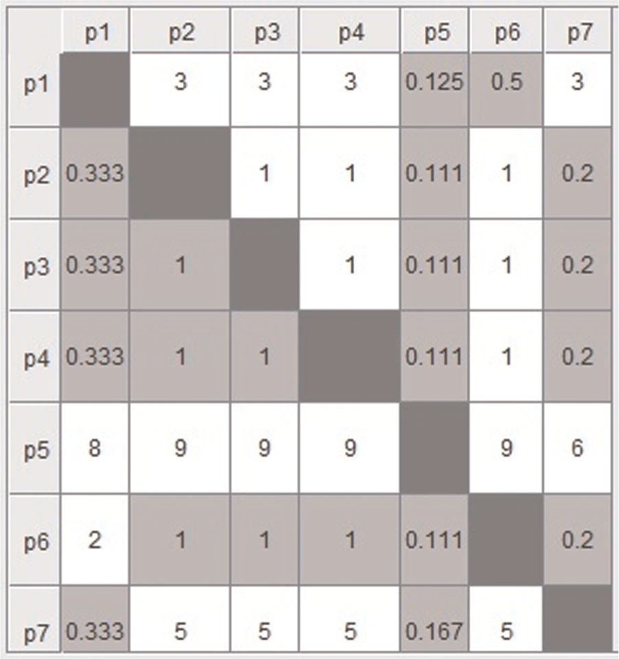
Pairwise comparison matrix of alternatives (parts) for criterion 5 (machine 5).

Step 4

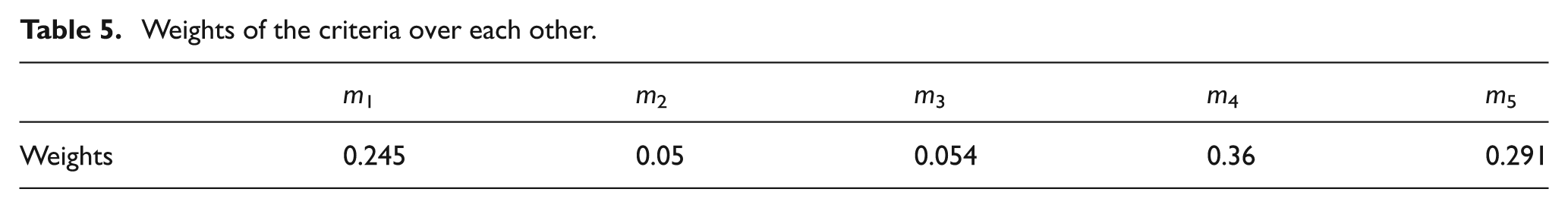
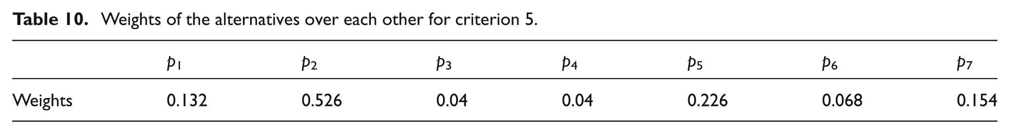
Once all the pairwise comparison matrices are obtained, a generic AHP computing algorithm is applied and the respective relative weights for each matrix is obtained and presented in Tables 5 –10.

Table 5.
Weights of the criteria over each other.

m ₁ m ₂ m ₃ m ₄ m ₅

Weights 0.245 0.05 0.054 0.36 0.291

Table 6.
Weights of the alternatives over each other for criterion 1.

p ₁ p ₂ p ₃ p ₄ p ₅ p ₆ p ₇

Weights 0.048 0.381 0.046 0.179 0.207 0.094 0.048

Table 7.
Weights of the alternatives over each other for criterion 2.

p ₁ p ₂ p ₃ p ₄ p ₅ p ₆ p ₇

Weights 0.552 0.048 0.209 0.048 0.048 0.048 0.048

Table 8.
Weights of the alternatives over each other for criterion 3.

p ₁ p ₂ p ₃ p ₄ p ₅ p ₆ p ₇

Weights 0.234 0.058 0.122 0.058 0.058 0.3 0.17

Table 9.
Weights of the alternatives over each other for criterion 4.

p ₁ p ₂ p ₃ p ₄ p ₅ p ₆ p ₇

Weights 0.045 0.204 0.046 0.536 0.048 0.081 0.046

Table 10.
Weights of the alternatives over each other for criterion 5.

p ₁ p ₂ p ₃ p ₄ p ₅ p ₆ p ₇

Weights 0.132 0.526 0.04 0.04 0.226 0.068 0.154

Hence, the generic AHP algorithm to compute relative weights is stated hereunder as presented by Ghosh et al.⁵⁶ Consider [B_y = λ_maxy] where B is the comparison (m × m), where m is the number of criteria; y denotes the Eigenvector (m × 1); and λ_max is the Eigenvalue, λ_max ∈ ℜ > m.

Eigenvector Y can be obtained using the following algorithm:

1. Initialization:

1.1. matrix B is multiplied with the same to obtained square matrix, that is, B² = B × B

1.2. Sums of rows of B² are obtained which is further normalized to find E₀.

1.3. Assign B: = B²

2. Main:

2.1. matrix B is multiplied with the same to obtained square matrix, that is, B² = B × B

2.2. Sums of rows of B² are obtained which is further normalized to find E₁.

2.3. Obtain D = E₁ − E₀.

2.4. If all the elements of D are near to zero value, assign Y = E₁

2.5. else assign B: = B², assign E₀: = E₁ and go to Step 2.1.

2.6. STOP.

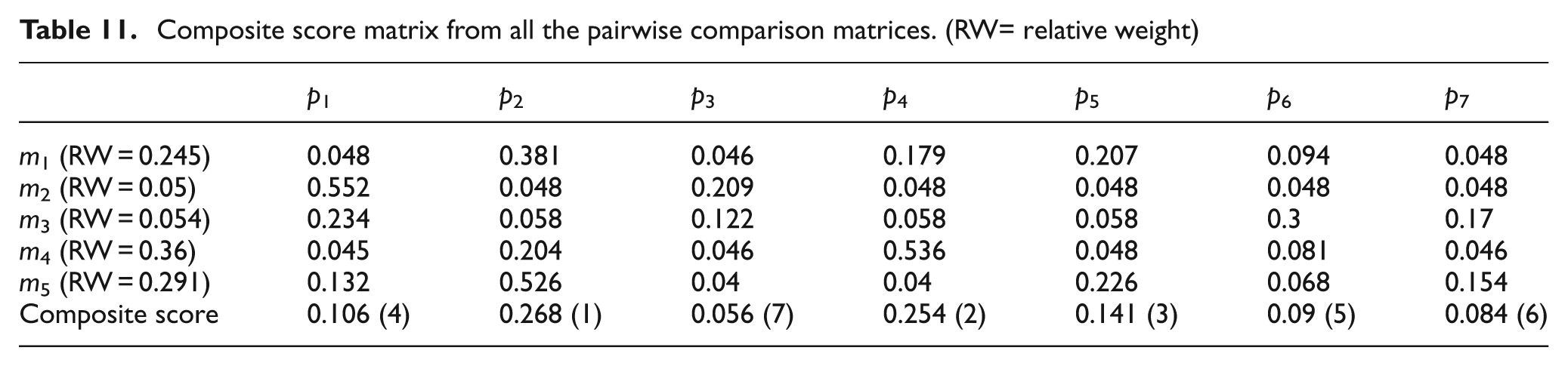
Thereafter, relative weight factor obtained for each criterion and the alternatives are multiplied. Then, the total rating of each alternative is calculated by adding these obtained values (Table 11). Table 11 demonstrates that part 2 is the highest ranked part with composite ranking “1” and composite score “0.268” followed by parts 4, 5, 1, 6, 7 and 3.

Table 11.
Composite score matrix from all the pairwise comparison matrices. (RW= relative weight)

p ₁ p ₂ p ₃ p ₄ p ₅ p ₆ p ₇

m₁ (RW = 0.245) 0.048 0.381 0.046 0.179 0.207 0.094 0.048

m₂ (RW = 0.05) 0.552 0.048 0.209 0.048 0.048 0.048 0.048

m₃ (RW = 0.054) 0.234 0.058 0.122 0.058 0.058 0.3 0.17

m₄ (RW = 0.36) 0.045 0.204 0.046 0.536 0.048 0.081 0.046

m₅ (RW = 0.291) 0.132 0.526 0.04 0.04 0.226 0.068 0.154

Composite score 0.106 (4) 0.268 (1) 0.056 (7) 0.254 (2) 0.141 (3) 0.09 (5) 0.084 (6)

Machine ranking method

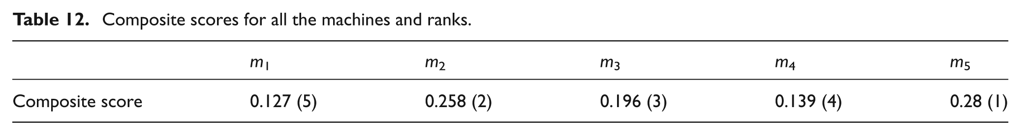
Subsequently, the machines are ranked using the identical technique. For that matter, the machines are assigned as alternatives and the parts are assigned as criteria. After the composite score computation, the machine ranks are obtained and demonstrated in Table 12. Table 12 demonstrates that machine 5 (overall ranking is 1 and composite score is 0.28) is the highest ranked machine followed by machines 2, 3, 4 and 1.

Table 12.
Composite scores for all the machines and ranks.

m ₁ m ₂ m ₃ m ₄ m ₅

Composite score 0.127 (5) 0.258 (2) 0.196 (3) 0.139 (4) 0.28 (1)

Finalizing the cell formation solution

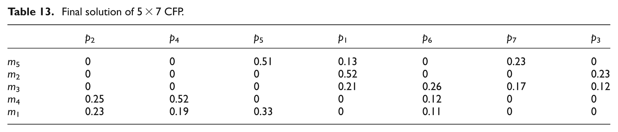
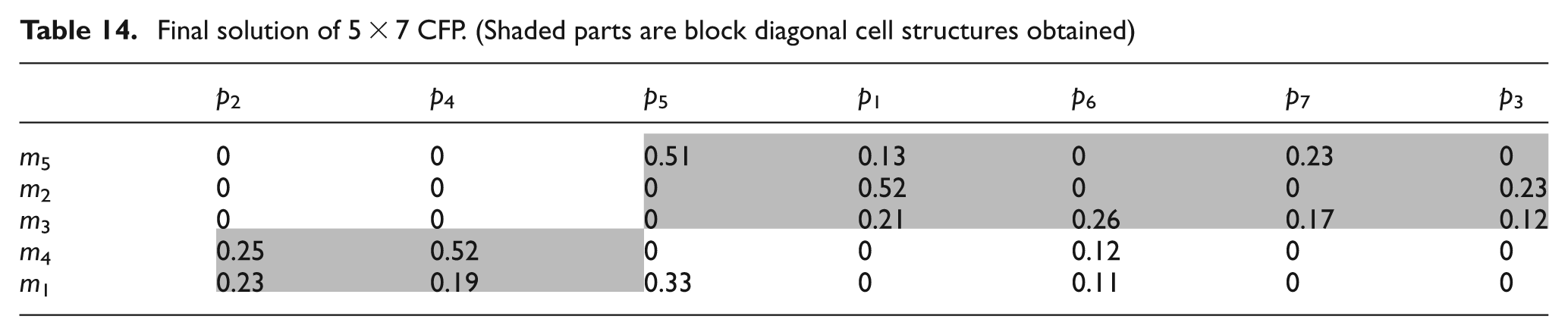
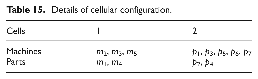
In the final step, the machines and parts of the initial CFP that are obtained in Table 2 are ordered with their ranks obtained from Tables 11 and 12. This newly formed ordered machine-part incidence matrix is portrayed in Table 13. The block diagonal structure which indicates the group of machines and parts in cells can be used to determine the cellular structure. For the present 5 × 7 problem, the block diagonal cellular structure is depicted in Table 14 and the details of the cells are shown in Table 15.

Table 13.
Final solution of 5 × 7 CFP.

p ₂ p ₄ p ₅ p ₁ p ₆ p ₇ p ₃

m ₅ 0 0 0.51 0.13 0 0.23 0

m ₂ 0 0 0 0.52 0 0 0.23

m ₃ 0 0 0 0.21 0.26 0.17 0.12

m ₄ 0.25 0.52 0 0 0.12 0 0

m ₁ 0.23 0.19 0.33 0 0.11 0 0

Table 14.
Final solution of 5 × 7 CFP. (Shaded parts are block diagonal cell structures obtained)

p ₂ p ₄ p ₅ p ₁ p ₆ p ₇ p ₃

m ₅ 0 0 0.51 0.13 0 0.23 0

m ₂ 0 0 0 0.52 0 0 0.23

m ₃ 0 0 0 0.21 0.26 0.17 0.12

m ₄ 0.25 0.52 0 0 0.12 0 0

m ₁ 0.23 0.19 0.33 0 0.11 0 0

Table 15.
Details of cellular configuration.

Cells 1 2

Machines m₂, m₃, m₅ p₁, p₃, p₅, p₆, p₇

Parts m₁, m₄ p₂, p₄

Performance measure

According to the past literature, there are two mostly explored measures are grouping efficiency by Chandrasekharan and Rajagopalan⁷ and grouping efficacy by Kumar and Chandrasekharan⁵⁷, which are heavily being used to verify the clustering efficiency of machine cells obtained by an appropriate grouping method. However, these two measures do not work with ratio data since these are designed for binary data. Therefore, these measures are incapable to handle CFPs with percentage utilization of machines. Generalized grouping efficacy developed by Zolfaghari and Liang⁴⁴ is designed to handle CFPs where ratio data are considered. However, generalized grouping efficacy overlooks the influence of voids in the machine cells, which primarily affects the quality of the solutions obtained for CFPs. For that matter, Ponnambalam et al.⁵⁸ proposed another performance measure which suitably deals with ratio data–based CFP and considered exceptional elements and void efficiently. This measure is known as modified grouping efficiency (MGE)

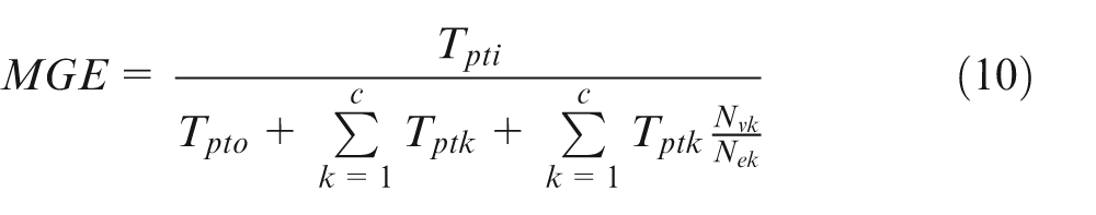
$MGE = \frac{T_{pti}}{T_{pto} + \sum_{k = 1}^{c} T_{ptk} + \sum_{k = 1}^{c} T_{ptk} \frac{N_{vk}}{N_{ek}}}$
(10)

where T_pti is the total processing time inside the cells, T_pto is the total processing time outside the cells, T_ptk is the total processing time of cell k, N_vk is the no. of voids in cell k and N_ek is the total number of elements in cell k.

However, MGE is capable of checking the effect of the number of exceptional elements only, but it fails to investigate the influence of the numerical values (percentage utilizations) of the exceptional elements. Hence, a novel performance measure for CFP dubbed as UGE has been introduced in this article that competently deals with percentage utilization (ratio data) matrix with all the facts ignored in all the previously published performance measures.

Few rules are believed to be considered while designing an efficient grouping measure for the ratio data–based CFP. These rules are as follows:

Rule 1. The holistic utilization of all the machines in the whole plant is always constant. This numerical figure is substantially significant while designing a performance measure.

Rule 2. Number of voids and exceptional elements should be integrated in the design.

Rule 3. Consideration of utilization of each individual cell is important since presence of voids influences the cumulative in-cell utilizations.

Rule 4. The ratio of the utilization of all the exceptional elements and the total in-cell utilization should be incorporated in design which not only considers the number of exceptional elements but also the utilization (numerical figure) of exceptional elements.

Following all the rules described, the new performance measure UGE is proposed in this article. The UGE is defined using following equation (11)

$UGE = \frac{(\sum_{k = 1}^{c} [U_{cell}^{k} (1 - \frac{V_{k}}{E_{k}})]) (1 - \frac{U_{ee}}{\sum_{k = 1}^{c} U_{cell}^{k}})}{U_{plant}}$
(11)

$U_{cell}^{k} = {\sum_{i = 1}^{mic} \sum_{j = 1}^{pic} u_{ij}}^{k}$
(12)

$U_{ee} = \sum_{i = 1}^{moc} \sum_{j = 1}^{poc} u_{ij}$
(13)

$U_{plant} = \sum_{i = 1}^{mtp} \sum_{j = 1}^{ptp} u_{ij}$
(14)

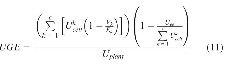
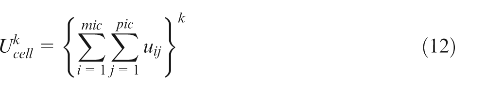
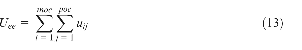
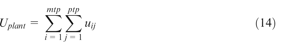
where c is the number of cells, m is the number of parts, p is the number of machines, k is the index of cell {k = 1, 2,…, c}, i is the index of machines {i = 1, 2,…, m}, j is the index of parts {i = 1, 2,…, p}, $U_{cell}^{k}$ is the total utilization of kth cell, U_plant is the total utilization of plant, U_ee is the total utilization outside the block diagonal cell structure, u_ij is the utilization of machine i induced by part j; 1 ⩽ i ⩽ q and 1 ⩽ j ⩽ n, V_k is the total number of voids in cell k {k = 1, 2,…, c}, E_k is the total number of elements in cell k {k = 1, 2,…, c}, mic is the number of machines in cell, pic is the number of parts in cell, moc is the number of machines outside of cells, poc is the number of parts outside of cells, mtp is the total number of machines in plant and ptp is the total number of parts in plant.

Due to the qualitative differences among various performance measures, some suitable sensitivity analysis and a qualitative analysis are required⁵⁹ to authenticate this newly developed performance measure. Hence, the following discussion would depict the in-depth comparison among UGE and its nearest predecessor MGE. It would also be portrayed that all the facts which are ignored while designing MGE are accomplished in UGE.

Sensitivity analysis

To assess the sensitivity of UGE and MGE with the variations of datasets and the goodness of block diagonal cell structure obtained in solution matrix, different versions of the 5 × 7 CFP of Table 2 are considered. Deviations from one version to another are restricted to small amount of changes in the number of exceptional elements and their utilization factors.

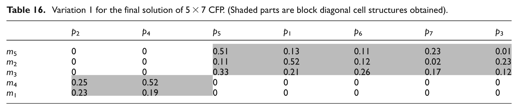
The solution matrix obtained in Table 14 has three exceptional elements and six voids. Variation 1 is shown in Table 16, part 6 is no longer being process through machine 4 and machine 1 rather being processed through machine 2 and machine 5 and part 5 is being processed through machine 3 instead of being processed through machine 1. It is a compact or ideal CFP solution (no exceptional elements and no voids), obtained by replacing all three voids of variation 1 with arbitrary utilization values. As per the norms of efficiency measures, both MGE and UGE show 100% values for this configuration.

Table 16.
Variation 1 for the final solution of 5 × 7 CFP. (Shaded parts are block diagonal cell structures obtained)

p ₂ p ₄ p ₅ p ₁ p ₆ p ₇ p ₃

m ₅ 0 0 0.51 0.13 0.11 0.23 0.01

m ₂ 0 0 0.11 0.52 0.12 0.02 0.23

m ₃ 0 0 0.33 0.21 0.26 0.17 0.12

m ₄ 0.25 0.52 0 0 0 0 0

m ₁ 0.23 0.19 0 0 0 0 0

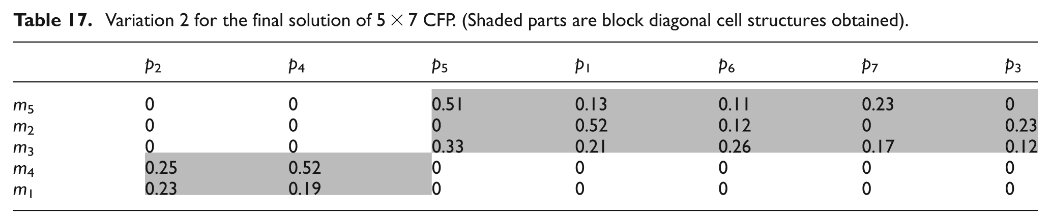
Variation 2 is obtained after small alteration done over solution matrix of Table 14. It is shown in Table 17, part 6 is no longer being process through machine 4 and machine 1 rather being processed through machine 2 and machine 5 and part 5 is being processed through machine 3 instead of being processed through machine 1. In this new configuration, the number of exceptional elements is 0 and number of voids is 3. The computed values of MGE and UGE are 87.54% and 85.76%, respectively.

Table 17.
Variation 2 for the final solution of 5 × 7 CFP. (Shaded parts are block diagonal cell structures obtained)

p ₂ p ₄ p ₅ p ₁ p ₆ p ₇ p ₃

m ₅ 0 0 0.51 0.13 0.11 0.23 0

m ₂ 0 0 0 0.52 0.12 0 0.23

m ₃ 0 0 0.33 0.21 0.26 0.17 0.12

m ₄ 0.25 0.52 0 0 0 0 0

m ₁ 0.23 0.19 0 0 0 0 0

Variation 3 is obtained after a small amount of changes in Table 14 (original solution) and shown in Table 18. Here, part 6 is no longer being process through machine 4 and machine 1 rather being processed through machine 2 and machine 5. In this new configuration, the number of exceptional elements is 1 and number of voids is 4. The computed values of MGE and UGE are 78.74% and 68.63%, respectively.

Table 18.
Variation 3 for the final solution of 5 × 7 CFP. (Shaded parts are block diagonal cell structures obtained)

p ₂ p ₄ p ₅ p ₁ p ₆ p ₇ p ₃

m ₅ 0 0 0.51 0.13 0.11 0.23 0

m ₂ 0 0 0 0.52 0.12 0 0.23

m ₃ 0 0 0 0.21 0.26 0.17 0.12

m ₄ 0.25 0.52 0 0 0 0 0

m ₁ 0.23 0.19 0.33 0 0 0 0

Variation 4 is the original solution matrix of Table 14 with three exceptional elements and six voids. The computed values of MGE and UGE are 70.25% and 53.45%, respectively.

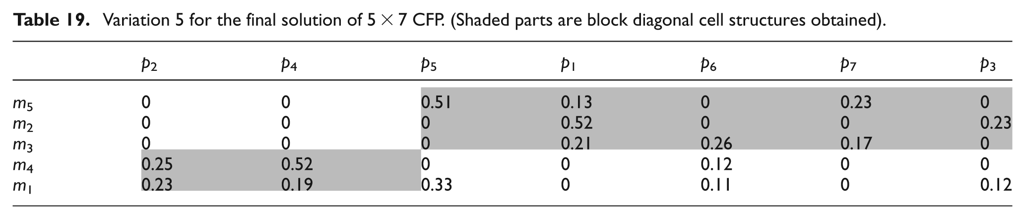
Variation 5 is portrayed in Table 19, where part 3 is no longer being processed through machine 3 rather being processed through machine 1. This configuration gives four exceptional elements and seven voids. The computed values of MGE and UGE are 66.54% and 46.56%, respectively.

Table 19.
Variation 5 for the final solution of 5 × 7 CFP. (Shaded parts are block diagonal cell structures obtained)

p ₂ p ₄ p ₅ p ₁ p ₆ p ₇ p ₃

m ₅ 0 0 0.51 0.13 0 0.23 0

m ₂ 0 0 0 0.52 0 0 0.23

m ₃ 0 0 0 0.21 0.26 0.17 0

m ₄ 0.25 0.52 0 0 0.12 0 0

m ₁ 0.23 0.19 0.33 0 0.11 0 0.12

This above analysis is briefed down in Table 20 for all the presented variations of cellular configurations.

Table 20.
Summary of sensitivity analysis.

Variations No. of voids and exceptional elements MGE UGE

1 Voids = 0; exceptional elements = 0 100 100

2 Voids = 3; exceptional elements = 0 87.54 85.76

3 Voids = 4; exceptional elements = 1 78.74 68.63

4 Voids = 6; exceptional elements = 3 70.25 53.45

5 Voids = 7; exceptional elements = 4 66.54 46.56

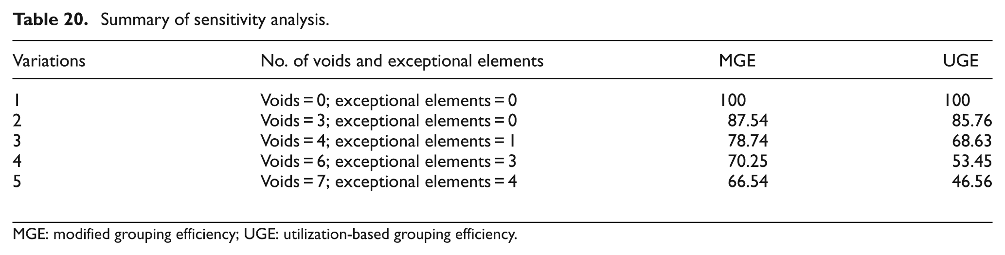
MGE: modified grouping efficiency; UGE: utilization-based grouping efficiency.

The above observations are plotted in Figure 8, which clearly portrays the sensitivity of UGE over MGE for small changes in the same solution. Addition or elimination of one void or exceptional element makes drastic change in the response of UGE. The changes are crisp and clear for UGE over MGE. For a large size and more scattered dataset, these small changes would be hard to visualize in MGE response curve. But due to the design features of UGE, these changes would be significantly prominent in UGE response curve. Therefore, the above analysis shows that the UGE is much sensitive than MGE when the dataset is a sparse matrix and changes in solution are small.

Figure 8.
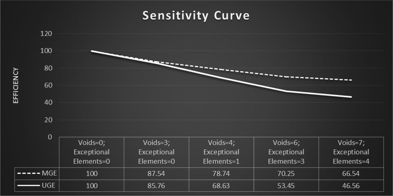
Sensitivity curve obtained from Table 20.

Qualitative analysis

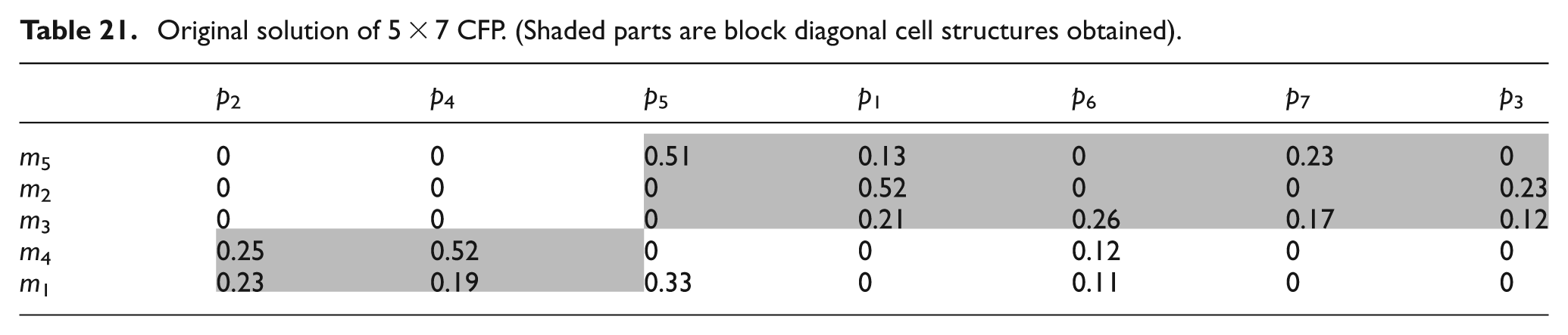
Measuring the solution quality realistically is an essential decisive factor of any performance measure in CMS. Most of the performance measures are solely focused on minimizing exceptional elements and voids.⁵⁸ However, this is not the sole objective of a good cellular configuration in practice. Since the CFP considered in this article is based on machine utilizations, the objective of a good cellular configuration is to minimize the TU of exceptional elements along with the number of exceptional elements and voids. To authenticate this observation, the original solution of Table 14 is considered and displayed in Table 21. This solution matrix produces three exceptional elements and six voids. The computed values of MGE and UGE are 70.25% and 53.45%, respectively.

Table 21.
Original solution of 5 × 7 CFP. (Shaded parts are block diagonal cell structures obtained)

p ₂ p ₄ p ₅ p ₁ p ₆ p ₇ p ₃

m ₅ 0 0 0.51 0.13 0 0.23 0

m ₂ 0 0 0 0.52 0 0 0.23

m ₃ 0 0 0 0.21 0.26 0.17 0.12

m ₄ 0.25 0.52 0 0 0.12 0 0

m ₁ 0.23 0.19 0.33 0 0.11 0 0

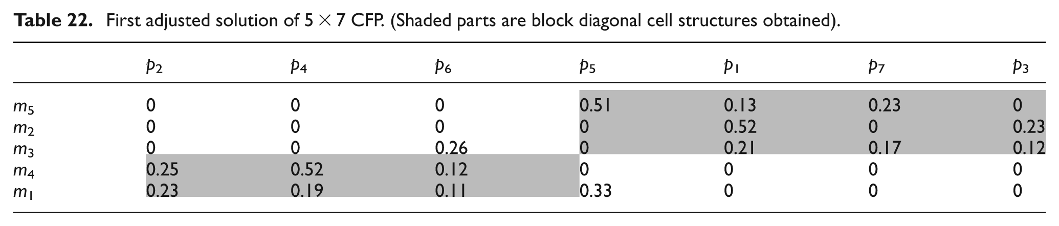
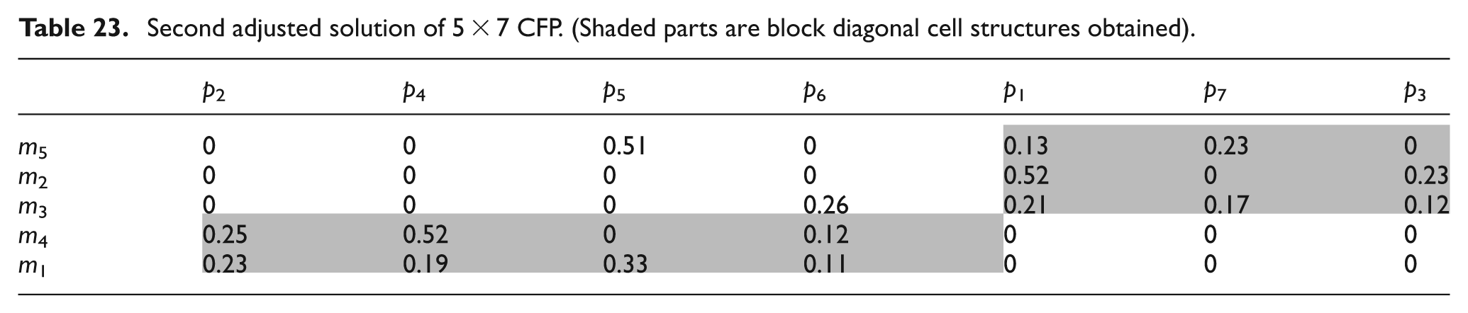
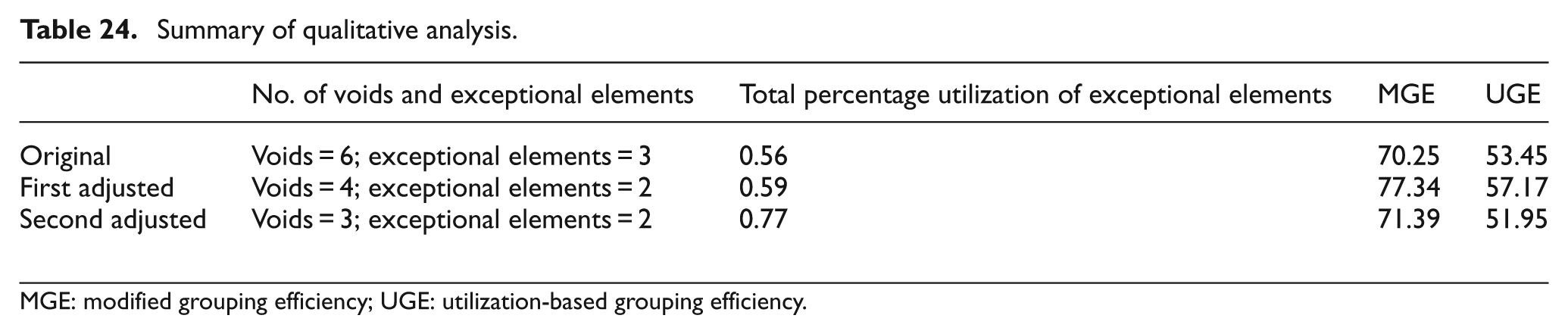
In the course of this analysis, this original solution matrix is altered in such a way that the number of exceptional elements and voids is minimized. Therefore, part 6 is moved to cell 1 from cell 2 in first adjusted solution (Table 22) and parts 5 and 6 both are transferred from cell 2 to cell 1 in second adjusted solution (Table 23). It is clearly visible that in the first adjusted solution matrix, the number of exceptional elements is 2 and the number of voids is 4, and for the second adjusted solution matrix, the number of exceptional elements is 2 and the number of voids is 3. Therefore, it can be presumed that the adjusted solutions are better than the original solution and performance measures are believed to attain a better efficiency value for these solutions. The computed values of MGE and UGE are shown in Table 24. This can be distinctly observed that the MGE caters an improved score for both the adjusted solutions while UGE obtains an inferior score for second adjusted solution but shows enhancement in first adjusted solution.

Table 22.
First adjusted solution of 5 × 7 CFP. (Shaded parts are block diagonal cell structures obtained)

p ₂ p ₄ p ₆ p ₅ p ₁ p ₇ p ₃

m ₅ 0 0 0 0.51 0.13 0.23 0

m ₂ 0 0 0 0 0.52 0 0.23

m ₃ 0 0 0.26 0 0.21 0.17 0.12

m ₄ 0.25 0.52 0.12 0 0 0 0

m ₁ 0.23 0.19 0.11 0.33 0 0 0

Table 23.
Second adjusted solution of 5 × 7 CFP. (Shaded parts are block diagonal cell structures obtained)

p ₂ p ₄ p ₅ p ₆ p ₁ p ₇ p ₃

m ₅ 0 0 0.51 0 0.13 0.23 0

m ₂ 0 0 0 0 0.52 0 0.23

m ₃ 0 0 0 0.26 0.21 0.17 0.12

m ₄ 0.25 0.52 0 0.12 0 0 0

m ₁ 0.23 0.19 0.33 0.11 0 0 0

Table 24.
Summary of qualitative analysis.

No. of voids and exceptional elements Total percentage utilization of exceptional elements MGE UGE

Original Voids = 6; exceptional elements = 3 0.56 70.25 53.45

First adjusted Voids = 4; exceptional elements = 2 0.59 77.34 57.17

Second adjusted Voids = 3; exceptional elements = 2 0.77 71.39 51.95

MGE: modified grouping efficiency; UGE: utilization-based grouping efficiency.

This observation illustrates a critical inference; MGE is capable of assessing the solution matrix in terms of number of exceptional elements and voids only but completely fails to realize the total percentage utilization outside of the block diagonal cellular structure. However, the proposed UGE not only focuses on the total percentage utilization of exceptional elements but also keeps track of the number exceptional elements and voids. Therefore, UGE can trade-off between these two issues and assist in achieving best solution so far. Hence, finally, the first adjusted solution can be called a more optimized solution in terms of the quality of solution after observing the behavior of UGE while MGE is incompetent for that matter.

It is concluded that the proposed UGE is shown to be much improved and relevant measure of efficiency for the CFP with “ratio data.” UGE not only improves its score with the reduced number of exceptional elements and void but also it is enhanced with the minimized value of the TU of the exceptional elements which is an important aspect in the real production situation. UGE is also shown to be much sensitive with the variation in data. Small amount of deviations in block diagonal cellular structure can change the UGE score drastically which would be more prominent for large-size sparse matrix.

Results and discussion

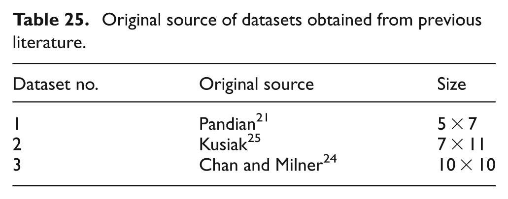
In section “Problem definitions,” it has been observed that obtaining appropriate test problems is one of the trickiest tasks of solving CFP in real time. Merely generating random matrices would be an incompetent method since condition 2 (equation (4)) could get violated. Therefore, this logic would negate the statement by Mahapatra and Pandian:²⁰“The real valued matrix is produced by assigning random numbers in the range of 0.5 to 1 as uniformly distributed values by replacing the ones in the incidence matrix and zeros to remain in its same positions” (p. 637). In reality, nearly all the past literature dealt with ratio data in CMS, overlooked condition 2 (equation (4)), which is an essential part while designing the datasets. Therefore, any of the existing datasets from past literature would not be an absolute choice for the CFP considered in this article. However, three existing datasets are considered from published articles which are small to medium in size and displayed in Table 25. All these datasets do not satisfy condition 2 (equation (4)). Hence, these three test problems are adjusted and condition 2 is imposed and made working for the model of CFP considered here.

Table 25.
Original source of datasets obtained from previous literature.

Dataset no. Original source Size

1 Pandian²¹ 5 × 7

2 Kusiak²⁵ 7 × 11

3 Chan and Milner²⁴ 10 × 10

The first adjusted dataset is the 5 × 7 test problem which is depicted in Table 2 and is also portrayed in Figure 9. Second and third adjusted datasets are displayed in Figures 10 and 11, respectively. The proposed MCDT model based on AHP is used to solve these test problems and obtained results are compared with McQueen’s⁵⁴ K-means algorithm successfully.

Figure 9.
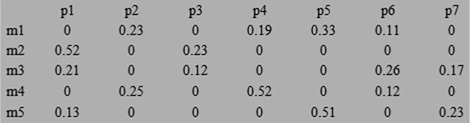
Redesigned dataset of King and Nakornchai²² (5 × 7).

Figure 10.
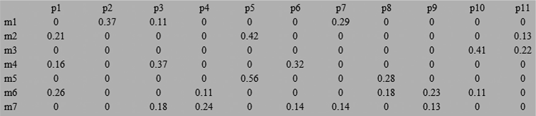
Redesigned dataset of Kusiak²⁵ (7 × 11).

Figure 11.
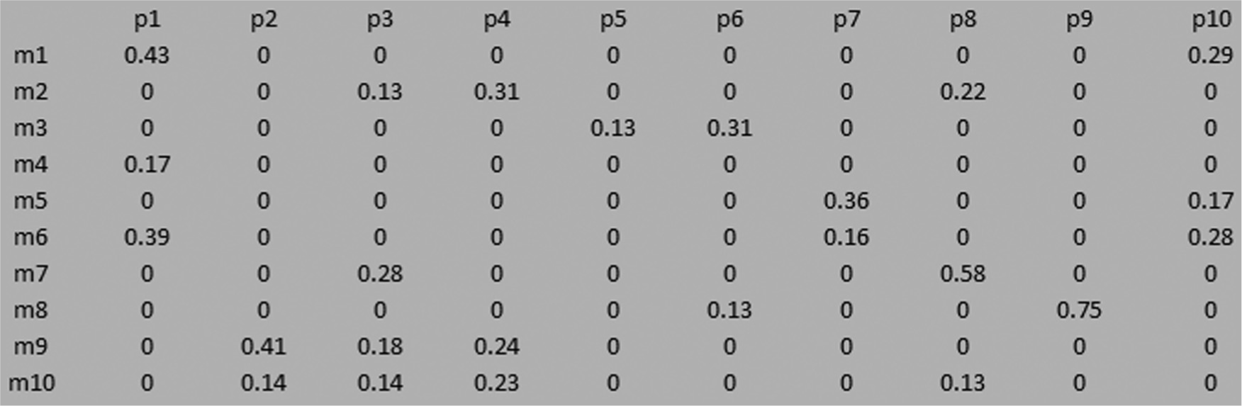
Redesigned dataset of Mosier and Taube²⁹ (10 × 11).

Both the techniques are coded in MATLAB 7.6 and tested on Intel Core i3 Processor with 4 GB RAM. The test problems in the form of matrices are the input to the K-means algorithm and the pairwise comparison matrices are the input to the MCDT model. Comparison results are depicted in Table 26, which demonstrate the competency of the proposed MCDT model based on AHP over K-means algorithm.

Table 26.
Result comparison among MCDT model and K-means method.

S. no. Size No. of cells MCDT model based on AHP
McQueen’s K-means

No. of voids and exceptional elements Total percentage utilization of exceptional elements UGE CPU time No. of voids and exceptional elements Total percentage utilization of exceptional elements UGE CPU time

1 5 × 7 2 Voids = 6; exceptional elements = 3 0.56 53.45 0.021 Voids = 3; exceptional elements = 2 0.77 51.95 0.045

2 7 × 11 3 Voids = 16; exceptional elements = 7 0.91 37.13 0.066 Voids = 14; exceptional elements = 7 1.4 31.70 0.113

3 10 × 10 3 Voids = 15; exceptional elements = 1 0.31 60.76 0.104 Voids = 17; exceptional elements = 7 1.26 33.35 0.143

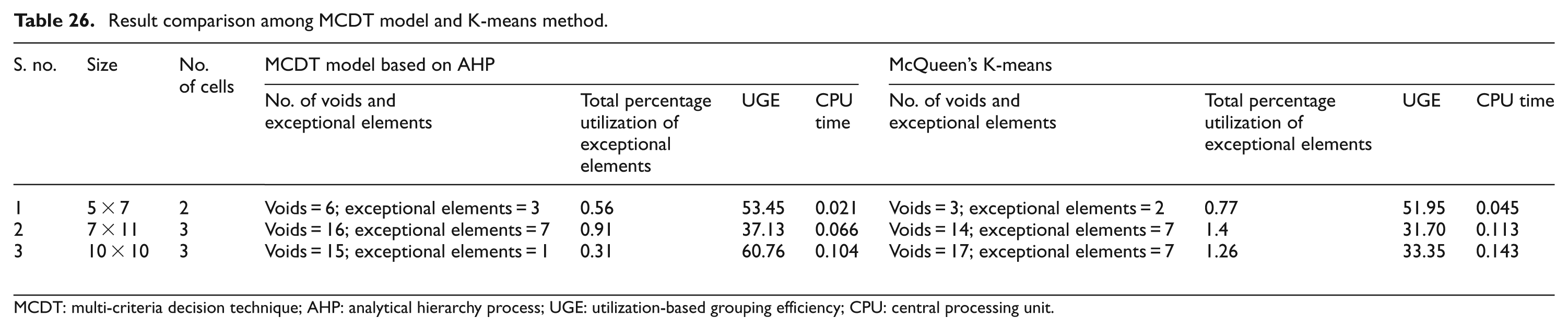
MCDT: multi-criteria decision technique; AHP: analytical hierarchy process; UGE: utilization-based grouping efficiency; CPU: central processing unit.

Table 26 shows that MCDT model has the ability to find good solutions for the CFPs. This novel technique not only reduces the exceptional elements and voids but also minimizes the total percentage utilization of exceptional elements and produces improved UGE scores for all the problem instances. This method clearly outperforms the K-means method which is a standing cell formation technique and used heavily in past literatures.^3,13,58 MCDT model is also slightly quicker than the K-means method in terms of CPU time. A graphical analysis on the performance of the proposed approach and the improvement in terms of CPU time is presented in Figure 12. All the solution matrices obtained by MCDT model and K-means method are portrayed in Figures 13 –18.

Figure 12.
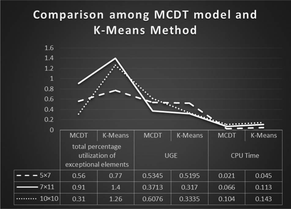
Graphical comparison among MCDT model and K-means methods.

Figure 13.
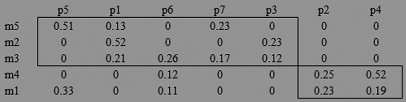
Solution of 5 × 7 CFP by MCDT model.

Figure 14.
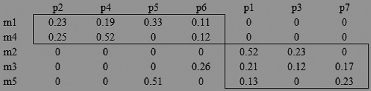
Solution of 5 × 7 CFP by K-means method.

Figure 15.
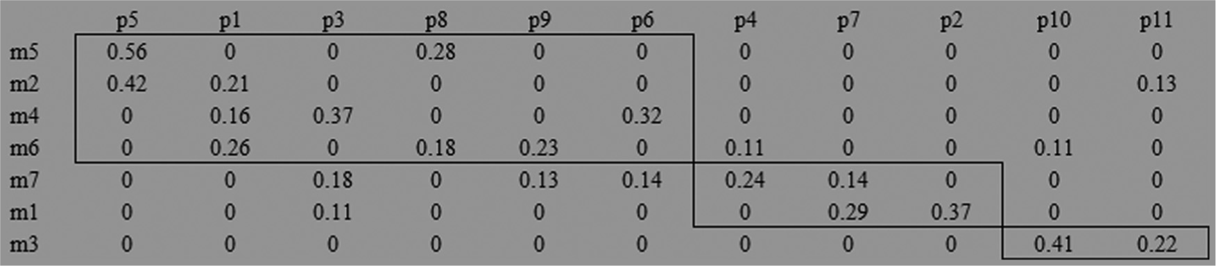
Solution of 7 × 11 CFP by MCDT model.

Figure 16.
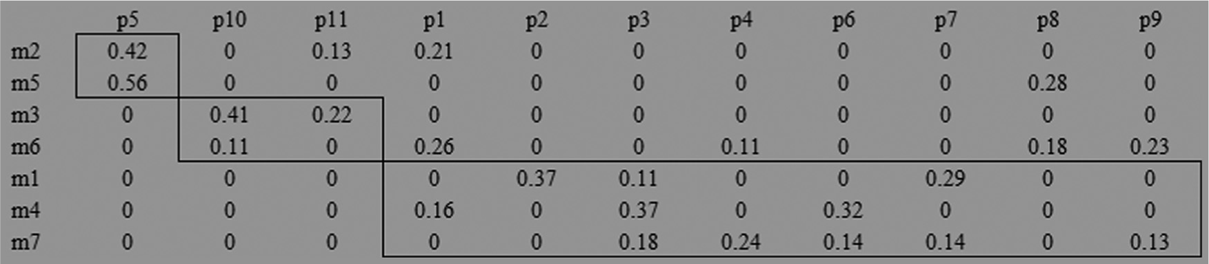
Solution of 7 × 11 CFP by K-means method.

Figure 17.
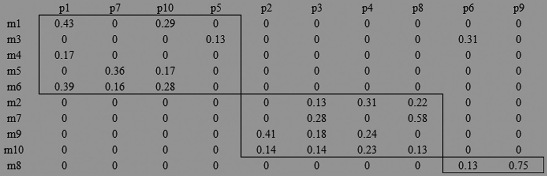
Solution of 10 × 10 CFP by MCDT model.

Figure 18.
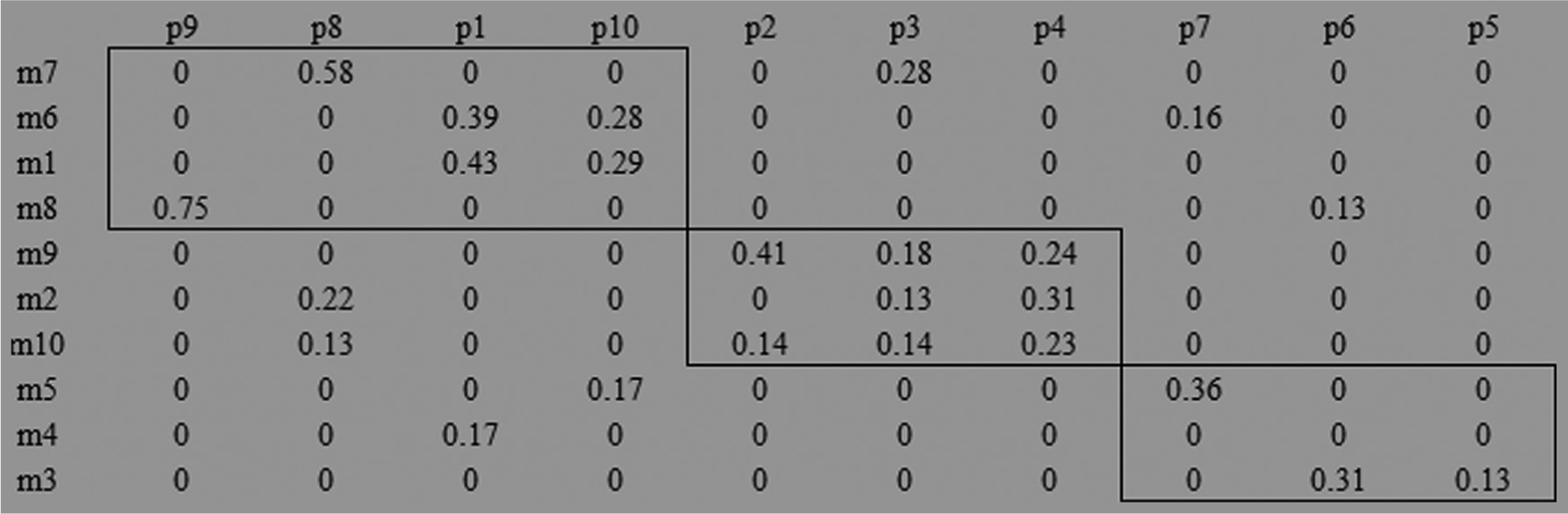
Solution of 10 × 10 CFP by K-means method.

Conclusion

This article is an attempt to put together three novel verdicts for the CFPs in CMS. First, it shows that the “ratio data” is in fact “percentage utilization of machines,” not “processing time.” Therefore, the intention of the researchers observed in past literature, to generate the “processing time”-based test problem with simple random function call, is incorrect. In order to rectify this, the datasets are adjusted scientifically. Thereafter, a novel AHP-based method is proposed as a cell formation technique which utilizes a modified Saaty’s scale which further exploits machine utilization phenomenon conveniently. This article shows that AHP method could be substantially handy while generating quick solutions to the CFPs. Finally, a novel grouping measure called UGE is proposed which is critically analyzed and compared with its nearest predecessor MGE. UGE is displayed to be substantially improved and relevant grouping measure for the “ratio data”-based CFPs. This field of study still has enormous possibilities to be explored. This research could be extended further in many directions such as development of a universal data generation algorithm for the problem considered, development of suitable similarity coefficient based on machine utilization factor, development of mathematical formulation of the problem to manage large datasets and implementation of the model in realistic production shop-floor.

	p ₁	p ₂	p ₃	p ₄	p ₅	p ₆	p ₇	Available machine hours
m ₁	0	7.4	0	3.9	6.5	2.1	0	2080
m ₂	7.7	0	4.6	0	0	0	0	2080
m ₃	3.1	0	2.4	0	0	4.9	5.1	2080
m ₄	0	8	0	10.8	0	2.3	0	2080
m ₅	1.9	0	0	0	10.1	0	6.8	2080
Volume	140	65	105	100	105	110	70

	p ₁	p ₂	p ₃	p ₄	p ₅	p ₆	p ₇	Total percentage utilization of machines
m ₁	0	0.23	0	0.19	0.33	0.11	0	0.86
m ₂	0.52	0	0.23	0	0	0	0	0.75
m ₃	0.21	0	0.12	0	0	0.26	0.17	0.76
m ₄	0	0.25	0	0.52	0	0.12	0	0.89
m ₅	0.13	0	0	0	0.51	0	0.23	0.87

Importance value	Definition	Description
1	Equal strong	Two factors are equally contributing to objective
3	Moderate strong	One factor is marginally superior over other
5	Fairly strong	One factor is strongly superior over other
7	Very strong	One factor is very strongly superior over other
9	Absolute strong	The highest level of superiority of one factor over other
2, 4, 6, 8	Intermediate values	According to the negotiation required

d_i_(i ₊ ₁₎ values	Saaty’s value	Definition
0–1	1	Equal strong
1–2.5	2	Intermediate values
2.5–3.5	3	Moderate strong
3.5–4.5	4	Intermediate values
4.5–5.5	5	Fairly strong
5.5–6.5	6	Intermediate values
6.5–7.5	7	Very strong
7.5–8.5	8	Intermediate values
8.5–rest	9	Absolute strong

	m ₁	m ₂	m ₃	m ₄	m ₅
Weights	0.245	0.05	0.054	0.36	0.291

	p ₁	p ₂	p ₃	p ₄	p ₅	p ₆	p ₇
Weights	0.048	0.381	0.046	0.179	0.207	0.094	0.048

	p ₁	p ₂	p ₃	p ₄	p ₅	p ₆	p ₇
Weights	0.552	0.048	0.209	0.048	0.048	0.048	0.048

	p ₁	p ₂	p ₃	p ₄	p ₅	p ₆	p ₇
Weights	0.234	0.058	0.122	0.058	0.058	0.3	0.17

	p ₁	p ₂	p ₃	p ₄	p ₅	p ₆	p ₇
Weights	0.045	0.204	0.046	0.536	0.048	0.081	0.046

	p ₁	p ₂	p ₃	p ₄	p ₅	p ₆	p ₇
Weights	0.132	0.526	0.04	0.04	0.226	0.068	0.154

	p ₁	p ₂	p ₃	p ₄	p ₅	p ₆	p ₇
m₁ (RW = 0.245)	0.048	0.381	0.046	0.179	0.207	0.094	0.048
m₂ (RW = 0.05)	0.552	0.048	0.209	0.048	0.048	0.048	0.048
m₃ (RW = 0.054)	0.234	0.058	0.122	0.058	0.058	0.3	0.17
m₄ (RW = 0.36)	0.045	0.204	0.046	0.536	0.048	0.081	0.046
m₅ (RW = 0.291)	0.132	0.526	0.04	0.04	0.226	0.068	0.154
Composite score	0.106 (4)	0.268 (1)	0.056 (7)	0.254 (2)	0.141 (3)	0.09 (5)	0.084 (6)

	m ₁	m ₂	m ₃	m ₄	m ₅
Composite score	0.127 (5)	0.258 (2)	0.196 (3)	0.139 (4)	0.28 (1)

	p ₂	p ₄	p ₅	p ₁	p ₆	p ₇	p ₃
m ₅	0	0	0.51	0.13	0	0.23	0
m ₂	0	0	0	0.52	0	0	0.23
m ₃	0	0	0	0.21	0.26	0.17	0.12
m ₄	0.25	0.52	0	0	0.12	0	0
m ₁	0.23	0.19	0.33	0	0.11	0	0

	p ₂	p ₄	p ₅	p ₁	p ₆	p ₇	p ₃
m ₅	0	0	0.51	0.13	0	0.23	0
m ₂	0	0	0	0.52	0	0	0.23
m ₃	0	0	0	0.21	0.26	0.17	0.12
m ₄	0.25	0.52	0	0	0.12	0	0
m ₁	0.23	0.19	0.33	0	0.11	0	0

Cells	1	2
Machines	m₂, m₃, m₅	p₁, p₃, p₅, p₆, p₇
Parts	m₁, m₄	p₂, p₄

	p ₂	p ₄	p ₅	p ₁	p ₆	p ₇	p ₃
m ₅	0	0	0.51	0.13	0.11	0.23	0.01
m ₂	0	0	0.11	0.52	0.12	0.02	0.23
m ₃	0	0	0.33	0.21	0.26	0.17	0.12
m ₄	0.25	0.52	0	0	0	0	0
m ₁	0.23	0.19	0	0	0	0	0

	p ₂	p ₄	p ₅	p ₁	p ₆	p ₇	p ₃
m ₅	0	0	0.51	0.13	0.11	0.23	0
m ₂	0	0	0	0.52	0.12	0	0.23
m ₃	0	0	0.33	0.21	0.26	0.17	0.12
m ₄	0.25	0.52	0	0	0	0	0
m ₁	0.23	0.19	0	0	0	0	0

	p ₂	p ₄	p ₅	p ₁	p ₆	p ₇	p ₃
m ₅	0	0	0.51	0.13	0.11	0.23	0
m ₂	0	0	0	0.52	0.12	0	0.23
m ₃	0	0	0	0.21	0.26	0.17	0.12
m ₄	0.25	0.52	0	0	0	0	0
m ₁	0.23	0.19	0.33	0	0	0	0

	p ₂	p ₄	p ₅	p ₁	p ₆	p ₇	p ₃
m ₅	0	0	0.51	0.13	0	0.23	0
m ₂	0	0	0	0.52	0	0	0.23
m ₃	0	0	0	0.21	0.26	0.17	0
m ₄	0.25	0.52	0	0	0.12	0	0
m ₁	0.23	0.19	0.33	0	0.11	0	0.12

Variations	No. of voids and exceptional elements	MGE	UGE
1	Voids = 0; exceptional elements = 0	100	100
2	Voids = 3; exceptional elements = 0	87.54	85.76
3	Voids = 4; exceptional elements = 1	78.74	68.63
4	Voids = 6; exceptional elements = 3	70.25	53.45
5	Voids = 7; exceptional elements = 4	66.54	46.56

	p ₂	p ₄	p ₅	p ₁	p ₆	p ₇	p ₃
m ₅	0	0	0.51	0.13	0	0.23	0
m ₂	0	0	0	0.52	0	0	0.23
m ₃	0	0	0	0.21	0.26	0.17	0.12
m ₄	0.25	0.52	0	0	0.12	0	0
m ₁	0.23	0.19	0.33	0	0.11	0	0

	p ₂	p ₄	p ₆	p ₅	p ₁	p ₇	p ₃
m ₅	0	0	0	0.51	0.13	0.23	0
m ₂	0	0	0	0	0.52	0	0.23
m ₃	0	0	0.26	0	0.21	0.17	0.12
m ₄	0.25	0.52	0.12	0	0	0	0
m ₁	0.23	0.19	0.11	0.33	0	0	0

	p ₂	p ₄	p ₅	p ₆	p ₁	p ₇	p ₃
m ₅	0	0	0.51	0	0.13	0.23	0
m ₂	0	0	0	0	0.52	0	0.23
m ₃	0	0	0	0.26	0.21	0.17	0.12
m ₄	0.25	0.52	0	0.12	0	0	0
m ₁	0.23	0.19	0.33	0.11	0	0	0

	No. of voids and exceptional elements	Total percentage utilization of exceptional elements	MGE	UGE
Original	Voids = 6; exceptional elements = 3	0.56	70.25	53.45
First adjusted	Voids = 4; exceptional elements = 2	0.59	77.34	57.17
Second adjusted	Voids = 3; exceptional elements = 2	0.77	71.39	51.95

Dataset no.	Original source	Size
1	Pandian²¹	5 × 7
2	Kusiak²⁵	7 × 11
3	Chan and Milner²⁴	10 × 10

S. no.	Size	No. of cells	MCDT model based on AHP	McQueen’s K-means
1	5 × 7	2	Voids = 6; exceptional elements = 3	0.56	53.45	0.021	Voids = 3; exceptional elements = 2	0.77	51.95	0.045
2	7 × 11	3	Voids = 16; exceptional elements = 7	0.91	37.13	0.066	Voids = 14; exceptional elements = 7	1.4	31.70	0.113
3	10 × 10	3	Voids = 15; exceptional elements = 1	0.31	60.76	0.104	Voids = 17; exceptional elements = 7	1.26	33.35	0.143

Footnotes

Declaration of conflicting interests

The author(s) declared no potential conflicts of interest with respect to the research, authorship and/or publication of this article.

Funding

The author Tamal Ghosh (IF120670) is thankful to DST-INSPIRE governing body of Department of Science & Technology, Government of India, for the financial support to carry out the doctoral research.

References

Won

Currie

. Fuzzy ART/RRR-RSS: a two-phase neural network algorithm for part-machine grouping in cellular manufacturing. Int J Prod Res 2007; 45(9): 2073–2104.

Selim

Askin

Vakharia

. Cell formation in group technology: review evaluation and directions for future research. Comput Ind Eng 1998; 34(1): 3–20.

Venugopal

Narendran

. Cell formation in manufacturing systems through simulated annealing: an experimental evaluation. Eur J Oper Res 1992; 63: 409–422.

McCormick

Schweitzer

JPJ

White

. Problem decomposition and data reorganization by a clustering technique. Oper Res 1972; 20(5): 993–1009.

Rajagopalan

Batra

. Design of cellular production system—a graph theoretic approach. Int J Prod Res 1975; 13(6): 567–579.

King

. Machine-component grouping in production flow analysis: an approach using a rank order-clustering algorithm. Int J Prod Res 1980; 18: 213–232.

Chandrasekharan

Rajagopalan

. MODROC: an extension of rank order clustering for group technology. Int J Prod Res 1986; 24(5): 1221–1233.

Srinivasan

. A clustering algorithm for machine cell formation in group technology using minimum spanning trees. Int J Prod Res 1994; 32(9): 2149–2158.

Dimopoulos

Mort

. A hierarchical clustering methodology based on genetic programming for the solution of simple cell-formation problems. Int J Prod Res 2001; 39(1): 1–19.

10.

Xambre

Vilarinho

. A simulated annealing approach for manufacturing cell formation with multiple identical machines. Eur J Oper Res 2003; 151: 434–446.

11.

Durán

Rodriguez

Consalter

. A PSO-based clustering algorithm for manufacturing cell design. In: Workshop on knowledge discovery and data mining, Adelaide, SA, Australia, 23–24 January 2008, pp.72–75. New York: IEEE.

12.

Sayadi

Hafezalkotob

Naini

SGJ

. Firefly-inspired algorithm for discrete optimization problems: an application to manufacturing cell formation. J Manuf Syst 2013; 32(1): 78–84.

13.

Sengupta

Ghosh

Dan

. Fuzzy ART K-Means Clustering Technique (FAKMCT)—a hybrid neural network approach to cellular manufacturing systems. Int J Comput Integ M 2011; 24(10): 927–938.

14.

Satheeshkumar

Karthikeyan

Renald

CJT

. Evaluation of cell formation algorithms and implementation of MOD-SLC algorithm as an effective cellular manufacturing system in a manufacturing industry. Int J Curr Eng Technol. Epub ahead of print 2014. DOI: 10.14741/ijcet/spl.2.2014.33.

15.

Nair

Narendran

. ACCORD: a bicriterion algorithm for cell formation using ordinal and ratio level data. Int J Prod Res 1999; 37(3): 539–556.

16.

Kumar

Jain

. Part-machine group formation with ordinal-ratio level data and production volume. Int J Simulat Model 2009; 8(2): 90–101.

17.

Chattopadhyay

Dan

Mazumdar

. Application of visual clustering properties of self-organizing map in machine-part cell formation. Appl Soft Comput 2012; 12(2): 600–610.

18.

Lee

Ahn

. GT efficacy: a performance measure for cell formation with sequence data. Int J Prod Res 2013; 51(20): 6070–6081.

19.

George

Rajendran

Ghosh

. An analytical-iterative clustering algorithm for cell formation in cellular manufacturing systems with ordinal-level and ratio-level data. Int J Adv Manuf Tech 2003; 2: 125–133.

20.

Mahapatra

Pandian

. Genetic cell formation using ratio level data in cellular manufacturing systems. Int J Adv Manuf Tech 2008; 38: 630–640.

21.

Pandian

. Application of soft computing techniques for cell formation considering operational for cell formation considering operational time and sequence. PhD Thesis, NIT Rourkela, Rourkela, India, 2008.

22.

King

Nakornchai

. Machine-component group formation in group technology: review and extension. Int J Prod Res 1982; 20: 117–133.

23.

Waghodekar

Sahu

. Machine-component cell formation in group technology: MACE. Int J Prod Res 1984; 22(6): 937–948.

24.

Chan

Milner

. Direct clustering algorithm for group formation in cellular manufacturing. J Manuf Syst 1982; 1: 65–75.

25.

Kusiak

. The generalized group technology concept. Int J Prod Res 1987; 25(4): 561–569.

26.

Srinivasan

Narendran

. GRAFICS: a non-hierarchical clustering algorithm for group technology. Int J Prod Res 1991; 29(3): 463–478.

27.

Seifoddini

. Duplication process in machine cells formation in group technology. IIE Trans 1989; 21(4): 382–388.

28.

Shafer

Rogers

. Similarity and distance measures for cellular manufacturing. Int J Prod Res 1993; 31(5): 1131–1142.

29.

Mosier

Taube

. Weighted similarity measure heuristics for the group technology machine clustering problem. Omega 1985; 13(6): 577–583.

30.

McAuley

. Machine grouping for efficient production. Prod Engineer 1972; 51(2): 53–57.

31.

Prabhakaran

Janakiraman

Sachithanandam

. Manufacturing data based combined dissimilarity coefficient for machine cell formation. Int J Adv Manuf Tech 2002; 19: 889–897.

32.

Seifoddini

Wolfe

. Application of the similarity coefficient method in group technology. IIE Trans 1986; 183: 271–277.

33.

Ballakur

Steudel

. A with-in cell utilization based heuristic for designing cellular manufacturing systems. Int J Prod Res 1987; 25(5): 639–655.

34.

Veeramani

Mani

. A polynomial-time algorithm for optimal clustering in a special class of {0, 1}-matrices. Int J Prod Res 1996; 34(9): 2587–2611.

35.

Rabbani

Samavati

Ziaee

. Reconfigurable dynamic cellular manufacturing system: a new bi-objective mathematical model. RAIRO: Oper Res 2014; 48: 75–102.

36.

Boctor

. A linear formulation of the machine-part cell formation problem. Int J Prod Res 1991; 29(2): 343–356.

37.

Ramabhatta

Nagi

. Integrated formulation of manufacturing cell formation with capacity planning and multiple routings. Ann Oper Res 1998; 77: 79–95.

38.

Logendran

Ramakrishna

. Manufacturing cell formation in the presence of lot splitting and multiple units of same machine. Int J Prod Res 1995; 33: 675–693.

39.

Adenso-Diaz

Lozano

Racero

. Machine cell formation in generalized group technology. Comput Ind Eng 2001; 41: 227–240.

40.

Dagli

Huggahalli

. Neural network approach to group technology. In: Wang

Takefuji

(eds) Neural networks in design and manufacturing. Singapore: World Scientific Publishing Company, 1993, pp.1–55.

41.

Kao

Moon

. A unified group technology implementation using the backpropagation learning rule of neural networks. Comput Ind Eng 1991; 20(4): 425–437.

42.

Kamal

Burke

. FACT: a new neural network based clustering algorithm for group technology. Int J Prod Res 1996; 34(4): 919–946.

43.

Gupta

Kumar

. A genetic algorithm-based approach to cell composition and layout design problems. Int J Prod Res 1996; 34(2): 447–482.

44.

Zolfaghari

Liang

. A new genetic algorithm for the machine/part grouping problem involving processing times and lot sizes. Comput Ind Eng 2003; 45: 713–731.

45.

Pillai

Subbarao

. A robust cellular manufacturing system design for dynamic part population using a genetic algorithm. Int J Prod Res 2008; 46(18): 5191–5210.

46.

Arkat

Hosseini

Farahani

. Minimization of exceptional elements and voids in the cell formation problem using a multi-objective genetic algorithm. Expert Syst Appl 2011; 38(8): 9597–9602.

47.

Khaksar-Haghani

Kia

Mahdavi

. A genetic algorithm for solving a multi-floor layout design model of a cellular manufacturing system with alternative process routings and flexible configuration. Int J Adv Manuf Tech 2013; 66: 845–865.

48.

Fan

Feng

. Design of cellular manufacturing system with quasi-dynamic dual resource using multi-objective GA. Int J Prod Res 2013; 51(14): 4134–4154.

49.

Bagheri

Bashiri

. A hybrid genetic and imperialist competitive algorithm approach to dynamic cellular manufacturing system. Proc IMechE, Part B: J Engineering Manufacture 2014; 228(3): 458–470.

50.

Chen

Cotruvo

Baek

. A simulated annealing solution to the cell formation problem. Int J Prod Res 1995; 33: 2601–2614.

51.

Zolfaghari

Liang

. Comparative study of simulated annealing, genetic algorithms and tabu search for solving binary and comprehensive machine-grouping problems. Int J Prod Res 2002; 40(9): 2141–2158.

52.

Spiliopoulos

Sofianopoulou

. An efficient ant colony optimisation system for the manufacturing cells formation system. Int J Adv Manuf Tech 2008; 36: 589–597.

53.

Nouri

Hong

. Development of bacteria foraging optimization algorithm for cell formation in cellular manufacturing system considering cell load variations. J Manuf Syst 2013; 32(1): 20–31.

54.

McQueen

. Some methods for classification and analysis of multivariate observations. In: Proceedings of Fifth symposium on mathematical statistics and probability, Berkeley, CA, 1967, (Univ. of Calif. Press) vol. 1: 281–297.

55.

Saaty

. The analytic hierarchy process: planning, priority setting, resource allocation. New York: McGraw-Hill, 1980.

56.

Ghosh

Chakraborty

Dan

. An effective AHP-based metaheuristic approach to solve supplier selection problem. Int J Procure Manag 2012; 5(2): 140–159.

57.

Kumar

Chandrasekharan

. Grouping efficacy: a quantitative criterion for goodness of block diagonal forms of binary matrices in group technology. Int J Prod Res 1990; 28: 2233–2243.

58.

Ponnambalam

Pandian

Mahapatra

. Cell formation with workload data in cellular manufacturing system using genetic algorithm. In: IEEE international conference on industrial engineering and engineering management, Singapore, 2–4 December 2007, pp.674–678. New York: IEEE.

59.

Sarkar

Khan

. A comparison of existing grouping efficiency measures and a new weighted grouping efficiency measure. IIE Trans 2001; 33: 11–27.

Utilization-based grouping efficiency and multi-criteria decision approach in designing of manufacturing cells

Abstract

Keywords

Introduction

Problem definitions

Condition 1

Condition 2

Problem instance

AHP-based algorithm

Step 1

Step 2

Step 2.1

Step 2.2

Step 2.3

Step 3

Step 3.1

Step 3.2

Step 4

Machine ranking method

Finalizing the cell formation solution

Performance measure

Sensitivity analysis

Qualitative analysis

Results and discussion

Conclusion

Footnotes

Declaration of conflicting interests

Funding

References