Sage Journals: Discover world-class research

Abstract

Manufacturing systems involve a huge number of combinatorial problems that must be optimized in an efficient way. One of these problems is related to task scheduling problems. These problems are NP-hard, so most of the complete techniques are not able to obtain an optimal solution in an efficient way. Furthermore, most of real manufacturing problems are dynamic, so the main objective is not only to obtain an optimized solution in terms of makespan, tardiness, and so on but also to obtain a solution able to absorb minor incidences/disruptions presented in any daily process. Most of these industries are also focused on improving the energy efficiency of their industrial processes. In this article, we propose a knowledge-based model to analyse previous incidences occurred in the machines with the aim of modelling the problem to obtain robust and energy-aware solutions. The resultant model (called dual model) will protect the more dynamic and disrupted tasks by assigning buffer times. These buffers will be used to absorb incidences during execution and to reduce the machine rate to minimize energy consumption. This model is solved by a memetic algorithm which combines a genetic algorithm with a local search to obtain robust and energy-aware solutions able to absorb further disruptions. The proposed dual model has been proven to be efficient in terms of energy consumption, robustness and stability in different and well-known benchmarks.

Keywords

Scheduling problem energy efficiency robustness dual model

Introduction

Nowadays, many companies and enterprises are focused on improving their benefits to be more competitive in their manufacturing processes. However, there exist other objectives beyond the benefits, such as robustness and sustainability. Manufacturing processes have a huge impact on the environment. Some of them such as chemical, food, refining, paint, or metal industries are highly energy consuming and present a high risk of producing an important amount of waste or pollution. For example, during 2000, about 60% of the US$700 million energy expenditures in 37 US automotive assembly plants are spent in painting processes.¹ In such a context, a 5% reduction in energy consumption may result in a saving of more than half million dollars per year for each plant. Industrial processes are also known to be the major sources of greenhouse gas (GHG) emissions. Statistics has shown that the GHG emitted from the usage of energy sources such as electricity, coal, oil and gas during manufacturing accounts for more than 37% even 50% of the world total GHG.²

Therefore, the enterprises have started to take steps to reduce GHG emission from their products and services under the mounting pressure stemming from the implementation of the Kyoto Protocol and Copenhagen Accord. Industrial sector has a lot of influence in the environmental impacts, because it represents the sector where more energy is used. The energy consumed in the world in 2011 was 524 quadrillion BTU (British thermal unit) and the energy used by the industrial sector amounts to 51%.³ So reducing consumption in this sector directly affects the total consumption. Nevertheless, it is still difficult for enterprises to consider renewable sources application and emissions reduction when making manufacturing and operation decisions, especially on the production planning and scheduling problems.⁴

During the last few years, many works have been carried out to optimize energy consumption in manufacturing processes based on the machine level and the product level.⁵ Besides, from the manufacturing system-level perspective, optimizing the objectives of production scheduling is a feasible and efficient approach for manufacturing companies to decrease energy consumption without any machine or product redesign. Recently, interesting efforts have been performed to investigate production-scheduling problems that take into account energy efficiency.

May et al.⁶ addressed a multi-objective scheduling model related to energy consumption and makespan in a job-shop system and obtained a series of different Pareto front solutions based on a green genetic algorithm (GA). Escamilla et al.⁷ developed a GA to minimize energy consumption and makespan in an extended version of the job-shop scheduling problem (JSP), where each machine can work at different rates. Mingcheng et al.⁸ built a multi-objective optimization (MOO) model involving makespan, processing cost, processing quality and energy consumption for a flexible JSP and designed a modified on-dominant sorting GA to solve it. Liu et al.⁹ established a scheduling model that minimized the total non-processing electricity consumption and total weighted tardiness for the JSP. This problem was solved by using a non-dominant sorting GA.

In the literature on dynamic scheduling problems, predictive–reactive scheduling strategies have been widely used in manufacturing systems, where schedules are revised in response to dynamic factors.¹⁰ Most of them consider only efficiency of the schedule like makespan. However, reducing energy consumption in production scheduling considering dynamic factors has been rather limited. Pach et al.¹¹ proposed a reactive scheduling model based on potential fields in flexible manufacturing systems, which considered three indicators: makespan, energy consumption and the number of resource switches in a dynamic context. Zheng et al.¹² proposed a dynamic shop floor rescheduling approach inspired by a neuroendocrine regulation mechanism.

The JSP represents a problem in which some tasks are assigned to machines with a specific processing time. We work with an extension of JSP where each machine can work at different rates, so each machine has different available processing times and energy consumptions. Thus, if a machine works at higher rate, it consumes more energy but the processing time is reduced. Energy efficiency is a critical parameter to take into account, but also other parameters such as robustness can result in schedule profitability, safety, or simplicity to avoid rescheduling, so robustness and energy efficiency can be considered in many real-life manufacturing problems.

Problem description

Many industrial processes can be represented as a JSP where machines can work at different speeds/rates (JSMS). This problem consists of a set of n jobs ${J_{1}, \dots, J_{n}}$ and a set of m machines ${R_{1}, \dots, R_{m}}$ . Each job $J_{i}$ consists of a sequence of $v_{i}$ tasks $(θ_{i 1}, \dots, θ_{i v_{i}})$ . Each task $θ_{il}$ has a single machine requirement $R_{θ_{il}}$ and a start time $s t_{θ_{il}}$ to be determined. Each machine can work at different rates, so different processing times and energy consumptions can be applied to each task.

A feasible schedule is composed of a complete assignment of starting times to tasks that satisfies the following constraints:

The tasks of each job are sequentially scheduled.

Each machine can process at most one task at any time.

No preemption is allowed.

The aim of the JSMS problems is to find a feasible schedule that minimizes makespan and energy consumption meanwhile maximizes the robustness of the schedule.

This problem represents an extension of the standard JSP $(J | | C_{\max})$ .¹³ The association between duration and energy has been created so the JSMS problem can be denoted as $J (Speed) | | C_{\max}, Energy$ . For each task, three different speeds have been defined to the involved machines. Each speed of the machine has been associated with a duration and an energy consumption. When the working speed of a machine increases, the energy consumption also increases, but the duration of the involved task decreases.

Robustness and stability

Robustness can be related with many real-world problems. In industry, robustness can be profitable, because if a perturbation appears in the schedule, it remains valid so it is not necessary to reschedule and, therefore, to interrupt the production process. We consider that a system is robust, if it is able to maintain its functionality even though some incidences can appear. In scheduling problems, a solution is robust if it is able to absorb some disruptions without the delay of further tasks.

In real world, problems are very common to leave some gaps/buffers between consecutive tasks of the schedule. Sometimes new gaps appear to satisfy precedence constraints. In JSMS problem, there is the possibility to change the speed of the machines, so increasing the speed of a machine can be enough to recover the incidences (energy-efficient buffer).

In JSMS problem, a solution (S) is robust if given an incidence (I); it only affects to one task, and it is able to be absorbed. In this case, the incidence can be absorbed by an existing gap, or the machine that executes this task can increase the speed to absorb the incidence. Moreover, a gap and an energy-efficient buffer can be joined to absorb incidences. If there is no buffer or it is smaller than the incidence size, the delay of a task is propagated to other tasks, so the solution is not considered robust. Thus, the robustness of a solution can be modelled as:

$R_{S, I} = 1$ , if only the affected task is modified by I. Thus a gap/buffer assigned to this task can absorb the incidence, or the machine can increase its speed to absorb the incidence.

$R_{S, I} = 0$ , if more tasks are affected by I. This means that the buffer assigned to this task cannot absorb the incidence and it is propagated to the rest of the schedule.

Thus, a robust solution is a solution that maintains its feasibility over the whole set of expected incidences. If a solution is not robust against a perturbation, it can be considered stable only when it is able to remain valid against incidences with only few changes.¹⁴ Thus, stability is an interest parameter for rescheduling in order to recover the original solution by means of modifying the value of only a few tasks.

Thus, we consider a solution S is $s - stable$ if there is a solution $S'$ , such that $| | S' - S | | < s$ , $where | | . | |$ is some n-dimensional norm defined in the solution space to evaluate the difference between S and $S'$ .¹⁵ So in our case, the difference between S and $S'$ can be the number of tasks that have to be changed to maintain feasibility.

Memetic algorithm (GA* + LS)

In this section, we present a memetic algorithm which combines a GA with a local search (LS). GAs are adaptive methods which may be used to solve optimization problems.¹⁶ They are based on the genetic process of biological organisms. Over many generations, natural populations evolve according to the principle of natural selection. At each generation, every new individual (chromosome) corresponds to a solution, that is, a schedule for the given JSMS instance. Before a GA can be run, a suitable encoding (representation) of the problem must be devised. The essence of a GA is to encode a set of parameters (known as genes) and to join them together to form a string of values (chromosome). A fitness function is also required, which assigns a figure of merit to each encoded solution. The fitness of an individual depends on its chromosome and is evaluated by the fitness function. During the run, parents must be selected for reproduction and recombined to generate offspring. Parents are randomly selected from the population, using a scheme which favours fitter individuals. Having selected two parents, their chromosomes are combined, typically by using crossover and mutation mechanisms to generate better offspring, so they represent better solutions. The process is iterated until a stopping criterion is satisfied.

Chromosome encoding and decoding

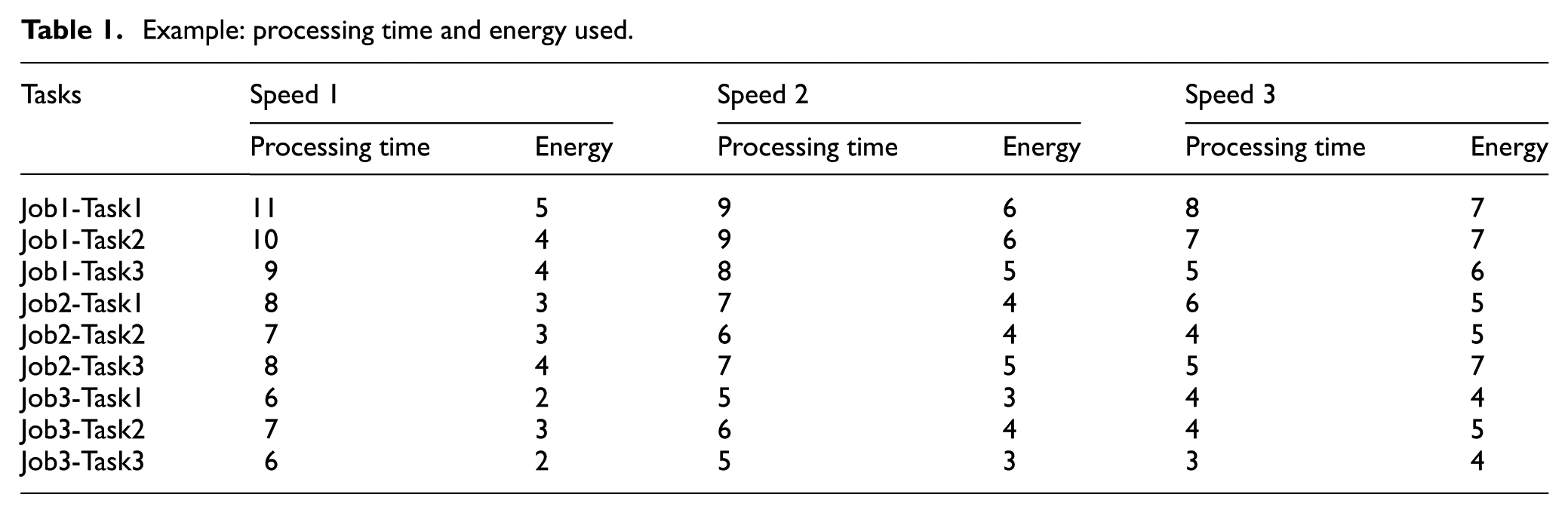
In GAs, each candidate represents a solution in the solution space. The first step to construct a GA is to define an appropriate genetic representation (coding). Table 1 shows an example of the processing time and the energy consumption of a JSMS composed of three jobs, three machines and three tasks per job. A chromosome is a permutation of the set of tasks that represents a tentative ordering to schedule them. The sequence (2 1 1 3 2 3 1 2 3) is a valid chromosome for this example, where each number of the sequence represents the job of the task. The first number ‘2’ represents the first task of the job 2 and it will be executed as soon as possible following the problem constraints. As it was shown in Varela et al.,¹⁷ this encoding has a number of interesting properties for the classic JSP. However, in the JSMS problem, the machine speed of each operation has to be represented. Thus, it is added a value to each task in order to represent the speed of the machine that processes this task. For instance, a valid chromosome could be (2 1 1 2 1 3 3 3 2 2 3 2 1 2 2 3 3 3) for the former example.⁷ The speed of each task is showed using underlined numbers. When the chromosome representation is decoded, each task starts as soon as possible following the precedence and machine constraints. With the machine speed representation, the processing time of each task and the energy consumption of the machine can be calculated. The decoding result is shown in Figure 5.

Table 1.

Example: processing time and energy used.

Tasks	Speed 1		Speed 2		Speed 3
Tasks	Processing time	Energy	Processing time	Energy	Processing time	Energy
Job1-Task1	11	5	9	6	8	7
Job1-Task2	10	4	9	6	7	7
Job1-Task3	9	4	8	5	5	6
Job2-Task1	8	3	7	4	6	5
Job2-Task2	7	3	6	4	4	5
Job2-Task3	8	4	7	5	5	7
Job3-Task1	6	2	5	3	4	4
Job3-Task2	7	3	6	4	4	5
Job3-Task3	6	2	5	3	3	4

Initial population and fitness

Each gene represents one task of the problem. The position of each task determines its dispatch order in this genome/solution. The initial chromosomes are obtained following some dispatching rules or by random permutation. We employ six common dispatching rules: shortest processing time (SPT), longest processing time (LPT), job with more load (JML), job with more tasks (JMT), machine with more load (MML) and machine with more tasks (MMT). We also employ a random rule, which select a job randomly from the remaining jobs. The dispatching rule SPT assigns high priority to short tasks, LPT assigns high priority to long tasks, JML assigns high priority to tasks which job has more load, JMT assigns high priority to tasks which job has more tasks, MML assigns high priority to tasks whose machine has more load and MMT assigns high priority to tasks whose machine has more tasks. To create each genome, each dispatching rule can be randomly selected with a probability of 10% and random rule with a probability of 40%. Thus, it obtains variety and diversity in the initial population in order to obtain good solutions. Each dispatching rule assigns a priority to each task. This priority can be based on attributes of the jobs, the machines, or tasks. The machine speed for each gene is generated depending on the value of $λ$ . For $λ$ values lower than 0.6 the machine speed value is set to 1; if $λ$ is higher than 0.6 the machine speed value is set to 2 or 3.

In a single objective optimization, there is a single optimal solution. However, in MOO not only one optimal solution but a set of optimal solutions can be identified. This set of optimal solutions composes the Pareto front. Diverse techniques have been developed to solve MOO problems. One of the most well-known methods for solving MOO problems is the normalized weighted additive utility function (NWAUF), where multiple objectives are normalized and added to form a utility function. NWAUF has been implemented in a wide range of MOO applications due to its simplicity and natural ability to identify efficient solutions. Let $f_{i}$ be the ith objective function value. Then, the NWAUF is defined as

U_{j} = w_{1} {f'}_{1} + w_{2} {f'}_{2} + \dots + w_{k} {f'}_{k}

(1)

where $w_{1}, w_{2}, \dots, w_{k}$ are weights of importance and ${f'}_{1}, {f'}_{2}, \dots, {f'}_{k}$ are normalized values of $f_{1}, f_{2}, \dots, f_{k}$ . By normalizing different objectives, all objectives are evaluated in the same scale. Weights show decision maker’s preference for each objective where, $\sum_{i = 1}^{k} w_{i} = 1$ ; $0 \leq w_{i} \leq 1$ for $i = 1, \dots, k$ . Using this utility function, the MOOs can now be solved as a single objective optimization problem.

The definition of fitness function is just the reciprocal of the objective function value. The objective is to find a solution that minimizes the multi-objective makespan and energy consumption. Following NWAUF rules, the fitness function (2) is created, where the weights assigned to both variables are given by the $λ$ value. Since the values of energy consumption and makespan are not proportional, it is necessary to normalize both measures. Makespan is divided by MaxMakespan which is the maximum makespan value in a GA execution when $λ = 0$ . MaxEnergy is the sum of the energy needed to execute all tasks at top speed

F = (λ * \frac{Makespan}{MaxMakespan} + (1 - λ) * \frac{SumEnergy}{MaxEnergy}) * 100

(2)

Crossover operator

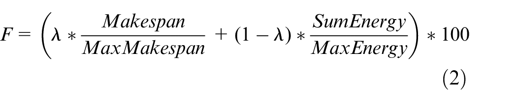
For chromosome mating, the GA uses the job-based order crossover (JOX) described in Bierwirth.¹⁸ Given two parents, JOX selects a random subset of jobs and copies their genes to the offspring in the same positions as they are in the first parent. Then the remaining genes are taken from the second parent so as they maintain their relative ordering. To clarify how JOX works, let us consider the following two parents in Figure 1 for the example presented in section ‘Example’.

Figure 1.

Result of crossover operator between two parents.

If the selected subset of jobs from the first parent just includes the job 2 (dark genes of parent 1 in Figure 1), the generated offspring is showed at the end of Figure 1.

Hence, operator JOX maintains for each machine a subsequence of operations in the same order as they are in parent 1 and the remaining in the same order as they are in parent 2.

The remaining elements of GA are rather conventional. To create a new generation, all chromosomes from the current one are organized into couples which are two mated offspring in accordance with the crossover probability.

Mutation operator

Two offspring generated with crossover operation can also be mutated in accordance the mutation probability. Two positions of the chromosome child are randomly chosen (position ‘a’ and position ‘b’), where ‘a’ must be lower than ‘b’. Values between ‘a’ and ‘b’ are randomly shuffled. Furthermore, in each gene, machine speed values are randomly changed. Finally, tournament replacement among every couple of parents and their offspring is carried out to obtain the next generation.

LS

Conventional GAs can produce good results. However, significant improvements can be obtained by hybridization with other methods. For example hybridization of a GA and an LS algorithm can produce better results because LS algorithms move from solution to solution in the search space by applying local changes. This is possible only if a neighbourhood relation is defined on the search space. An LS is implemented by defining a neighbourhood of each point in the search space as the set of chromosomes reachable by a given transformation rule. Then, a chromosome is replaced by the selected neighbour that satisfies the acceptance criterion. We propose a neighbourhood structure based on the concepts of critical path and critical block.^19–21 A critical block is a maximal subsequence of operations of a critical path requiring the same machine. Mattfeld²² defined the neighbourhood structure $N_{1}$ for JSP. It considers a set of moves called ‘interchange near the borderline of blocks on a single critical path’, what means swapping pairs of operations only at the beginning or at the end of a critical block.

Following the idea of neighbourhood structure $N_{1}$ and the concepts of critical path and critical block, we have defined the energy-efficient neighbourhood structure $(N_{EE})$ , where each task in the critical path is analysed to check if the next tasks of the same machine are consecutive and involved in the critical path. If this condition is met, a new neighbour is created swapping both tasks and the machine speed is increased if its fitness is not worsened. Furthermore, when a task is not in a critical path, its speed is decreased to create a new neighbour. An LS is only carried out if the runtime is bigger than the 80% of the given time-out.

A model for obtaining robust and energy-aware solutions

In this section, we propose a knowledge-based model to obtain robust and energy-aware solutions for the JSP with machines working at different speeds (JSMS).

Most scheduling problems involved in industrial processes are dynamic by nature. These dynamic problems are faced with incidences which generate delays in tasks. In some cases the original solution is recovered in a given time but in other cases the incidence is propagated in cascade so the original solution cannot be valid or recovered. Buffering is used in industrial processes to compensate for variations in the schedule. Changes in supply and demand would be an example of these variations. Think of buffering as a means to ensure that schedule continues to run smoothly despite unforeseen factors, such as machine breakdowns, coming into play. Thus, buffers in industrial processes are usually inserted to keep operations running smoothly. However, the inclusion of buffer in scheduling processes has advantages and disadvantages. The most important advantage of using buffering in scheduling is, when done correctly, its implementation tends to be more robust so, in order to increase production efficiency, reduce overall costs and keep operations running smoothly. However, when done incorrectly, the opposite can be true. For example, if a schedule keeps too much buffer time between all tasks, the makespan increases to remain the obtained solution not feasible in terms of profitability. To maintain an optimal balance, many operators tend to gravitate towards using industrial process strategies in which they use the least amount of buffering necessary to ensure their projected rates.

In this section, we transform the original scheduling model into a dual scheduling model in which some selected tasks are accomplished in a buffer time according to previous problem knowledge. The size of each buffer time assigned to a task is in accordance to the average duration of the previous disruptions generated in this task.

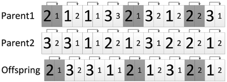
Figure 2 shows the different rates a machine can work for an assigned task Ti: green colour (speed 1) means that the machine works at lowest rate (lowest energy consumption), so the processing time is highest; yellow colour (speed 2) means that the machine works at regular rate, so the processing time is regular; and red colour (speed 3) means that the machine works at highest rate (highest energy consumption), so the processing time is lowest. Thus, the processing time of a task is dependent of the rate the assigned machine works. However, once the scheduling problem is solved and during execution, if an incidence occurs in task Ti, the assigned machine could increase its rate (if it was planned to work at speed 1 or 2) in order to absorb this incidence. Thus, the time interval between a given processing time and the lowest processing time of task Ti can be considered as an energy-efficient buffer.

Figure 2.

Processing time of a task in a machine working at different rates.

The dual scheduling model is aimed to insert additional buffer times to more dynamic tasks. To this end, the historical data are analysed to determine which tasks must be protected by a buffer time. Due the above advantages and disadvantages of the inclusion of buffer times, only the most dynamic tasks will be selected. Figure 3 shows the dual transformation of a dynamic task Ti. The dual transformation is composed of the following steps:

1. The original task model is composed of the number of tasks within the job (Ti), the assigned machine (Mx) and the different ways this machine can work (see Figure 2).

2. Modelling– if the task Ti is selected among the most dynamic ones, a dual task model $(Ti')$ is generated for this original task Ti. Thus, three buffer times are generated to task $Ti'$ according to the three processing times in which machine (Mx) can execute this dual task. Figure 4 shows possible combinations of three buffer times according to the size of the historical buffer time of original task Ti. Algorithm 1 shows how to calculate the actual buffer time assigned to each dual task. As can be seen in Figure 4, the historical buffer time is completely assigned to the dual task if it is executed at highest speed (diff3). Depending of the processing time of the dual task for regular and lowest speed, the buffer time is calculated according to Algorithm 1. Three different cases are shown in Figure 4. In Figure 4(a), it can be observed that the processing time at highest speed plus the historical buffer time is higher than the processing time at regular and lowest speed. In this case, all processing times are complemented with a buffer time in such a way that the sum of processing times and the assigned buffer time is equal in the three different speeds of the machine. The solver will be committed to select the green one (lowest speed) in order to minimize energy consumption. In Figure 4(b), it can be observed that the processing time at highest speed plus the historical buffer time is higher than the processing time at regular but not at lowest speed. In this case only a buffer time is assigned to dual tasks with highest and regular speeds. In Figure 4(c), it can be observed that the processing time at highest speed plus the historical buffer time is lower than the processing time at regular and lowest speed. In this case only a buffer time is assigned to dual tasks with highest speed.

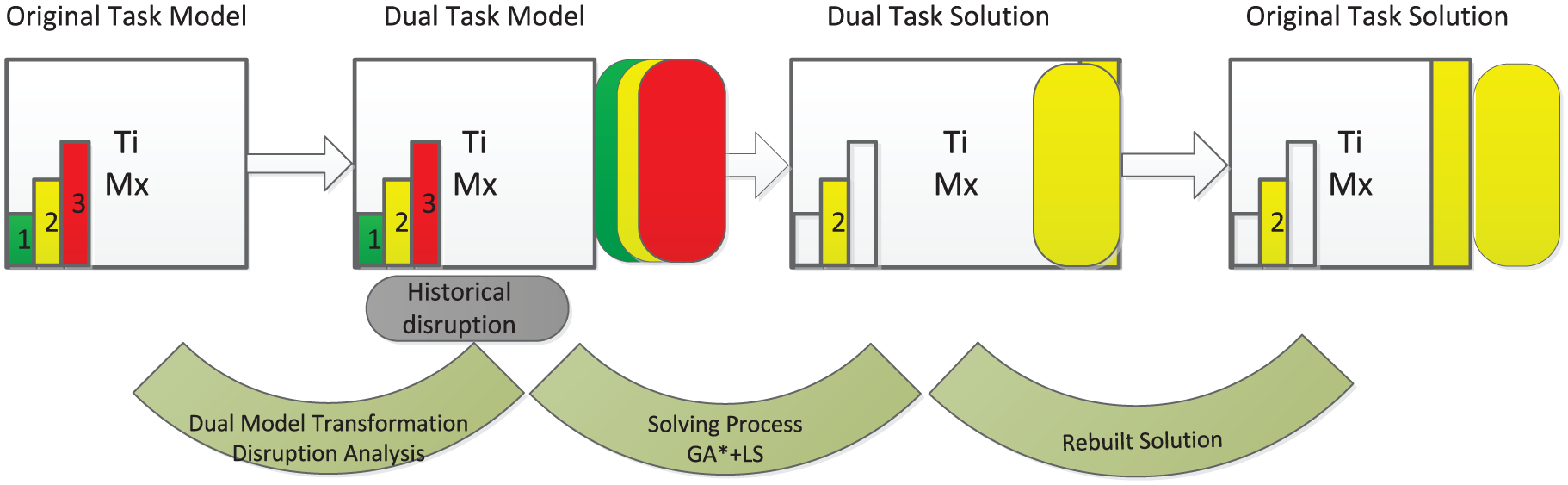
3. Solving– once the dual tasks $(Ti')$ are generated, they are grouped with the rest of the original tasks $(Ti)$ to generate the dual scheduling model. Our GA* + LS will be applied to obtain a Pareto front of the dual scheduling according to the parameter to be optimized: makespan and energy consumption. To this end, a convex combination between both parameters by a $λ \in [0, 1]$ value determined the Pareto front. Formula (2) shows the bi-criteria objective. Both parameters are normalized to balance the weight of both when $λ$ gets values around 0.5. In both cases, each parameter is divided by a maximum value.

Figure 3.

Dual transformation of a scheduling task.

Figure 4.

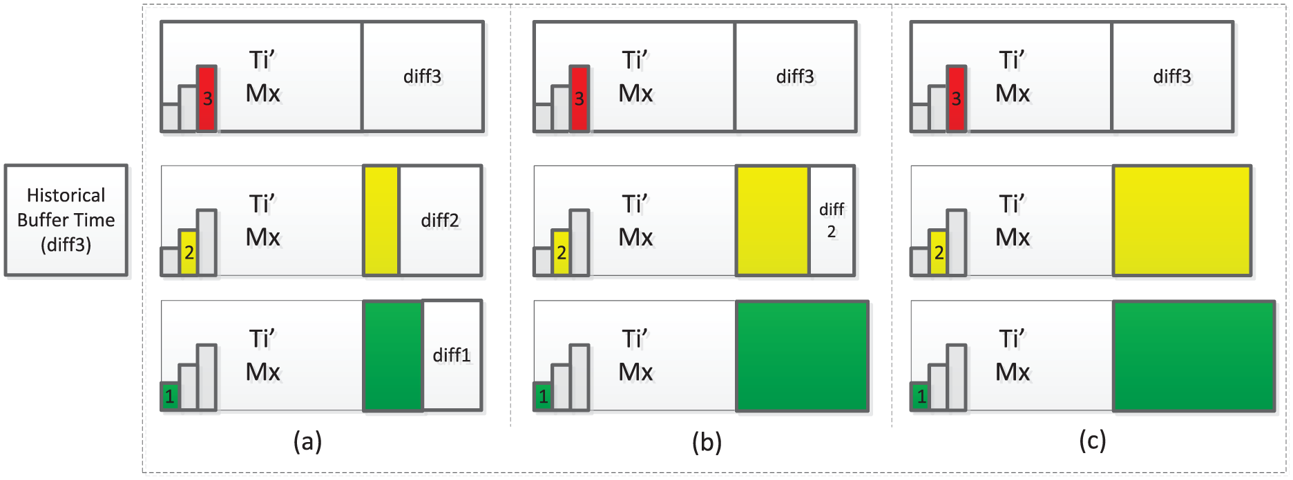
Three different cases for the buffer time assignment.

Algorithm 1: CalculateBufferTimes(Input (Tasks,BuffTime), Output (Tasks,BuffersTimes))
Begin
for (i=0;i < Ntasks;i++) do
if (isDynamic(Tasks[i])) then
if (BuffTime+Tasks[i].durSpeed3 > Tasks[i].durSpeed2) then
diff2=BuffTime+Tasks[i].durSpeed3-Tasks[i].durSpeed2;
end if
if (BuffTime+Tasks[i].durSpeed3 > Tasks[i].durSpeed1) then
diff1=BuffTime+Tasks[i].durSpeed3-Tasks[i].durSpeed1;
end if
diff3=BuffTime;
BuffersTimes[i]=[diff1,diff2,diff3];
end if
end for
End

It must be taken into account that any solver could be applied to the dual model. The selected solver is aimed to assign for each task, its start time, the processing time and the speed that the machine executes each task. Furthermore, the makespan and the energy consumption can be determined by the solver.

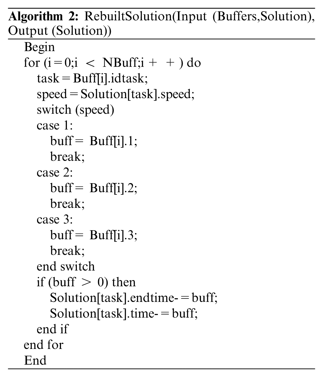
4. Rebuilt– once the obtained solutions are generated for the dual scheduling model, they are rebuilt to obtain solutions of the original scheduling model (see Figure 3). Thus, the robustness can be measured by decoupling the buffer times and the energy-efficient buffers generated in the schedule. This rebuilt task is formally presented in Algorithm 2.

Algorithm 2: RebuiltSolution(Input (Buffers,Solution), Output (Solution))
Begin
for (i=0;i < NBuff;i++) do
task=Buff[i].idtask;
speed=Solution[task].speed;
switch (speed)
case 1:
buff= Buff[i].1;
break;
case 2:
buff= Buff[i].2;
break;
case 3:
buff= Buff[i].3;
break;
end switch
if (buff > 0) then
Solution[task].endtime-=buff;
Solution[task].time-=buff;
end if
end for
End

Sometimes buffers can be generated close to a buffer time assigned in the dual model. So if the sum of both is higher than the maximum duration of the historical incidence, the speed of the assigned machine can be reduced (if possible) to get a more energy-aware solution with the same degree of robustness.

Example

In this section, a small example is shown to analyse and clarify the proposed model. Table 1 shows the processing time and the energy consumption for each rate/speed that each machine can work. The JSMS is composed of three jobs, three machines and three tasks per job. It must be taken into account that when the speed increases the energy consumption also increases, but the processing time decreases. For this example, 60 incidences were randomly generated. Table 2 shows the distribution of incidences among the most dynamic tasks (Column Nincidences). Only the more dynamic ones are selected to generate a dual model (the three tasks with more incidences, Job1-Task1, Job1-Task2 and Job3-Task1 are presented in Table 2).

Table 2.

Buffer times for most dynamic tasks.

Tasks	Nincidences	Buffer times
Tasks	Nincidences	Speed 1	Speed 2	Speed 3
Job1-Task1′	9	0	1	2
Job1-Task2′	10	0	0	2
Job3-Task1′	11	0	1	2

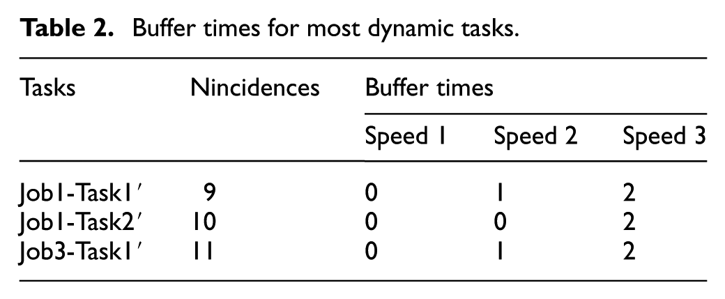
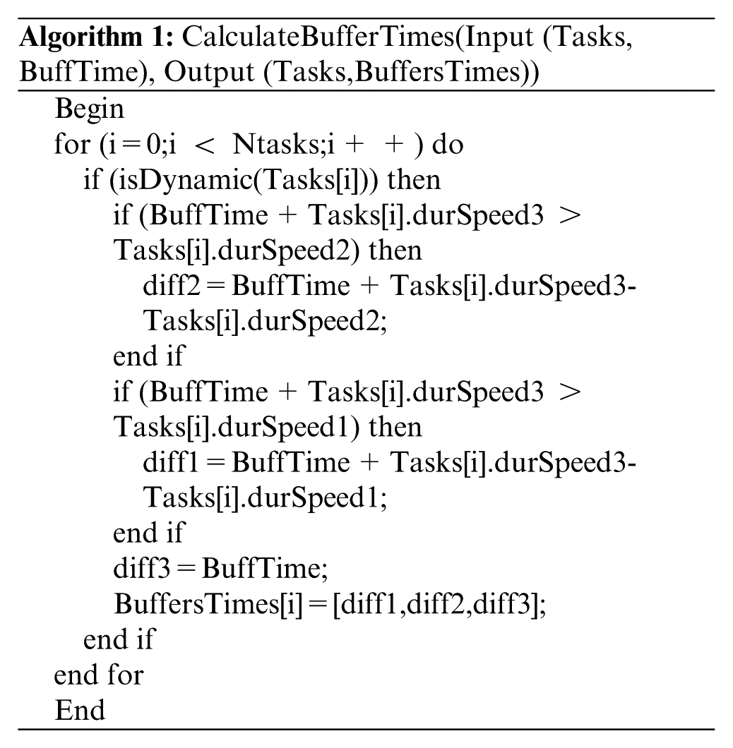
The historical buffer time will be calculated according to the historical disruptions. In this above set of 60 incidences, the average size of the disruption was 2. Thus, Algorithm 1 is executed to each selected dynamic task. The input of the algorithm is composed of the selected task and the average size of disruptions. Finally, the dual task model is obtained. This dual task model is composed of the original tasks with their corresponding processing time and the dual tasks with the original processing times plus the obtained buffer times shown in Table 2.

For example, Job1-Task1′ is a dual dynamic task with a buffer time assignment of type (b) according to Figure 4:

Buffer time at lowest speed is 0: the processing time of the original task at highest speed plus the historical buffer time is not bigger than the processing time at lowest speed.

Buffer time at regular speed is 1: The processing time of the original task at highest speed plus the historical buffer time is 1 unit bigger than the processing time at regular speed.

Buffer time at highest speed is 2: The processing time of the original task is increased with the historical buffer time (2 units).

Thus, the processing time of the dual tasks are updated by adding the calculated buffer times of Table 2. Then, the resultant dual model can be solved. Once the solution has been obtained, the dual tasks must rebuild to obtain the original processing times and their corresponding buffers.

Figure 5 shows the solution (Gantt chart) for the original example and the corresponding solution of the dual model. The assigned values of the processing time for the selected speed are shown in bold in Table 1. The buffer times are shown in grey blocks. The gaps are represented in black blocks. By comparing both solutions it can be observed that the energy consumption is the same and the makespan in the original model is 27 meanwhile in the dual model is 29. However, the solution obtained by the dual model is more robust due to the fact that almost all tasks (except Job2-Task3) are able to absorb incidences up to 2 time units.

Figure 5.

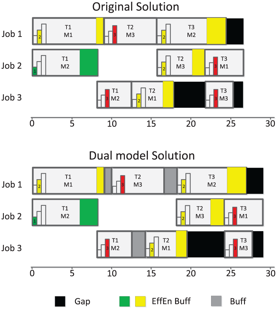
Original solution and dual model solution.

Evaluation

In this section, an evaluation of the proposed dual model is carried out to analyse and compare against the original model for finding robust and energy-aware solutions. As it has been pointed out, a memetic algorithm (GA* + LS) which combines a GA with an LS to solve the JSMS is applied. Furthermore, a comparative study was carried out by changing the value of buffer times to demonstrate that, as the buffer time increases, the robustness and energy efficiency also increase but the makespan decreases. Otherwise, stability is considered and solutions are analysed to know how incidences can be absorbed with the robustness and stable concepts.

Analysis of parameters

To carry out an extensive evaluation, two well-known benchmarks were used: Agnetis benchmarks²³ and Watson benchmarks.²⁴ In both cases, the instances were classified by the number of jobs $(j)$ , the number of machines $(m)$ , the number of tasks per job $(v_{\max})$ and the maximum processing times $(p)$ . In all Agnetis instances, the number of jobs was 3 and the instances were represented as m_ $v_{\max}$ _ p.

Agnetis instances are classified into two big groups, small and large:

Small: j = 3; m = 3, 5, 7; v_max = 5, 7, 10; p = (1, 10), (1, 50), (1, 100)

Large: j = 3; m = 3; v_max = 20, 25, 30; p = (1, 50), (1, 100), (1, 200)

In Watson instances, the number of jobs $(j)$ changes in all cases but m, $v_{\max}$ and p remain equal:

j = 50, 100, 200; m = 20; v_max = 20; p = (1, 100)

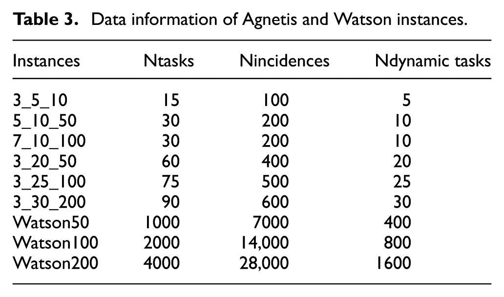
To simulate a historical background of the incidences for the Agnetis and Watson instances, a set of incidences were randomly assigned to tasks. To this end, the number of incidences was always proportional to the total number of tasks. Table 3 shows the analysed instances, the number of tasks, the number of simulated incidences and the number of selected dynamic tasks for the dual model. There must be a proportional relationship among the number of tasks, the number of simulated incidences and the number of selected dynamic tasks. The number of incidences must be significantly higher in order to classify and discriminate the more dynamic tasks. The number of dynamic tasks is also related to the number of tasks. A high number of dynamic tasks will generate a high degree of robustness but a worse makespan. As it was pointed out before, there must be equilibrium between the number of buffers and the optimality in terms of makespan.

Table 3.

Data information of Agnetis and Watson instances.

Instances	Ntasks	Nincidences	Ndynamic tasks
3_5_10	15	100	5
5_10_50	30	200	10
7_10_100	30	200	10
3_20_50	60	400	20
3_25_100	75	500	25
3_30_200	90	600	30
Watson50	1000	7000	400
Watson100	2000	14,000	800
Watson200	4000	28,000	1600

For each type of problem, 10 instances were evaluated, so the average results are shown in next tables. Original instances were extended as explained in Escamilla et al.⁷ New instances and more information can be found in the research group webpage (http://gps.webs.upv.es/jobshop/).

Comparative study

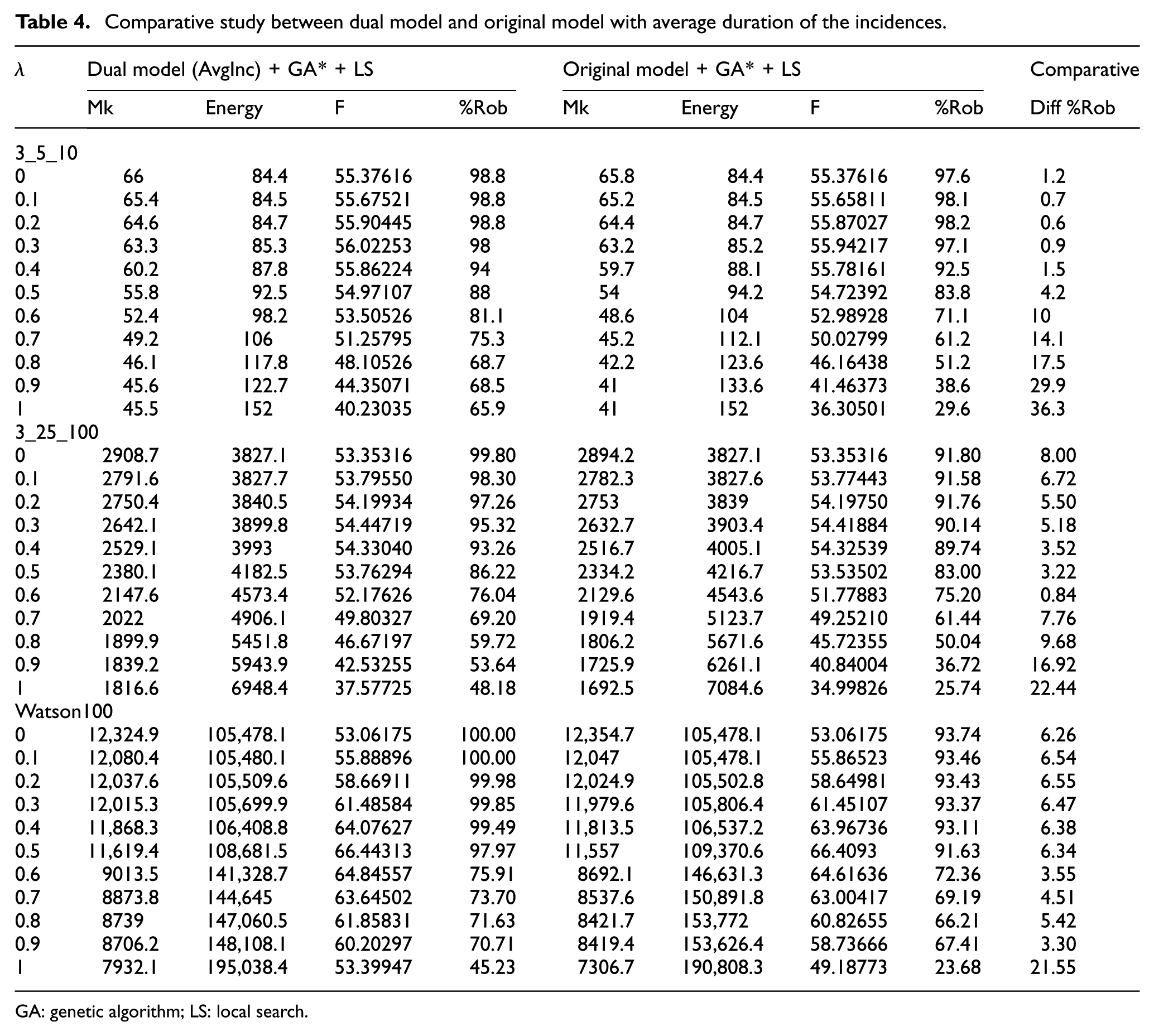
In this section, the behaviour of the dual model is compared against the original model. To this end, both models were executed over the same solver (GA* + LS) to analyse the performance of both models in terms of makespan, energy consumption and robustness. The incidences were randomly generated and assigned to tasks following the relation of Table 3. Once an incidence is assigned to a task, the duration is randomly generated between 1% and 20% of the maximum processing time for that instance. Thus, for instances where processing time was 50, the incidences were assigned a duration between 1 and 10. Table 4 shows the results for the Agnetis instances 3_5_10 and 3_25_100 and Watson100 instances. In all cases, the experiments were made over 10 different instances, so the values of the tables show average results. The values of robustness were also an average over the all incidences, so they are shown in percentage.

Table 4.

Comparative study between dual model and original model with average duration of the incidences.

$λ$	Dual model (AvgInc) + GA* + LS				Original model + GA* + LS				Comparative
$λ$	Mk	Energy	F	%Rob	Mk	Energy	F	%Rob	Diff %Rob
3_5_10
0	66	84.4	55.37616	98.8	65.8	84.4	55.37616	97.6	1.2
0.1	65.4	84.5	55.67521	98.8	65.2	84.5	55.65811	98.1	0.7
0.2	64.6	84.7	55.90445	98.8	64.4	84.7	55.87027	98.2	0.6
0.3	63.3	85.3	56.02253	98	63.2	85.2	55.94217	97.1	0.9
0.4	60.2	87.8	55.86224	94	59.7	88.1	55.78161	92.5	1.5
0.5	55.8	92.5	54.97107	88	54	94.2	54.72392	83.8	4.2
0.6	52.4	98.2	53.50526	81.1	48.6	104	52.98928	71.1	10
0.7	49.2	106	51.25795	75.3	45.2	112.1	50.02799	61.2	14.1
0.8	46.1	117.8	48.10526	68.7	42.2	123.6	46.16438	51.2	17.5
0.9	45.6	122.7	44.35071	68.5	41	133.6	41.46373	38.6	29.9
1	45.5	152	40.23035	65.9	41	152	36.30501	29.6	36.3
3_25_100
0	2908.7	3827.1	53.35316	99.80	2894.2	3827.1	53.35316	91.80	8.00
0.1	2791.6	3827.7	53.79550	98.30	2782.3	3827.6	53.77443	91.58	6.72
0.2	2750.4	3840.5	54.19934	97.26	2753	3839	54.19750	91.76	5.50
0.3	2642.1	3899.8	54.44719	95.32	2632.7	3903.4	54.41884	90.14	5.18
0.4	2529.1	3993	54.33040	93.26	2516.7	4005.1	54.32539	89.74	3.52
0.5	2380.1	4182.5	53.76294	86.22	2334.2	4216.7	53.53502	83.00	3.22
0.6	2147.6	4573.4	52.17626	76.04	2129.6	4543.6	51.77883	75.20	0.84
0.7	2022	4906.1	49.80327	69.20	1919.4	5123.7	49.25210	61.44	7.76
0.8	1899.9	5451.8	46.67197	59.72	1806.2	5671.6	45.72355	50.04	9.68
0.9	1839.2	5943.9	42.53255	53.64	1725.9	6261.1	40.84004	36.72	16.92
1	1816.6	6948.4	37.57725	48.18	1692.5	7084.6	34.99826	25.74	22.44
Watson100
0	12,324.9	105,478.1	53.06175	100.00	12,354.7	105,478.1	53.06175	93.74	6.26
0.1	12,080.4	105,480.1	55.88896	100.00	12,047	105,478.1	55.86523	93.46	6.54
0.2	12,037.6	105,509.6	58.66911	99.98	12,024.9	105,502.8	58.64981	93.43	6.55
0.3	12,015.3	105,699.9	61.48584	99.85	11,979.6	105,806.4	61.45107	93.37	6.47
0.4	11,868.3	106,408.8	64.07627	99.49	11,813.5	106,537.2	63.96736	93.11	6.38
0.5	11,619.4	108,681.5	66.44313	97.97	11,557	109,370.6	66.4093	91.63	6.34
0.6	9013.5	141,328.7	64.84557	75.91	8692.1	146,631.3	64.61636	72.36	3.55
0.7	8873.8	144,645	63.64502	73.70	8537.6	150,891.8	63.00417	69.19	4.51
0.8	8739	147,060.5	61.85831	71.63	8421.7	153,772	60.82655	66.21	5.42
0.9	8706.2	148,108.1	60.20297	70.71	8419.4	153,626.4	58.73666	67.41	3.30
1	7932.1	195,038.4	53.39947	45.23	7306.7	190,808.3	49.18773	23.68	21.55

GA: genetic algorithm; LS: local search.

Table 4 shows the makespan, energy consumption, F value and robustness of both models for different $λ$ values (see equation (2)). Thus, the Pareto front can be obtained for the multi-objective problem (makespan vs energy consumption). It must be taken into account that $λ = 0$ means that only energy consumption is taken into account so makespan is not considered, meanwhile $λ = 1$ means that only makespan is considered. In all analysed cases, it can be observed that makespan was always lower for the original model than the dual model. This is due to the fact that buffer times were inserted in the dual model to increase robustness, so the makespan was increased. For instance, the results for 3_5_10 in Table 4, for $λ = 1$ (only makespan is taken into account) show that the average makespan for the original model was 41 meanwhile the average makespan for the dual model was 45.5. In contrast, the value of robustness for the original model was 29.6% and the robustness for the dual model was 65.9%. So, with this instance, it is shown that by losing 4.5 units of makespan, the robustness was increased 36.3%. Something similar happens when only energy consumption was taken into account. However, the energy consumption was lower for the dual model than for the original model in most instances, mainly for $λ > 0.5$ . This is because the generated buffers during the solving process plus the previously assigned buffer times allowed machines to decrease their speed in the rebuilt phase.

In general, the solutions obtained by applying the dual model had a worse F value, but on other hand the solutions were more robust. Furthermore, it can be observed in the last column (Diff %Rob) that as the $λ$ value increases, the difference in robustness increased in a significant way. So, with the application of our dual model, it can be concluded that,

When only makespan was optimized, makespan was worsened but the robustness was improved.

When only the energy consumption was optimized, the robustness was improved without losing optimality.

When both variables were optimized, makespan was worse but energy consumption had a different behaviour, but robustness was improved.

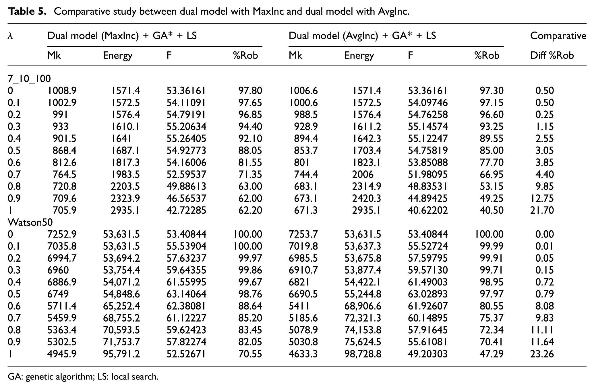
Table 5 shows the results of Agnetis instances 7_10_100 and Watson50 instances to analyse the behaviour of the dual model over the size of the buffer times. To this end, two different buffer time sizes were analysed: buffer times with the maximum duration size of the incidences (MaxInc) and buffer times with the average size of all incidences (AvgInc). This table represents the behaviour of all instances analysed in Table 3 and all instances showed a similar behaviour.

Table 5.

Comparative study between dual model with MaxInc and dual model with AvgInc.

$λ$	Dual model (MaxInc) + GA* + LS				Dual model (AvgInc) + GA* + LS				Comparative
$λ$	Mk	Energy	F	%Rob	Mk	Energy	F	%Rob	Diff %Rob
7_10_100
0	1008.9	1571.4	53.36161	97.80	1006.6	1571.4	53.36161	97.30	0.50
0.1	1002.9	1572.5	54.11091	97.65	1000.6	1572.5	54.09746	97.15	0.50
0.2	991	1576.4	54.79191	96.85	988.5	1576.4	54.76258	96.60	0.25
0.3	933	1610.1	55.20634	94.40	928.9	1611.2	55.14574	93.25	1.15
0.4	901.5	1641	55.26405	92.10	894.4	1642.3	55.12247	89.55	2.55
0.5	868.4	1687.1	54.92773	88.05	853.7	1703.4	54.75819	85.00	3.05
0.6	812.6	1817.3	54.16006	81.55	801	1823.1	53.85088	77.70	3.85
0.7	764.5	1983.5	52.59537	71.35	744.4	2006	51.98095	66.95	4.40
0.8	720.8	2203.5	49.88613	63.00	683.1	2314.9	48.83531	53.15	9.85
0.9	709.6	2323.9	46.56537	62.00	673.1	2420.3	44.89425	49.25	12.75
1	705.9	2935.1	42.72285	62.20	671.3	2935.1	40.62202	40.50	21.70
Watson50
0	7252.9	53,631.5	53.40844	100.00	7253.7	53,631.5	53.40844	100.00	0.00
0.1	7035.8	53,631.5	55.53904	100.00	7019.8	53,637.3	55.52724	99.99	0.01
0.2	6994.7	53,694.2	57.63237	99.97	6985.5	53,675.8	57.59795	99.91	0.05
0.3	6960	53,754.4	59.64355	99.86	6910.7	53,877.4	59.57130	99.71	0.15
0.4	6886.9	54,071.2	61.55995	99.67	6821	54,422.1	61.49003	98.95	0.72
0.5	6749	54,848.6	63.14064	98.76	6690.5	55,244.8	63.02893	97.97	0.79
0.6	5711.4	65,252.4	62.38081	88.64	5411	68,906.6	61.92607	80.55	8.08
0.7	5459.9	68,755.2	61.12227	85.20	5185.6	72,321.3	60.14895	75.37	9.83
0.8	5363.4	70,593.5	59.62423	83.45	5078.9	74,153.8	57.91645	72.34	11.11
0.9	5302.5	71,753.7	57.82274	82.05	5030.8	75,624.5	55.61081	70.41	11.64
1	4945.9	95,791.2	52.52671	70.55	4633.3	98,728.8	49.20303	47.29	23.26

GA: genetic algorithm; LS: local search.

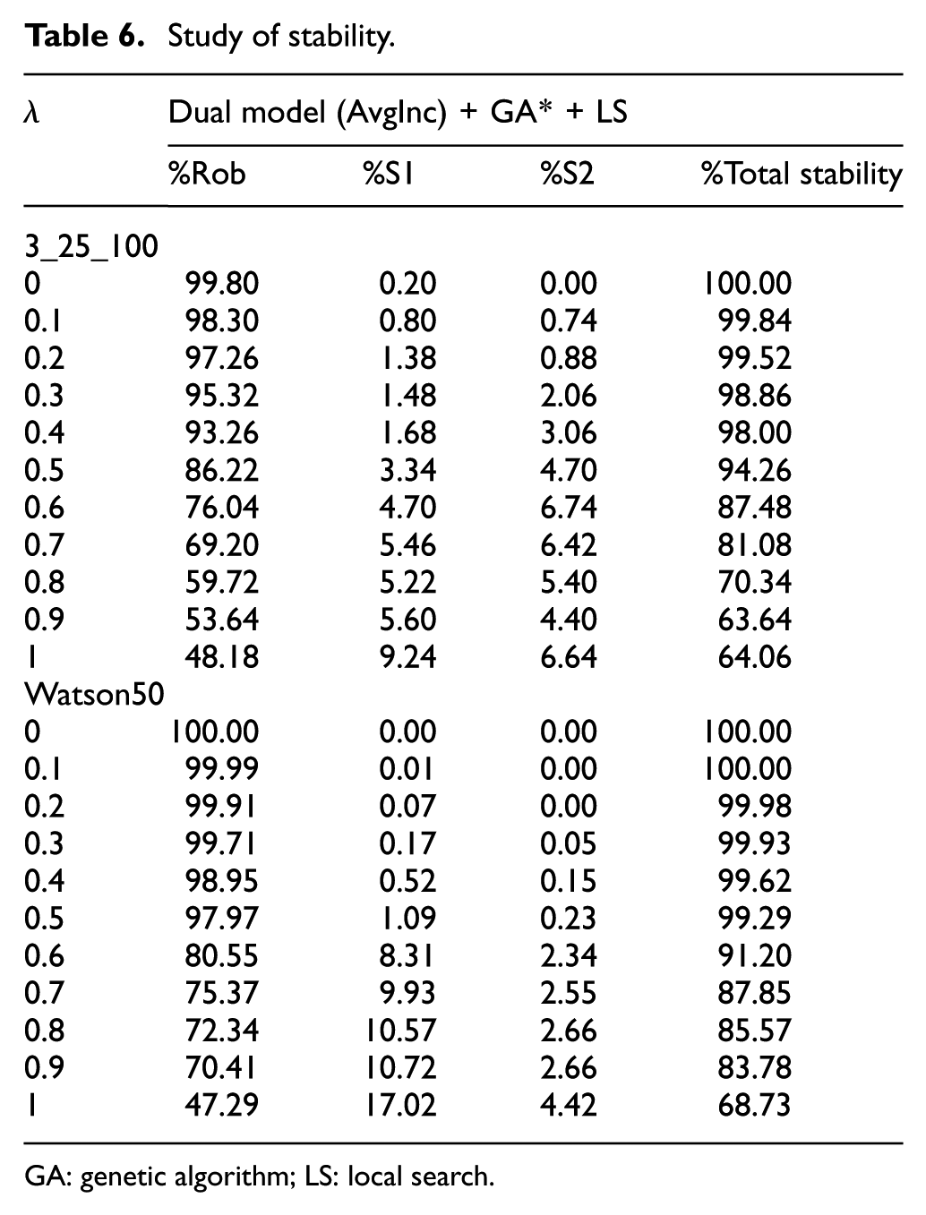
The dual model with MaxInc had an F value higher than the dual model with AvgInc. However, the robustness value was always higher in the dual model with MaxInc. This is because, as the buffer time of the MaxInc was always bigger than AvgInc, the makespan value was also higher and thus the F value. For example for $λ = 1$ in Table 5 (7_10_100), it can be seen that the difference between both makespan was 34.6 but the difference between robustness was 21.70%.

Finally, the stability was analysed for the dual model in both Agnetis and Watson instances. As it was pointed out in section ‘Robustness and stability’, stability is the ability of a solution to recover with only a few changes. Thus, given an incidence in a task Ti, 0-stable is equivalent to robustness, so no further tasks will be affected, meanwhile 1-stable and 2-stable require to change the start time of 1 $(Tj)$ and 2 tasks $(Tk, Tp)$ , respectively.

Table 6 shows the percentage of robustness or 0-stability (%Rob), 1-stability (%S1) and 2-stability (%S2), and the percentage of total stability (%Total Stability) obtained by summing up the three previous parameters for Agnetis instances 3_25_100 and Watson50 instances. The rest of instances presented in Table 3 maintained similar behaviours. It can be observed that robustness or 0-stability (%Rob) had a higher value than 1-stability (%S1) and 2-stability (%S2). This is due to the fact that, the dual model was designed to add buffer times to more dynamic tasks. Thus, given an incidence, the algorithm tried to absorb it by increasing the speed of the machine or by using the assigned buffer time. If the incidence was not able to be absorbed, it was checked whether the incidence could be absorbed by the next task of the same machine or by the next task of the same job. If the incidence can be absorbed by changing only one task (from the same machine or the same job), it is considered a 1-stable solution. However, if both tasks have to be modified, it is considered a 2-stable solution. For both Agnetis and Watson instances, the percentage of total stability was close to 100% for $λ$ values lower than 0.5. For example, when $λ = 0$ , all incidences were absorbed with 0, 1 or 2 changes in the original solutions, achieving a 100% of total stability in both instances. Furthermore, as $λ$ values increased (the makespan was minimized), the percentage of robustness decreased and more incidences were not able to be absorbed. However, the 1-stability and 2-stability increased to absorb some of the incidences that were not directly absorbed by the dual model. For instance, in Watson50 instances, for $λ = 1$ , percentage of total stability increased a 21.44% with respect to robustness (47.29%), achieving a total percentage of stability of 68.73%.

Table 6.

Study of stability.

$λ$	Dual model (AvgInc) + GA* + LS
$λ$	%Rob	%S1	%S2	%Total stability
3_25_100
0	99.80	0.20	0.00	100.00
0.1	98.30	0.80	0.74	99.84
0.2	97.26	1.38	0.88	99.52
0.3	95.32	1.48	2.06	98.86
0.4	93.26	1.68	3.06	98.00
0.5	86.22	3.34	4.70	94.26
0.6	76.04	4.70	6.74	87.48
0.7	69.20	5.46	6.42	81.08
0.8	59.72	5.22	5.40	70.34
0.9	53.64	5.60	4.40	63.64
1	48.18	9.24	6.64	64.06
Watson50
0	100.00	0.00	0.00	100.00
0.1	99.99	0.01	0.00	100.00
0.2	99.91	0.07	0.00	99.98
0.3	99.71	0.17	0.05	99.93
0.4	98.95	0.52	0.15	99.62
0.5	97.97	1.09	0.23	99.29
0.6	80.55	8.31	2.34	91.20
0.7	75.37	9.93	2.55	87.85
0.8	72.34	10.57	2.66	85.57
0.9	70.41	10.72	2.66	83.78
1	47.29	17.02	4.42	68.73

GA: genetic algorithm; LS: local search.

Conclusion

Industrial processes involve a large number of task scheduling problems. JSPs where machines can work at different rates/speeds (JSMS) represent a large number of combinatorial problems in industrial processes. In this article, a dual model is proposed to relate optimality criteria with energy consumption and robustness/stability. This model is committed to protect dynamic tasks against further incidences in order to obtain robust and energy-aware solutions. The proposed dual model has been evaluated with a memetic algorithm (GA* + LS) to compare the behaviour against the original model. The result shows that the proposed dual model was able to obtain more robust solutions in all instances and more energy-efficient solutions in most of them. This is due to the fact that the assigned buffer times to some tasks are used to protect them against incidences. Furthermore, if during execution, there is no incidence, the involved machine can use this buffer to work at lower speed, so the energy consumption can be also reduced. The combination of robustness and stability gives the proposal an added value because although an incidence cannot be directly absorbed by the disrupted task, it can be repaired by involving only a small number of tasks. Thus the original solution can be recovered in order to maintain feasible the rest of the obtained schedule.

Footnotes

Declaration of conflicting interests

The author(s) declared no potential conflicts of interest with respect to the research, authorship and/or publication of this article.

Funding

The author(s) disclosed receipt of the following financial support for the research, authorship, and/or publication of this article: This research has been supported by the Spanish Government under research project TIN2013-46511-C2-1 for the Spanish government and the TETRACOM EU project FP7-ICT-2013-10-No 609491.

References

Chen

Zhang

Arinez

et al . Energy-efficient production systems through schedule-based operations. IEEE T Autom Sci Eng 2013; 10(1): 27–37.

Newman

Nassehi

Imani-Asrai

et al . Energy efficient process planning for CNC machining. CIRP J Manuf Sci Technol 2012; 5(2): 127–136.

Administration, U. E. I. (2013). International Energy Outlook 2013. Report Number: DOE/EIA-0484.

Wang

Ding

Qiu

et al . A low-carbon production scheduling system considering renewable energy. In: Proceedings of the 2011 IEEE international conference on service operations, logistics, and informatics (SOLI), Beijing, China, 10–12 July 2011, pp.101–106. New York: IEEE.

et al . An energy-responsive optimization method for machine tool selection and operation sequence in flexible machining job shops. J Clean Prod 2015; 87: 245–254.

May

Stahl

Taisch

et al . Multi-objective genetic algorithm for energy-efficient job shop scheduling. Int J Prod Res 2015; 53: 7071–7089.

Escamilla

Salido

Giret

et al . A metaheuristic technique for energy-efficiency in job-shop scheduling. In: Proceedings of the workshop on constraint satisfaction techniques (COPLAS) 2014: 24th international conference on automated planning and scheduling (ICAPS), Portsmouth, NH, 21–26 June 2014, pp.42–50. AAAI.

Mingcheng

Jiang

Zuo

Study on multi-objective flexible job-shop scheduling problem considering energy consumption. J Ind Eng Manag 2014; 3(7): 589–604.

Liu

Dong

Lohse

et al . An investigation into minimising total energy consumption and total weighted tardiness in job shops. J Clean Prod 2014; 65: 87–96.

10.

Petrovic

Ouelhadj

A survey of dynamic scheduling in manufacturing systems. J Ind Eng Manag 2009; 4(12): 417–431.

11.

Pach

Berger

Sallez

et al . Reactive and energy-aware scheduling of flexible manufacturing systems using potential fields. Comput Ind 2014; 65(3): 434–448.

12.

Zheng

Tang

Giret

et al . Dynamic shop floor re-scheduling approach inspired by a neuroendocrine regulation mechanism. Proc IMechE, Part B: J Engineering Manufacture 2015; 229: 121–134.

13.

Blazewicz

Cellary

Slowinski

et al . Scheduling under resource constraints-deterministic models. Ann Oper Res 1986; 7: 1–356.

14.

Jen

Stable or robust? Whats the difference?

Complexity 2003; 8(3): 12–18.

15.

Barber

Salido

MA.

Robustness, stability, recoverability, and reliability in constraint satisfaction problems. Knowl Inf Syst 2015; 44(3): 719–734.

16.

Beasley

Martin

Bull

DR.

An overview of genetic algorithms: part 1, fundamentals. U Comput 1993; 15: 58–69.

17.

Varela

Serrano

Sierra

New codification schemas for scheduling with genetic algorithms. In: Mira

Álvarez

(eds) Artificial intelligence and knowledge engineering applications: a bioinspired approach. Berlin, Heidelberg: Springer-Verlag, 2005, pp.11–20.

18.

Bierwirth

A generalized permutation approach to job shop scheduling with genetic algorithms. OR Spectrum 1995; 17: 87–92.

19.

Matsuo

Suh

Sullivan

RS.

A controlled search simulated annealing method for the general job-shop scheduling problem. Austin, TX: Graduate School of Business, University of Texas, 1988.

20.

Van Laarhoven

PJM

Aarts

EHL

Lenstra

JK.

Job shop scheduling by simulated annealing. Oper Res 1992; 40(1): 113–125.

21.

Nowicki

Smutnicki

A fast taboo search algorithm for the job shop scheduling problem. Manage Sci 1996; 42: 797–813.

22.

Mattfeld

DC.

Evolutionary search and the job shop: investigations on genetic algorithms for production scheduling. Berlin, Heidelberg: Springer-Verlag, 1995.

23.

Agnetis

Flamini

Nicosia

et al . A job-shop problem with one additional resource type. J Sched 2011; 14(3): 225–237.

24.

Watson

J-P

Barbulescu

Howe

et al . Algorithm performance and problem structure for flow-shop scheduling. In: Proceedings of the sixteenth national conference on artificial intelligence and the eleventh innovative applications of artificial intelligence conference innovative applications of artificial intelligence (AAAI’99/IAAI’99), Orlando, FL, 18–22 June 1999, pp.688–695. Palo Alto, CA: AAAI.

A dual scheduling model for optimizing robustness and energy consumption in manufacturing systems

Abstract

Keywords

Introduction

Problem description

Robustness and stability

Memetic algorithm (GA* + LS)

Chromosome encoding and decoding

Initial population and fitness

Crossover operator

Mutation operator

LS

A model for obtaining robust and energy-aware solutions

Example

Evaluation

Analysis of parameters

Comparative study

Conclusion

Footnotes

Declaration of conflicting interests

Funding

References