Sage Journals: Discover world-class research

Abstract

Several control charts have been constructed to simultaneously monitor the process mean and variability. A single chart is often used instead of two charts to detect shift in the process mean and variability separately. A new single generally weighted moving average control chart is now proposed to monitor the process mean and dispersion simultaneously, based on Taguchi’s loss function. A Monte Carlo simulation is used to calculate average run length to study the performance of this control chart when the process is shifted. A comparison is made with an exponentially weighted moving average control chart in terms of average run lengths. Two examples are also included for showing the practical application of the proposed control chart.

Keywords

Control chart average run length loss function Monte Carlo simulation

Introduction

Control charts play an important role in statistical process control (SPC), particularly when to monitor the sensitivity of the process to enhance the quality of products manufactured specially in industries using today’s modern technologies. Many control charts such as by Aslam et al.,^1,2 Azam et al.,³ Haq et al.,⁴ Huang et al.,⁵ Huwang et al.,⁶ Ou et al.⁷ and Sheu and Hsieh⁸ have now been developed to monitor the process mean and/or variability and to detect a shift in the process. Exponentially weighted moving average (EWMA) control charts or cumulative sum (CUSUM) control charts are often used for detecting small shifts in the process.⁹ The work started by Shewhart in 1924 has now many different dimensions such as double/multiple sampling control chart schemes, repetitive control chart schemes and use of process capability and loss functions in control charts, some of which can be seen in Ahmad et al.,¹⁰ Al-Refaie et al.,¹¹ Aslam et al.,¹² Castagliola and Vannman,¹³ Khoo et al.,¹⁴ Ouyang et al.,¹⁵ and Yeong et al.,¹⁶ which are now quiet helpful methodologies to detect small shifts in the process.

Many studies have been conducted to simultaneously monitor the process mean and variability using a single control chart, which helps to reduce the required time, cost, labor and resources. To list a few, recent works include the Max-EWMA chart by Chen et al.,¹⁷ the EWMA semi-circle (EWMA-SC) chart by Chen et al.,¹⁸ a loss function–based control chart by Wu and Tian,^19,20 a CUSUM control chart based on Taguchi’s loss function by Jiao and Helo,²¹ a combination of generally weighted moving average (GWMA) chart by Sheu et al.,²² the sum of squares double EWMA chart by Teh et al.,²³ the extended maximum GWMA charts by Sheu et al.,²⁴ a GWMA chart by Teh et al.,²⁵ the X control chart by Yang et al.,²⁶ the variable sampling interval (VSI) average loss control chart by Yang²⁷ and the extended VSI EWMA average loss control chart diagnosing the source of out-of-control process by Yang.²⁸

Roberts²⁹ first analyzed that EWMA is helpful to detect small shift in the process mean. Sheu and Griffith³⁰ and Sheu^31,32 applied a new method to EWMA control chart to detect an out-of-control signal in the process as quickly as possible, and later Sheu and Lin³³ called this expanded EWMA control chart as GWMA control chart, which is more sensitive than EWMA control chart in detecting small shifts. Their GWMA control chart can also locate small shifts in the initial process because of an additional adjustment parameter α.

Loss function plays a vital role to measure the manufacturing cost of the products which can deviate due to variability in the quality characteristics of the products because it is a definite part of the manufacturing process.³⁴ Usually, when all products fall within the specification limits of a process, it is considered that they possess the same quality characteristics. However, a quality characteristic of a product closer to its target value will lead a smaller quality cost than those ones which are closer to the lower or upper specification limit.³⁵

By exploring the literature, it comes to our knowledge that there is no work for the control charts based on GWMA statistic using the Taguchi loss function. Yang²⁸ proposed the VSI EWMA average loss control chart and diagnosed the source of out-of-control process. In this article, it is assumed that the process mean even when it is in control is not equal to the target value of the process, which is often true in practice. The purpose of this article is to develop a new GWMA control chart using Taguchi’s philosophy³⁶ of the quality characteristic to identify an out-of-control signal when it deviates from its target value. Moreover, it would also be helpful to diagnose an out-of-control signal either in the process mean or the variability or both simultaneously using a single chart.

The rest of the article is organized as follows: section “Design of GWMA control chart using Taguchi loss function” describes the proposed control chart based on GWMA and the Taguchi loss function. In section “Performance and evaluation,” the results of the proposed control chart are discussed and are compared with VSI EWMA control chart in Yang²⁸ in terms of its average run lengths (ARLs) using a simulation study. Two illustrative examples are included in section “Examples” for practical application of the proposed control chart and section “Conclusion” elaborates the conclusion.

Design of GWMA control chart using Taguchi loss function

Taguchi loss function

Following Yang,^27,28 let us suppose that the quality characteristic X follows a normal distribution with mean µ and variance σ² when the process is in control, that is, X ∼ N (µ, σ²). Then, the Taguchi’s quadratic loss function is given as

L_{e} = k' (X - T^{*})^{2}

(1)

where $k'$ is the proportionality constant, and T^* is the target value. According to Taguchi, this function represents the loss incurred by the consumer, the producer and the society.³⁷

Now, it is important to express this loss function in terms of process location and process dispersion. So, Chandra³⁷ derived the expected value of this loss function (1) which can be written as

EL = E (L_{e}) = k' [σ^{2} + {(μ - T^{*})}^{2}]

(2)

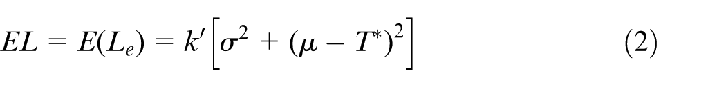
where $k'$ is the proportionality constant, T^* is the target value (as mentioned above) and $μ$ and $σ^{2}$ represent the true values of process location and variability, respectively.

Most of the time, it is necessary to use the estimates of µ and σ² when their true values are unknown; then according to Yang,^27,28 this expected loss (EL) is estimated as

{\hat{L}}_{e} = k' [\frac{(n - 1)}{n} S^{2} + {(\bar{X} - T^{*})}^{2}]

(3)

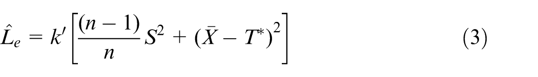
which is an unbiased estimator of EL,^27,28 where $S^{2} = (\sum_{i = 1}^{n} (X_{i} - \bar{X})^{2}) / (n - 1)$ and $\bar{X} = (\sum_{i = 1}^{n} X_{i}) / n$ are the sample variance and sample mean, respectively.

As discussed by Yang,^27,28 ${\hat{L}}_{e} ~ (k' σ^{2} χ_{n, θ_{0}}^{2}) / n$ because S² and $\bar{X}$ are independent, where $χ_{n, θ_{0}}^{2}$ is a non-central chi-square distribution with n degrees of freedom and non-centrality parameter $θ_{0} = n ((μ - T^{*}) / σ)^{2}$ . If we define $ν = (μ - T^{*}) / σ$ , then $θ_{0} = n ν^{2}$ . Yang^27,28 transformed the in-control statistics ${\hat{L}}_{e}$ to L by

L = \frac{n {\hat{L}}_{e}}{k' σ^{2}} ~ χ_{n, θ_{0}}^{2}

(4)

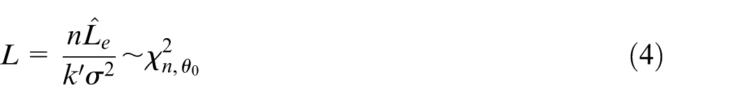
And assume that $k' = 1$ , thus

L = \frac{n {\hat{L}}_{e}}{σ^{2}} ~ χ_{n, θ_{0}}^{2}

(5)

Without loss of generality, it can be assumed that the process mean shifts to the right and the variance increases, that is, $X ~ N (μ + ξ σ, ρ^{2} σ^{2})$ , for $ξ \geq 0$ and $ρ \geq 1$ , when the process is out of control. Thus, Yang^27,28 transformed L under the shifted process as

L = \frac{n {\hat{L}}_{e}}{σ^{2}} ~ χ_{n, θ_{1}}^{2}

(6)

where $θ_{1} = n ((μ + ξ σ - T^{*}) / (ρ σ))^{2} = n ((ν + ξ) / ρ)^{2}$

GWMA of Taguchi loss

Let M count the number of samples until the first occurrence of an event of interest. According to Sheu and Lin,³³ $P (M = j)$ is treated as the weight assigned to each previous sample in the weighted moving average. So, $P (M = 1)$ is the weight assigned to the current sample, and $P (M = 2)$ is the weight assigned to the previous sample and so on. Let $L_{j}$ be the Taguchi’s estimated loss at time (sample) j. Then, the GWMA of the Taguchi loss at time j will be given by

\begin{array}{l} U_{j} = P (M = 1) L_{j} + P (M = 2) L_{j - 1} + … + \\ P (M = j) L_{1} + P (M > j) U_{0}, j = 1, 2, 3… \end{array}

where $U_{0}$ is the true process mean, that is, $U_{0} = (n + θ_{0})$ .

Let us define

{\bar{P}}_{j} = P (M > j), j = 0, 1, 2, \dots ({\bar{P}}_{0} = 1)

Then

P (M = j) = {\bar{P}}_{j - 1} - {\bar{P}}_{j} = {\bar{P}}_{j - 1} (1 - \frac{{\bar{P}}_{j}}{{\bar{P}}_{j - 1}})

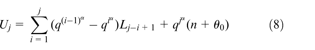
Now, the GWMA of the Taguchi loss at time j will be

\begin{array}{l} U_{j} = ({\bar{P}}_{0} - {\bar{P}}_{1}) L_{j} + ({\bar{P}}_{1} - {\bar{P}}_{2}) L_{j - 1} + … + \\ ({\bar{P}}_{j - 1} - {\bar{P}}_{j}) L_{1} + {\bar{P}}_{j} U_{0} \end{array}

(7)

If $({\bar{P}}_{0} - {\bar{P}}_{1}) > ({\bar{P}}_{1} - {\bar{P}}_{2}) > \dots > ({\bar{P}}_{j - 1} - {\bar{P}}_{j})$ , then this means that the maximum weight is assigned to the current sample, and smaller weights are assigned to the previous samples, and the least weight is assigned to the most remote sample.

As discussed by Sheu and Lin,³³ we will take the form of ${\bar{P}}_{j} = q^{j^{α}}$ , where design parameter q is a constant such that $0 < q \leq 1$ and α is an adjustment parameter determined by the practitioner. Thus, equation (7) becomes

U_{j} = \sum_{i = 1}^{j} (q^{{(i - 1)}^{α}} - q^{i^{α}}) L_{j - i + 1} + q^{j^{α}} (n + θ_{0})

(8)

When $α = 1$ , it reduces to a EWMA scheme.

Proposed control chart based on GWMA of Taguchi loss

Since $L = (n {\hat{L}}_{e}) / (σ^{2}) ~ χ_{n, θ_{0}}^{2}$ , the starting value $U_{0}$ will be set as the mean of L, that is, $U_{0} = (n + θ_{0})$ and lower control limit (LCL) is set to be 0 because L cannot be negative. The upper control limit (UCL) is set up as follows

UCL = E (U_{j}) + k \sqrt{V (U_{j})}

where k is a constant to be determined by specifying the values of design parameters α and q at fixed value of in-control ARL. The mean and the variance of U_j are

E (U_{j}) = (n + θ_{0})

(9)

and

V (U_{j}) = D_{j} {2 (n + 2 θ_{0})}

(10)

where $D_{j} = ({\bar{P}}_{0} - {\bar{P}}_{1})^{2} + ({\bar{P}}_{1} - {\bar{P}}_{2})^{2} + \dots + ({\bar{P}}_{j - 1} - {\bar{P}}_{j})^{2}$ . For the choice of ${\bar{P}}_{j} = q^{j^{α}} (0 < q < 1, α > 0)$ , $D_{j} = (q^{0^{α}} - q^{1^{α}})^{2} + (q^{1^{α}} - q^{2^{α}})^{2} + \dots + (q^{{(j - 1)}^{α}} - q^{j^{α}})^{2}$

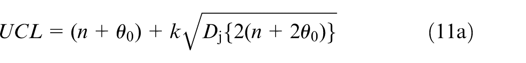
The value of $D_{j}$ converges as j increases although the limit cannot be evaluated in a closed form.

Hence, UCL and LCL can be written as

UCL = (n + θ_{0}) + k \sqrt{D_{j} {2 (n + 2 θ_{0})}}

(11a)

LCL = 0

(11b)

If any $U_{j} > UCL$ , then the process is declared to be out of control. The design parameters of the chart are k, α and q, which control the performance of the chart for fixed sample size n.

Now when $μ = T^{*}$ , this implies that $θ_{0} = 0$ ; the EWMA-SC chart proposed by Chen et al.¹⁸ becomes a special case fixed parameter (FP) EWMA average loss chart.²⁷ So this GWMA average loss control chart will also become a general case of the EWMA-SC chart when $μ = T^{*}$ , and thus the control limits are then given by

UCL = n + k \sqrt{D_{j} (2 n)}

(12a)

LCL = 0

(12b)

Hence, the charting procedure of GWMA average loss chart is given in the following different steps:

If µ and σ are unknown, then use their estimates $\bar{\bar{x}}$ and $\bar{S} / c_{4}$ , respectively. And ${\bar{S}}^{2}$ is used for σ² if it is unknown. Here, $\bar{\bar{x}} = ({\bar{x}}_{1} + {\bar{x}}_{2} + \dots + {\bar{x}}_{m}) / m$ is the overall mean of the sample means of m preliminary subgroups and $\bar{S} = (S_{1} + S_{2} + \dots + S_{m}) / m$ is the overall mean of the standard deviations of m preliminary subgroups.

In an initial stage, specify the target value T^* and an in-control ARL (ARL₀) to obtain an optimal value of k with the specified values of (q, α) for fixed sample size n to make a combination of (q, α, k) using simulation.

Calculate the UCL of the proposed control chart using equation (11a).

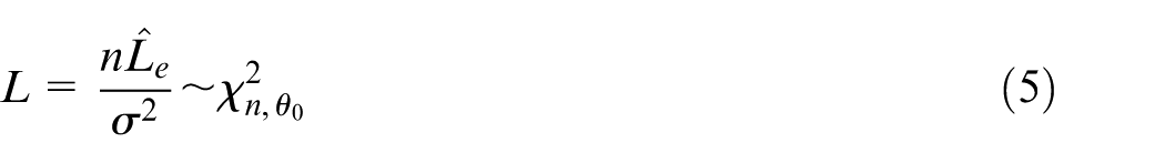
Compute L from equation (5) in order to calculate the plotting statistic U_j using equation (8) with the help of combination of (q, α, k) obtained in Step 2. Plot the statistic U_j against each subgroup j = 1, 2, 3,… (where the choice of j is dependent on the shift to be detected). If any U_j ≥ UCL, then highlight the point(s) which exceeds from UCL.

Analyze and identify the cause(s) of each out-of-control signal which may be due to an increase in process mean or process dispersion or both which can be decided by shifts to be diagnosed.

Performance and evaluation

Performance of a control chart is generally evaluated by the ARL,^29,38 which indicates how many points to be plotted before providing an out-of-control signal. Usually, ARL needs to be sufficiently large to avoid false alarms when the process is in control and should be small if it wants to detect an out-of-control signal quickly. In this study, µ = 0 and σ² = 1 are used for the in-control process and out-of-control signal; shift is involved in the process mean or in the standard deviation or in both simultaneously to find out-of control ARL (ARL₁).

Markov chain approach or integral equation approach is frequently applied to calculate ARLs in many literatures. However, a Monte Carlo simulation is conducted to estimate the ARLs because Markov chain approach or integral equation approach is difficult to evaluate for this chart. In all, 10,000 iterations are performed to evaluate each ARL and each iteration is stopped when a point indicates an out-of-control signal (exceeds from UCL) for the value of k until the required ARL₀ is obtained.

Without loss of generality, the subgroup size is taken as n = 5. The random variable X_ji (j = 1, 2, 3,… and i = 1, 2, 3,…, n) is distributed as independent normal variate with mean µ and variance σ². The shift $ξ σ$ is used in the process mean which makes it $μ + ξ σ$ and similarly shift $ρ$ is used in the process standard deviation which makes it $ρ σ$ where ξ = 0.00, 0.25, 0.50, 1.00, 1.50, 2.00, 2.50, 3.00 and ρ = 1.00, 1.25, 1.50, 2.00, 2.50, 3.00. The values ν = 0, 1, 2 are used for the shift involved in the non-centrality parameter where ν = 0 is chosen to compare this chart with EWMA-SC chart by Chen et al.¹⁸ at which the non-centrality parameter becomes 0. A statistical software R is used to perform the simulation for in- and out-of-control processes.

In this study, the in-control ARL is assumed to be 370 and then the ARL₁s are evaluated for different shifts of µ and σ, at the same time or separately at various levels of combinations of design parameters (q, α). Tables 1 –3 show the performance of the proposed control chart when the changes occur in the process mean and variance for different values of shifts ξ and ρ.

Table 1.

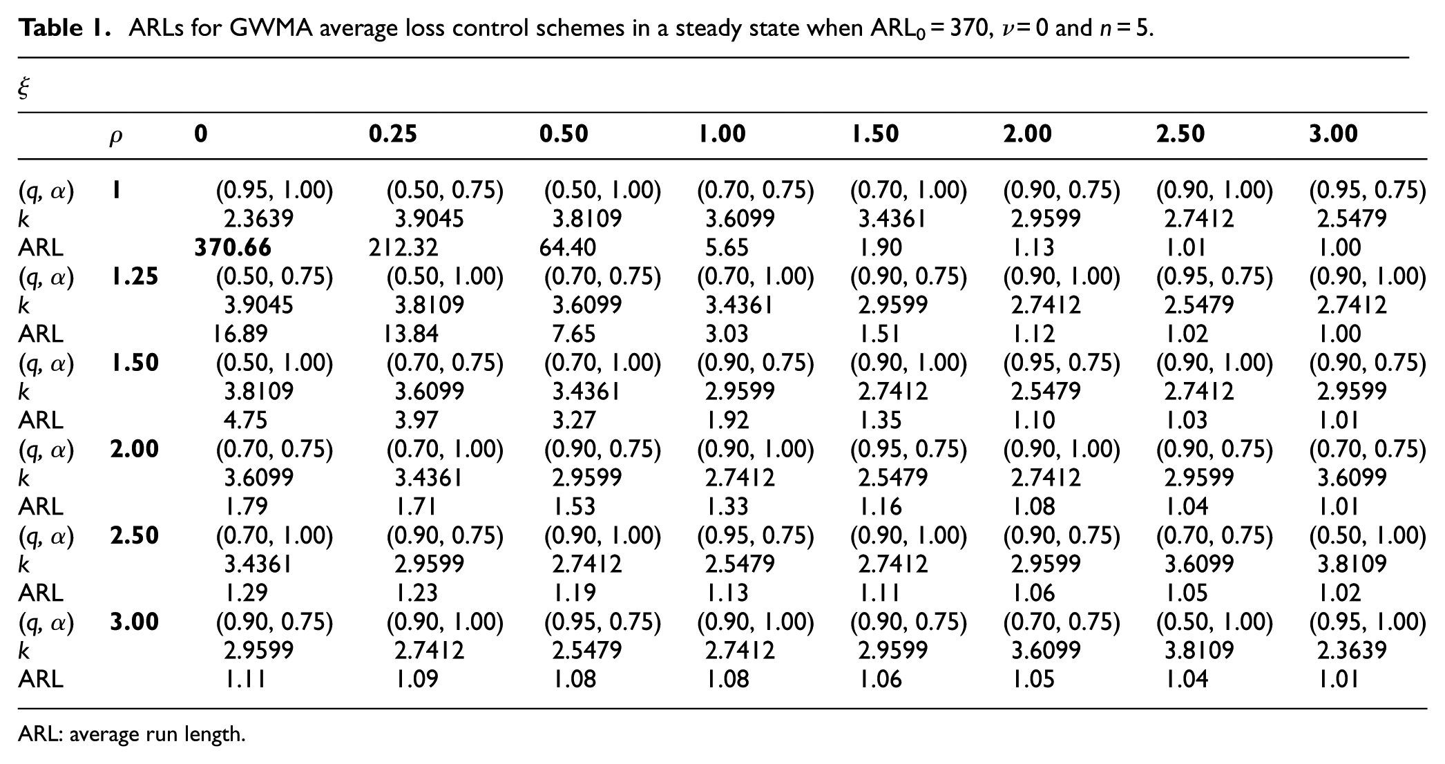
ARLs for GWMA average loss control schemes in a steady state when ARL₀ = 370, ν = 0 and n = 5.

ξ
	ρ	0	0.25	0.50	1.00	1.50	2.00	2.50	3.00
(q, α)	1	(0.95, 1.00)	(0.50, 0.75)	(0.50, 1.00)	(0.70, 0.75)	(0.70, 1.00)	(0.90, 0.75)	(0.90, 1.00)	(0.95, 0.75)
k		2.3639	3.9045	3.8109	3.6099	3.4361	2.9599	2.7412	2.5479
ARL		370.66	212.32	64.40	5.65	1.90	1.13	1.01	1.00
(q, α)	1.25	(0.50, 0.75)	(0.50, 1.00)	(0.70, 0.75)	(0.70, 1.00)	(0.90, 0.75)	(0.90, 1.00)	(0.95, 0.75)	(0.90, 1.00)
k		3.9045	3.8109	3.6099	3.4361	2.9599	2.7412	2.5479	2.7412
ARL		16.89	13.84	7.65	3.03	1.51	1.12	1.02	1.00
(q, α)	1.50	(0.50, 1.00)	(0.70, 0.75)	(0.70, 1.00)	(0.90, 0.75)	(0.90, 1.00)	(0.95, 0.75)	(0.90, 1.00)	(0.90, 0.75)
k		3.8109	3.6099	3.4361	2.9599	2.7412	2.5479	2.7412	2.9599
ARL		4.75	3.97	3.27	1.92	1.35	1.10	1.03	1.01
(q, α)	2.00	(0.70, 0.75)	(0.70, 1.00)	(0.90, 0.75)	(0.90, 1.00)	(0.95, 0.75)	(0.90, 1.00)	(0.90, 0.75)	(0.70, 0.75)
k		3.6099	3.4361	2.9599	2.7412	2.5479	2.7412	2.9599	3.6099
ARL		1.79	1.71	1.53	1.33	1.16	1.08	1.04	1.01
(q, α)	2.50	(0.70, 1.00)	(0.90, 0.75)	(0.90, 1.00)	(0.95, 0.75)	(0.90, 1.00)	(0.90, 0.75)	(0.70, 0.75)	(0.50, 1.00)
k		3.4361	2.9599	2.7412	2.5479	2.7412	2.9599	3.6099	3.8109
ARL		1.29	1.23	1.19	1.13	1.11	1.06	1.05	1.02
(q, α)	3.00	(0.90, 0.75)	(0.90, 1.00)	(0.95, 0.75)	(0.90, 1.00)	(0.90, 0.75)	(0.70, 0.75)	(0.50, 1.00)	(0.95, 1.00)
k		2.9599	2.7412	2.5479	2.7412	2.9599	3.6099	3.8109	2.3639
ARL		1.11	1.09	1.08	1.08	1.06	1.05	1.04	1.01

ARL: average run length.

Table 2.

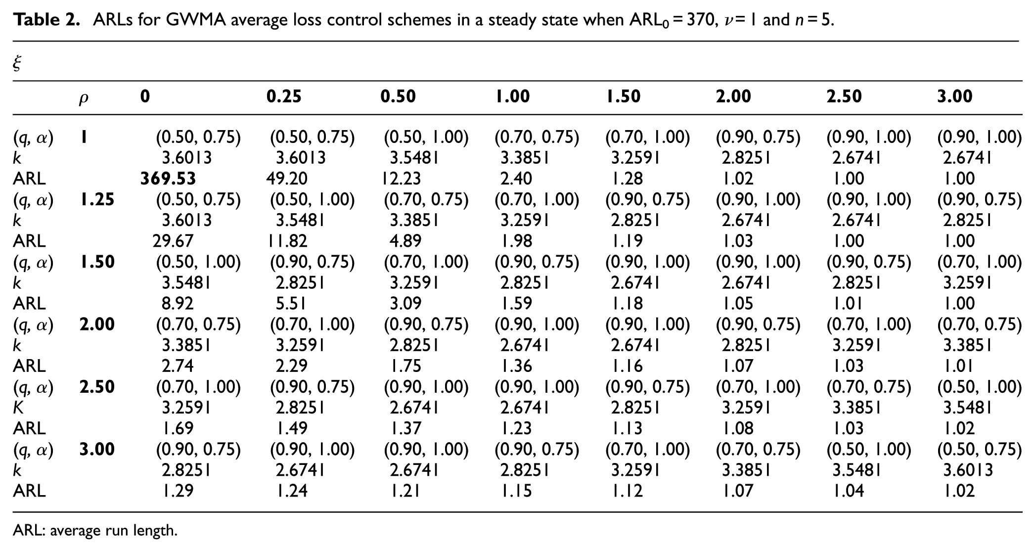
ARLs for GWMA average loss control schemes in a steady state when ARL₀ = 370, ν = 1 and n = 5.

ξ
	ρ	0	0.25	0.50	1.00	1.50	2.00	2.50	3.00
(q, α)	1	(0.50, 0.75)	(0.50, 0.75)	(0.50, 1.00)	(0.70, 0.75)	(0.70, 1.00)	(0.90, 0.75)	(0.90, 1.00)	(0.90, 1.00)
k		3.6013	3.6013	3.5481	3.3851	3.2591	2.8251	2.6741	2.6741
ARL		369.53	49.20	12.23	2.40	1.28	1.02	1.00	1.00
(q, α)	1.25	(0.50, 0.75)	(0.50, 1.00)	(0.70, 0.75)	(0.70, 1.00)	(0.90, 0.75)	(0.90, 1.00)	(0.90, 1.00)	(0.90, 0.75)
k		3.6013	3.5481	3.3851	3.2591	2.8251	2.6741	2.6741	2.8251
ARL		29.67	11.82	4.89	1.98	1.19	1.03	1.00	1.00
(q, α)	1.50	(0.50, 1.00)	(0.90, 0.75)	(0.70, 1.00)	(0.90, 0.75)	(0.90, 1.00)	(0.90, 1.00)	(0.90, 0.75)	(0.70, 1.00)
k		3.5481	2.8251	3.2591	2.8251	2.6741	2.6741	2.8251	3.2591
ARL		8.92	5.51	3.09	1.59	1.18	1.05	1.01	1.00
(q, α)	2.00	(0.70, 0.75)	(0.70, 1.00)	(0.90, 0.75)	(0.90, 1.00)	(0.90, 1.00)	(0.90, 0.75)	(0.70, 1.00)	(0.70, 0.75)
k		3.3851	3.2591	2.8251	2.6741	2.6741	2.8251	3.2591	3.3851
ARL		2.74	2.29	1.75	1.36	1.16	1.07	1.03	1.01
(q, α)	2.50	(0.70, 1.00)	(0.90, 0.75)	(0.90, 1.00)	(0.90, 1.00)	(0.90, 0.75)	(0.70, 1.00)	(0.70, 0.75)	(0.50, 1.00)
K		3.2591	2.8251	2.6741	2.6741	2.8251	3.2591	3.3851	3.5481
ARL		1.69	1.49	1.37	1.23	1.13	1.08	1.03	1.02
(q, α)	3.00	(0.90, 0.75)	(0.90, 1.00)	(0.90, 1.00)	(0.90, 0.75)	(0.70, 1.00)	(0.70, 0.75)	(0.50, 1.00)	(0.50, 0.75)
k		2.8251	2.6741	2.6741	2.8251	3.2591	3.3851	3.5481	3.6013
ARL		1.29	1.24	1.21	1.15	1.12	1.07	1.04	1.02

ARL: average run length.

Table 3.

ARLs for GWMA average loss control schemes in a steady state when ARL₀ = 370, ν = 2 and n = 5.

ξ
	ρ	0	0.25	0.50	1.00	1.50	2.00	2.50	3.00
(q, α)	1	(0.50, 0.75)	(0.50, 0.75)	(0.50, 1.00)	(0.70, 0.75)	(0.70, 1.00)	(0.90, 0.75)	(0.90, 1.00)	(0.90, 1.00)
k		3.2865	3.2865	3.2269	3.1145	3.0299	2.6785	2.5699	2.5699
ARL		371.35	41.31	9.96	2.24	1.25	1.02	1.00	1.00
(q, α)	1.25	(0.50, 0.75)	(0.50, 1.00)	(0.70, 0.75)	(0.70, 1.00)	(0.90, 0.75)	(0.90, 1.00)	(0.90, 1.00)	(0.90, 0.75)
k		3.2865	3.2269	3.1145	3.0299	2.6785	2.5699	2.5699	2.6785
ARL		42.47	13.17	4.96	1.96	1.21	1.03	1.00	1.00
(q, α)	1.50	(0.50, 1.00)	(0.70, 0.75)	(0.70, 1.00)	(0.90, 0.75)	(0.90, 1.00)	(0.90, 1.00)	(0.90, 0.75)	(0.70, 1.00)
k		3.2269	3.1145	3.0299	2.6785	2.5699	2.5699	2.6785	3.0299
ARL		14.01	6.05	3.55	1.67	1.19	1.05	1.01	1.00
(q, α)	2.00	(0.70, 0.75)	(0.70, 1.00)	(0.90, 0.75)	(0.90, 1.00)	(0.90, 1.00)	(0.90, 0.75)	(0.70, 1.00)	(0.70, 0.75)
k		3.1145	3.0299	2.6785	2.5699	2.5699	2.6785	3.0299	3.1145
ARL		4.31	3.09	2.14	1.50	1.20	1.08	1.04	1.01
(q, α)	2.50	(0.70, 1.00)	(0.90, 0.75)	(0.90, 1.00)	(0.90, 1.00)	(0.90, 0.75)	(0.70, 1.00)	(0.70, 0.75)	(0.50, 1.00)
K		3.0299	2.6785	2.5699	2.5699	2.6785	3.0299	3.1145	3.2269
ARL		2.51	1.95	1.69	1.37	1.20	1.11	1.05	1.02
(q, α)	3.00	(0.90, 0.75)	(0.90, 1.00)	(0.90, 1.00)	(0.90, 0.75)	(0.70, 1.00)	(0.70, 0.75)	(0.50, 1.00)	(0.50, 0.75)
k		2.6785	2.5699	2.5699	2.6785	3.0299	3.1145	3.2269	3.2865
ARL		1.74	1.58	1.45	1.28	1.20	1.11	1.06	1.03

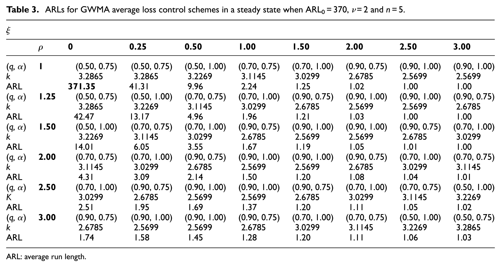
ARL: average run length.

These tables show the ARL₁s for different combinations of parameters (q = 0.50, 0.70, 0.90; α = 0.75, 1.00), which are used here when only the mean shifts (ρ = 1), only the variance shifts (ξ = 0) and when both the mean and variance shift together. Table 1 corresponds to the value of ν = 0 while Tables 2 and 3 correspond to ν = 1 and ν = 2, respectively, for the fixed sample size n = 5.

When ν = 0, a moderate change is observed in ARLs especially when only the mean shifts in the process, but a rapid decrease is observed when only the variance shifts and when both shift simultaneously. On the other hand, when ν = 1, 2, a quick decrease is not only detected in the variance and when both shift but also a rapid decrease is analyzed in the process mean. It is also evaluated that in order to detect a quick shift in the variance only, a small value of ν is recommended.

Sheu and Lin³³ observed that GWMA chart is more sensitive for a large value of q and when α lied between 0.50 and 1.00 when they first proposed GWMA control scheme. According to Lucas and Saccucci³⁸ and Roberts,²⁹ EWMA control scheme is more sensitive when a smaller value of λ is used, say 0 < λ ≤ 0.30.

The results revealed that this proposed GWMA control scheme is also more sensitive for a large value of q (say 0.70 ≤ q ≤ 1.00) and when α lied between 0.50 and 1.00, but somehow when ν ≠ 0, a moderate value of q provides quick out-of-control indication especially for the mean shift.

Table 4 shows a comparison between GWMA average loss chart and VSI EWMA and FP EWMA average loss charts proposed by Yang.²⁸ Yang²⁸ used different combinations for ξ (=0.5, 1.5, 2.5), ρ (=1.5, 2.0, 2.5) and ν (=0, 1, 2) to find ARL₁ for different levels of λ = .1, 0.3, 0.5 and the subgroup size n = 5 while choosing ARL₀ = 370. To compare GWMA average loss chart, we use α = 0.75, 1.00 and q = 0.9, 0.7, 0.5 and taking the same remaining parameters for ξ, ν and ρ, to find ARL₁ by setting ARL₀ = 370, and observed that GWMA average loss chart is more sensitive than FP EWMA average loss chart, but VSI EWMA loss chart has overall better performance than the proposed GWMA average loss chart. The reason for such a scenario is that GWMA average loss chart is evaluated with fixed sampling intervals and the VSI schemes have advantage over fixed sampling interval schemes.²⁸

Table 4.

Comparison of ARL₁s of GWMA average loss chart with FP EWMA.²⁸

ξ	ρ	ν	λ = 1 − q	k	VSI EWMA	FP EWMA	k^*	GWMA (α = 0.75)	k^*	GWMA (α = 1.00)
0.5	1.5	0	0.1	2.731	0.692	4.009	2.960	2.766	2.741	2.698
0.5	1.5	1	0.3	3.258	2.004	3.576	3.385	3.196	3.259	3.087
0.5	1.5	2	0.5	3.247	3.082	4.166	3.287	4.003	3.227	3.889
0.5	2	1	0.1	2.658	0.385	2.514	2.825	1.754	2.674	1.733
0.5	2	2	0.3	3.039	1.601	2.740	3.115	2.374	3.030	2.395
0.5	2	0	0.5	3.814	1.533	1.846	3.905	1.765	3.811	1.735
0.5	2.5	2	0.1	2.566	0.446	2.436	2.679	1.711	2.570	1.694
0.5	2.5	0	0.3	3.444	0.714	1.392	3.610	1.288	3.436	1.263
0.5	2.5	1	0.5	3.551	1.434	1.606	3.601	1.528	3.548	1.536
1.5	1.5	0	0.3	3.444	0.210	1.693	3.610	1.507	3.436	1.464
1.5	1.5	1	0.5	3.551	0.703	1.391	3.601	1.319	3.548	1.307
1.5	1.5	2	0.1	2.566	1.469	1.808	2.679	1.209	2.570	1.195
1.5	2	1	0.3	3.258	0.157	1.346	3.385	1.227	3.259	1.209
1.5	2	2	0.5	3.247	0.699	1.360	3.287	1.306	3.227	1.298
1.5	2	0	0.1	2.731	1.383	1.536	2.960	1.204	2.741	1.189
1.5	2.5	2	0.3	3.039	0.179	1.356	3.115	1.232	3.030	1.223
1.5	2.5	0	0.5	3.814	0.606	1.195	3.905	1.169	3.811	1.163
1.5	2.5	1	0.1	2.658	1.288	1.374	2.825	1.130	2.674	1.123
2.5	1.5	0	0.5	3.814	0.109	1.076	3.905	1.057	3.811	1.056
2.5	1.5	1	0.1	2.658	0.552	1.104	2.825	1.011	2.674	1.009
2.5	1.5	2	0.3	3.039	1.116	1.049	3.115	1.017	3.030	1.015
2.5	2	1	0.5	3.551	0.106	1.048	3.601	1.035	3.548	1.033
2.5	2	2	0.1	2.566	0.584	1.167	2.679	1.023	2.570	1.023
2.5	2	0	0.3	3.444	1.139	1.090	3.610	1.052	3.436	1.046
2.5	2.5	2	0.5	3.247	0.112	1.071	3.287	1.059	3.227	1.052
2.5	2.5	0	0.1	2.731	0.560	1.116	2.960	1.034	2.741	1.029
2.5	2.5	1	0.3	3.258	1.129	1.067	3.385	1.034	3.259	1.036

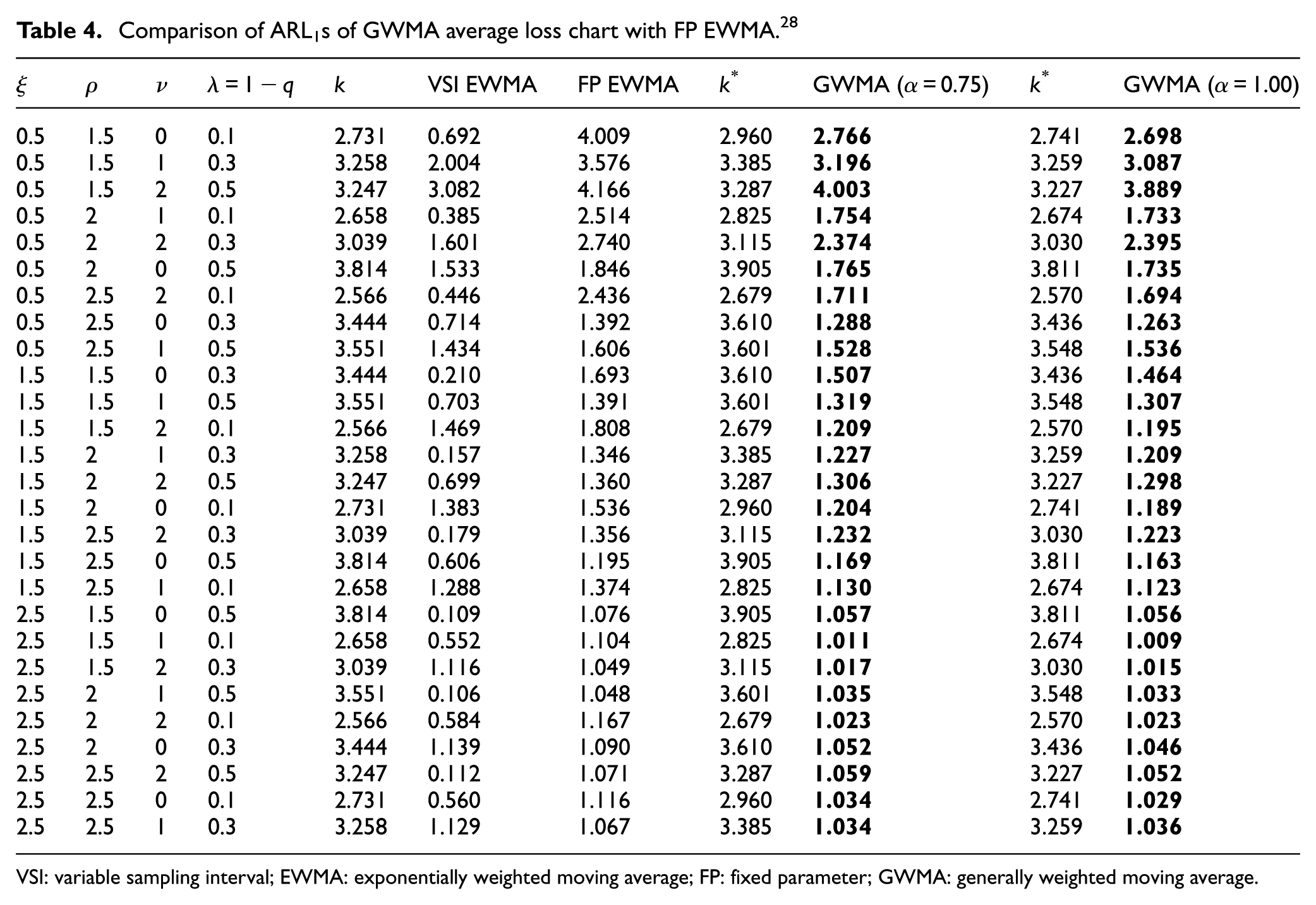
VSI: variable sampling interval; EWMA: exponentially weighted moving average; FP: fixed parameter; GWMA: generally weighted moving average.

ARL₁s calculated from this proposed chart are smaller than ARL₁s of Yang’s chart for all the combinations of parameters at both different levels of α. Also since for α = 1, this chart becomes FP EWMA average loss chart, so at the same level GWMA shows better performance as compared to FP EWMA average loss chart as highlighted in Table 4. (Here, control factor k^* is used for GWMA average loss chart.)

Another comparison is made of ARL₁s with EWMA-SC chart by Chen et al.¹⁸ for different values of (q, α) and λ at different shifts of µ and σ in Table 5. Chen et al.¹⁸ used ARL₀ = 370 and n = 5 to obtain optimal combinations of (λ, L), so optimal combinations of (q, α, k) are calculated at the same level of ARL₀ = 370 and n = 5 in this proposed chart. Shift in the standard deviation is represented in the row while shift in the mean is shown in the column. Clearly, it can be seen that GWMA average loss chart gives better alarm of out-of-control signal at different shifts than the existing chart as shown in bold in Table 5 which indicates the sensitivity of the proposed chart.

Table 5.

Comparison of ARL₁s of GWMA average loss control schemes in a steady state with EWMA-SC chart¹⁸ when ARL₀ = 370, ν = 0 and n = 5.

ξ
Chart		ρ	0	0.25	0.50	1.00	1.50	2.00	2.50	3.00
EWMA	λ	1.00	0.010	0.010	0.050	0.050	0.365	0.655	0.900	0.980
	L		1.5957	1.5957	1.9479	1.9479	3.5795	3.9958	4.1577	4.1428
	ARL₁		370.29	93.18	23.66	5.33	2.26	1.30	1.04	1.00
GWMA	ARL₁		370.08	91.11	22.33	3.58	2.03	1.28	1.04	1.00
	(q, α)		(0.99, 0.75)	(0.99, 0.75)	(0.95, 0.75)	(0.95, 0.75)	(0.635, 0.85)	(0.345, 0.70)	(0.10, 0.90)	(0.02, 0.75)
	k		1.9845	1.9845	2.5479	2.5479	3.6559	4.0379	4.1535	4.1595
EWMA	λ	1.25	0.050	0.050	0.050	0.265	0.465	0.675	0.885	0.975
	L		1.9479	1.9479	1.9479	3.3459	3.7551	4.0154	4.1528	4.1724
	ARL₁		9.80	8.80	6.73	3.47	1.89	1.27	1.06	1.01
GWMA	ARL₁		7.48	6.46	4.68	3.09	1.79	1.26	1.06	1.01
	(q, α)		(0.95, 0.75)	(0.95, 0.75)	(0.95, 0.75)	(0.735, 0.75)	(0.535, 0.80)	(0.325, 0.70)	(0.115, 0.80)	(0.025, 0.75)
	k		2.5479	2.5479	2.5479	3.5249	3.8476	4.0636	4.1419	4.1579
EWMA	λ	1.50	0.050	0.050	0.275	0.365	0.555	0.700	0.870	0.950
	L		1.9479	1.9479	3.3749	3.5795	3.8846	4.0392	4.1473	4.1708
	ARL₁		4.48	4.28	3.71	2.44	1.64	1.24	1.07	1.01
GWMA	ARL₁		2.97	2.84	2.76	2.22	1.61	1.22	1.07	1.01
	(q, α)		(0.95, 0.75)	(0.95, 0.75)	(0.90, 0.75)	(0.635, 0.85)	(0.445, 0.60)	(0.30, 0.90)	(0.13, 0.75)	(0.05, 0.65)
	k		2.5479	2.5479	2.9599	3.6559	4.0087	4.0499	4.1379	4.1553
EWMA	λ	2.00	0.465	0.465	0.485	0.555	0.655	0.785	0.880	0.950
	L		3.7551	3.7551	3.7880	3.8846	3.9958	4.1042	4.1511	4.1693
	ARL₁		1.96	1.93	1.84	1.58	1.33	1.16	1.07	1.03
GWMA	ARL₁		1.88	1.84	1.76	1.56	1.33	1.17	1.07	1.02
	(q, α)		(0.535, 0.80)	(0.535, 0.80)	(0.515, 0.80)	(0.445, 0.60)	(0.345, 0.70)	(0.215, 0.80)	(0.12, 0.85)	(0.05, 0.65)
	k		3.8476	3.8476	3.8639	4.0087	4.0379	4.1138	4.1436	4.1553
EWMA	λ	2.50	0.655	0.655	0.655	0.675	0.755	0.845	0.880	0.980
	L		3.9958	3.9958	3.9958	4.0154	4.0842	4.1363	4.1511	4.1655
	ARL₁		1.38	1.35	1.37	1.27	1.18	1.11	1.06	1.02
GWMA	ARL₁		1.36	1.35	1.34	1.26	1.18	1.11	1.06	1.02
	(q, α)		(0.345, 0.70)	(0.345, 0.70)	(0.345, 0.70)	(0.325, 0.70)	(0.245, 0.90)	(0.155, 0.75)	(0.12, 0.85)	(0.02, 0.75)
	k		4.0379	4.0379	4.0379	4.0636	4.0916	4.1388	4.1436	4.1595
EWMA	λ	3.00	0.775	0.785	0.785	0.815	0.845	0.880	0.930	0.930
	L		4.0978	4.1042	4.1042	4.1215	4.1363	4.1511	4.1655	4.1655
	ARL₁		1.18	1.17	1.17	1.14	1.10	1.07	1.04	1.02
GWMA	ARL₁		1.17	1.17	1.17	1.13	1.10	1.07	1.04	1.02
	(q, α)		(0.225, 0.75)	(0.215, 0.80)	(0.215, 0.80)	(0.185, 0.70)	(0.155, 0.75)	(0.12, 0.85)	(0.07, 0.65)	(0.07, 0.65)
	k		4.1120	4.1138	4.1138	4.1527	4.1388	4.1436	4.1533	4.1533

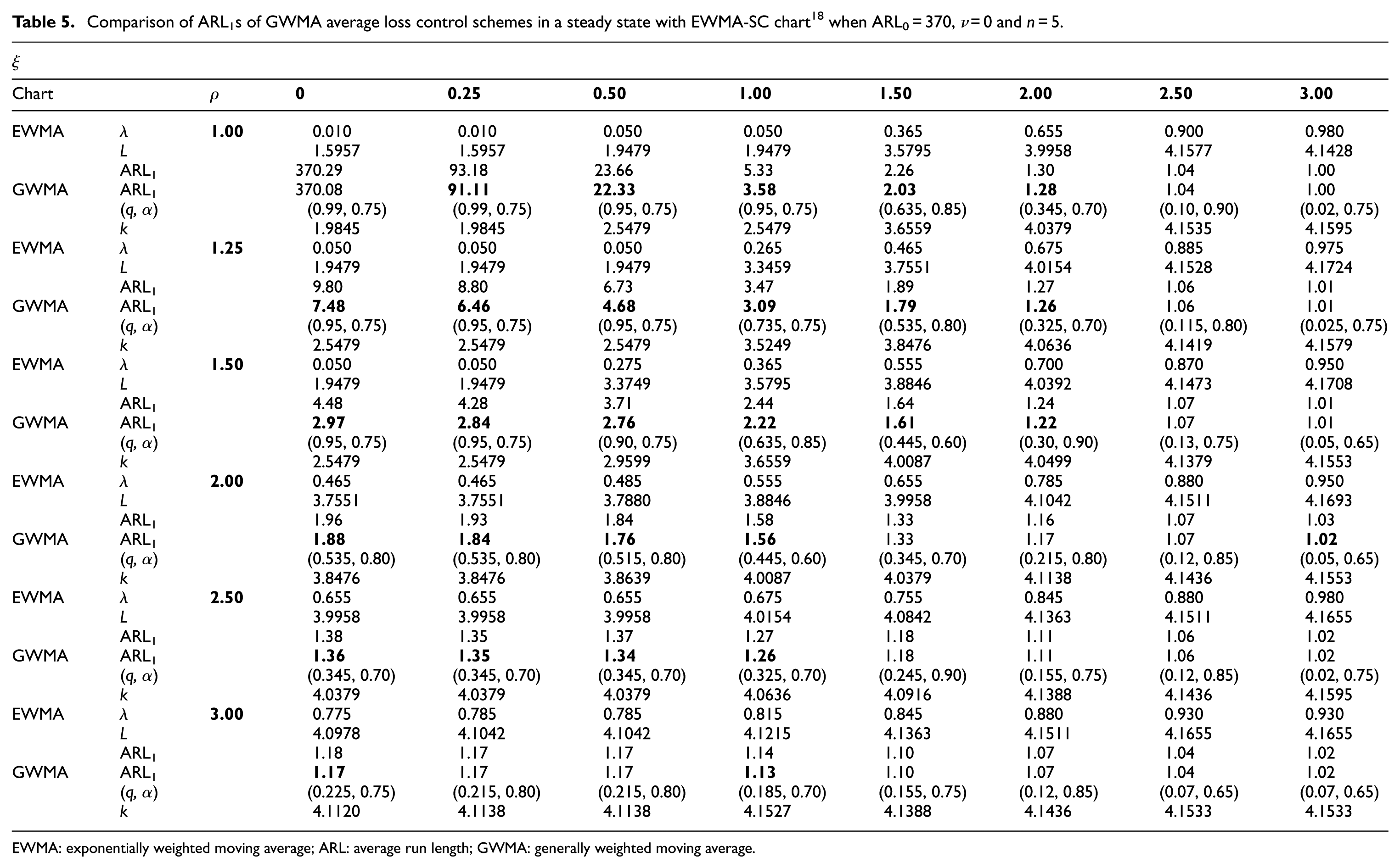
EWMA: exponentially weighted moving average; ARL: average run length; GWMA: generally weighted moving average.

The literature of GWMA charts such as by Sheu and Lin,³³ Sheu et al.,^22,24 Sheu and Hsieh⁸ and Teh et al.²⁵ shows that GWMA scheme has performed almost 60%–80% better than EWMA scheme. Tables 4 and 5 show that GWMA average loss chart is more efficient than the extended VSI EWMA average loss control chart²⁸ and EWMA-SC chart,¹⁸ especially for moderate shifts and almost 60% combinations of the shifts showed better overall performance.

Examples

This example is obtained from Chen et al.,¹⁸ where the data include 35 samples of size five representing the measurements of the inside diameter of cylinder bores in an engine block such as 3.5205, 3.5202 and so on 3.5204. For simplicity, the last three digits of the measurements are used in this example as shown in Table 6.

Table 6.

Cylinder diameter data.

Sample j	X ₁	X ₂	X ₃	X ₄	X ₅	U_j	UCL_GWMA
1	205	202	204	207	205	1.760	5.936
2	202	196	201	198	202	1.610	6.103
3	201	202	199	197	196	1.641	6.203
4	205	203	196	201	197	1.881	6.272
5	199	196	201	200	195	1.954	6.324
6	203	198	192	217	196	4.673	6.364
7	202	202	198	203	202	3.557	6.397
8	197	196	196	200	204	3.514	6.425
9	199	200	204	196	202	3.299	6.448
10	202	196	204	195	197	3.471	6.467
11	205	204	202	208	205	3.963	6.484
12	200	201	199	200	201	3.343	6.498
13	205	196	201	197	198	3.459	6.511
14	202	199	200	198	200	3.117	6.522
15	200	200	201	205	201	3.023	6.532
16	201	187	209	202	200	4.768	6.541
17	202	202	204	198	203	4.065	6.548
18	201	198	204	201	201	3.734	6.555
19	207	206	194	197	201	4.378	6.562
20	200	204	198	199	199	3.901	6.567
21	203	200	204	199	200	3.685	6.572
22	196	203	197	201	194	3.936	6.577
23	197	199	203	200	196	3.760	6.581
24	201	197	196	199	207	3.978	6.585
25	204	196	201	199	197	3.850	6.588
26	206	206	199	200	203	4.038	6.591
27	204	203	199	199	197	3.830	6.594
28	199	201	201	194	200	3.774	6.597
29	201	196	197	204	200	3.735	6.599
30	203	206	201	196	201	3.833	6.601
31	203	197	199	197	201	3.654	6.603
32	197	194	199	200	199	3.725	6.605
33	200	201	200	197	200	3.422	6.607
34	199	199	201	201	201	3.185	6.608
35	200	204	197	197	197	3.324	6.610

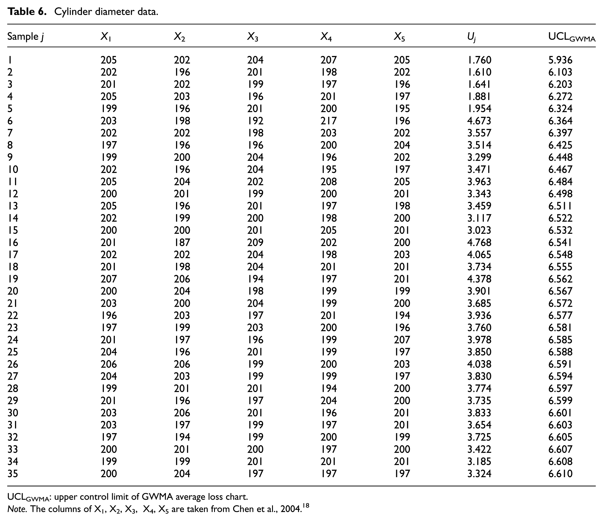
UCL_GWMA: upper control limit of GWMA average loss chart.

Note. The columns of X₁, X₂, X₃, X₄, X₅ are taken from Chen et al., 2004.¹⁸

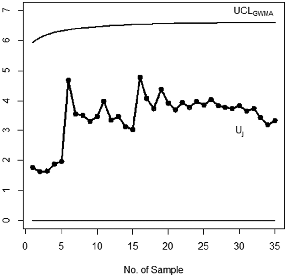
From the data in Table 6, we calculate $\bar{\bar{x}} = 200.24$ and ${\bar{S}}^{2} = 12.589$ as unbiased estimators of µ and σ², respectively, because both are unknown. The optimal combination of design parameters of the proposed chart (q, α, k) = (0.90, 0.75, 2.9599) is chosen to plot the cylinder diameter data in a steady state with in-control ARL = 370 from Table 1. In Table 6, U_j and upper control limit of GWMA average loss chart (UCL_GWMA) represent the statistic and upper control limit of GWMA average loss control chart, respectively, and the LCL is 0. In this example, we suppose that the target value T^* is equal to µ. Figure 1 shows the performance of GWMA average loss control chart for cylinder diameter data in a steady state.

Figure 1.

GWMA average loss chart.

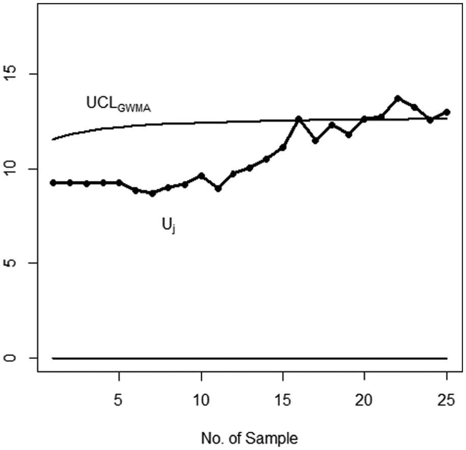
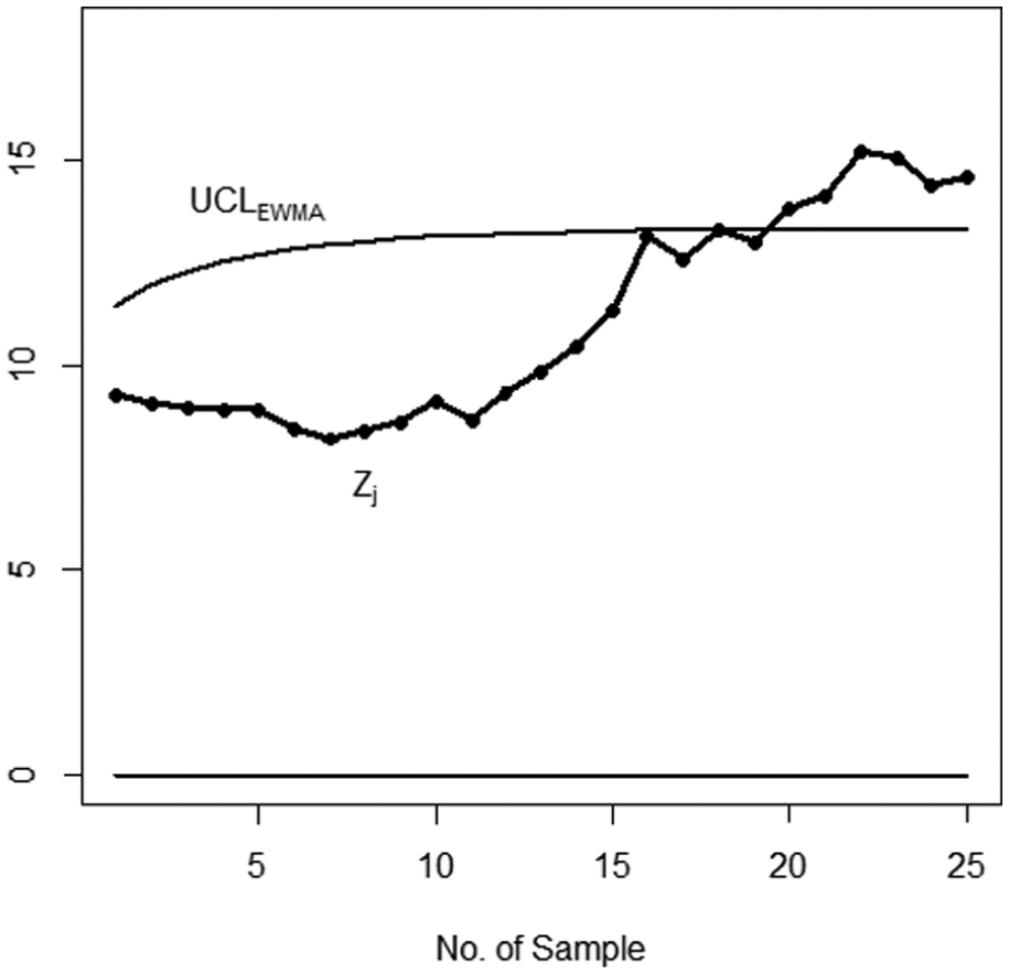
Another example is given in which simulated dataset is used to evaluate the performance of this proposed chart. In this example, 25 subgroups of size n = 5 are used where the first 10 subgroups are generated from in-control process with µ = 2, and σ = 1 and the remaining 15 subgroups are generated from an out-of-control process with a shift of 0.25σ and 1.50σ in the process mean and standard deviation, respectively, as shown in Table 7.

Table 7.

Simulated dataset from normal distribution having µ and σ².

Sample j	X ₁	X ₂	X ₃	X ₄	X ₅	Z_j	UCL_EWMA	U_j	UCL_GWMA
1	1.7431	1.6175	1.9712	0.4834	1.6315	9.254	11.456	9.254	11.547
2	1.8194	1.0009	1.2918	2.1894	3.3318	9.090	11.959	9.296	11.824
3	1.7636	3.0701	1.0615	1.7843	2.4650	8.944	12.286	9.233	11.988
4	3.4667	1.2790	1.9142	1.0875	2.2946	8.918	12.521	9.269	12.102
5	2.0338	2.3736	2.6044	2.5646	1.8775	8.901	12.695	9.273	12.188
6	2.0832	1.2367	−0.1940	0.3417	2.2122	8.466	12.829	8.848	12.255
7	0.4192	2.2980	1.3728	1.9828	2.6627	8.209	12.933	8.709	12.310
8	2.7356	1.1232	3.6887	0.9040	0.7676	8.420	13.015	9.009	12.355
9	1.6160	1.6724	1.7044	3.2822	2.9696	8.620	13.079	9.164	12.393
10	2.3616	3.7519	0.2780	1.5884	2.8821	9.141	13.130	9.619	12.425
11	1.3114	0.1012	2.7078	0.7288	1.4882	8.641	13.171	8.952	12.453
12	1.7725	0.6261	3.6650	3.6638	1.8225	9.338	13.204	9.745	12.477
13	3.3307	3.3317	1.8377	0.0926	2.4319	9.848	13.230	10.065	12.498
14	0.8883	−0.1487	0.4603	1.3568	4.7904	10.475	13.251	10.509	12.516
15	0.8795	2.0165	4.1453	2.5152	3.4414	11.347	13.268	11.160	12.532
16	5.5067	3.3718	0.8198	−0.0178	2.4644	13.128	13.282	12.645	12.547
17	2.2230	2.6975	0.6569	0.3302	2.5851	12.560	13.293	11.518	12.560
18	1.4245	4.0103	3.9328	1.6872	−0.3822	13.327	13.302	12.325	12.571
19	1.9952	3.2933	0.4883	1.8267	2.7343	13.015	13.309	11.789	12.582
20	2.4774	2.8475	1.6476	4.3534	2.9875	13.834	13.315	12.658	12.591
21	1.1316	2.5925	1.3989	0.0268	4.5951	14.109	13.320	12.719	12.599
22	0.5011	4.2876	2.0552	3.8118	3.2638	15.218	13.324	13.730	12.607
23	1.2147	1.7098	3.2539	1.5608	3.7825	15.065	13.327	13.264	12.614
24	2.9763	2.5045	2.0591	1.8546	1.5148	14.387	13.329	12.589	12.620
25	3.5218	2.3184	2.1358	3.0466	2.7657	14.618	13.331	13.021	12.625

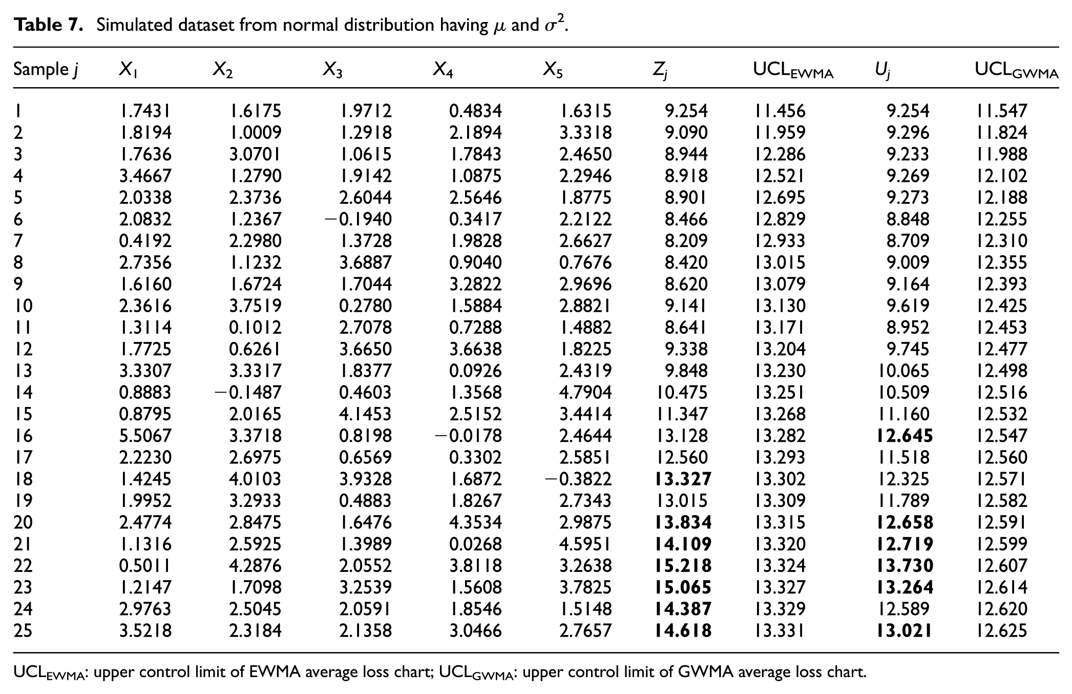
UCL_EWMA: upper control limit of EWMA average loss chart; UCL_GWMA: upper control limit of GWMA average loss chart.

In this example, target value T^* is supposed to be 1, that is, T^* = 1 then the value of ν becomes 1 such that ν = 1. From Table 2, the optimal combinations of (λ, k) = (0.10, 2.658) and (q, α, k) = (0.90, 0.75, 2.825) are chosen for EWMA and GWMA average loss charts, respectively, when ARL₀ = 370.

In this case, when T^* is not equal to µ, we can see from Figures 2 and 3 that GWMA average loss chart detects first out-control signal at 16th sample while EWMA average loss chart detects first out of signal at 18th sample, as highlighted in Table 7. It shows that GWMA average loss chart detects the out-of-control process signal prior to the EWMA average loss chart which indicates the performance of proposed chart for detecting small shifts occurred in the process.

Figure 2.

GWMA average loss chart.

Figure 3.

EWMA average loss chart.

Conclusion

GWMA average loss chart is designed to detect small shifts in the process mean or standard deviation or both using the Taguchi loss function. GWMA average loss chart shows better overall performance than FP EWMA average loss chart²⁷ and EWMA-SC chart.¹⁸ Two practical examples are included: one from real data and one from simulated data, to clarify the performance of the chart. Since its computation is difficult as compared to EWMA chart, but in today’s modern technology it is not a matter of worry. This chart can widely be used in the industries where the manufacturing process is observed.

Footnotes

Appendix 1 Acknowledgements

The authors are deeply thankful to the editor and the reviewers for their valuable suggestions to improve the quality of this article. M.A., therefore, acknowledges with thanks DSR for the technical support.

Declaration of Conflicting Interests

The author(s) declared no potential conflicts of interest with respect to the research, authorship and/or publication of this article.

Funding

The author(s) disclosed receipt of the following financial support for the research, authorship, and/or publication of this article: This article was funded by the Deanship of Scientific Research (DSR), King Abdulaziz University, Jeddah.

References

Aslam

Khan

Jun

CH.

A new S2 control chart using repetitive sampling. J Appl Stat 2015; 42(11): 2485–2496.

Aslam

Azam

Jun

CH.

New attributes and variables control charts under repetitive sampling. Ind Eng Manag Syst 2014; 13(1): 101–106.

Azam

Aslam

Jun

. Designing of a hybrid exponentially weighted moving average control chart using repetitive sampling. Int J Adv Manuf Tech 2015; 77(9): 1927–1933.

Haq

Brown

Moltchanova

New exponentially weighted moving average control charts for monitoring process dispersion. Qual Reliab Eng Int 2014; 30: 1311–1332.

Huang

Chen

Sheu

. Enhancement of axle bearing quality in sewing machines using Six Sigma. Proc IMechE, Part B: J Engineering Manufacture 2010; 224: 1581–1590.

Huwang

Huang

Wang

YHT

. New EWMA control charts for monitoring process dispersion. Comput Stat Data An 2010; 54: 2328–2342.

Lee

. An adaptive CUSUM chart with single sample size for monitoring process mean and variance. Qual Reliab Eng Int 2012; 29: 1027–1039.

Sheu

Hsieh

YT.

The extended GWMA control chart. J Appl Stat 2009; 36(2): 135–147.

Montgomery

DC.

Introduction to statistical quality control. 6th ed.New York: John Wiley & Sons, Inc., 2009.

10.

Ahmad

Aslam

Jun

CH.

Designing of X-bar control charts based on process capability index using repetitive sampling. T I Meas Control 2014; 36(3): 367–374.

11.

Al-Refaie

MHC

Chang

. Application of the Taguchi approach to improve performance of the alignment-layer printing process in liquid crystal displays. Proc IMechE, Part B: J Engineering Manufacture 2012; 226(7): 1241–1248.

12.

Aslam

Azam

Jun

. A new control chart for exponential distributed life using EWMA. T I Meas Control 2015; 37(2): 205–210.

13.

Castagliola

Vannman

Monitoring capability indices using an EWMA approach. Qual Reliab Eng Int 2007; 23: 769–790.

14.

Khoo

MBC

Teoh

Castagliola

. Optimal designs of the double sampling X-bar chart with estimated parameters. Int J Prod Econ 2013; 144: 345–357.

15.

Ouyang

Hsu

Yang

CM.

A new process capability analysis chart approach on the chip resistor quality management. Proc IMechE, Part B: J Engineering Manufacture 2013; 227(7): 1075–1082.

16.

Yeong

Khoo

MBC

Lee

. Economic and economic statistical designs of the synthetic X chart using loss functions. Eur J Oper Res 2013; 228: 571–581.

17.

Chen

Cheng

Xie

Monitoring process mean and variability with one EWMA chart. J Qual Technol 2001; 33(2): 223–233.

18.

Chen

Cheng

Xie

A new EWMA control chart for monitoring both location and dispersion. Qual Technol Quant Manag 2004; 1(2): 217–231.

19.

Tian

Weighted-loss-function CUSUM chart for monitoring mean and variance of a production process. Int J Prod Res 2005; 43(14): 3027–3044.

20.

Tian

Weighted-loss-function control charts. Int J Adv Manuf Tech 2006; 31: 107–115.

21.

Jiao

Helo

PT.

Optimization design of a CUSUM control chart based on Taguchi’s loss function. Int J Adv Manuf Tech 2008; 35: 1234–1243.

22.

Sheu

Tai

Hsieh

. Monitoring process mean and variability with generally weighted moving average control charts. Comput Ind Eng 2009; 57: 401–407.

23.

Teh

Khoo

MBC

A sum of squares double EWMA chart. Comput Ind Eng 2011; 61: 1173–1188.

24.

Sheu

Huang

Hsu

TS.

Extended maximum generally weighted moving average control chart for monitoring process mean and variability. Comput Ind Eng 2012; 62: 216–225.

25.

Teh

Khoo

MBC

Monitoring process mean and variance with a single generally weighted moving average chart. Commun Stat Theo Method 2012; 41(12): 2221–2241.

26.

Yang

Lee

. The X control chart for monitoring process shifts in mean and variance. Int J Prod Res 2012; 50(3): 893–907.

27.

Yang

SF.

Using a single average loss control chart to monitor process mean and variability. Commun Stat Simulat 2013; 42(7): 1549–1562.

28.

Yang

SF.

Using a new VSI EWMA average loss control chart to monitor changes in the difference between the process mean and target and/or the process variability. Appl Math Model 2013; 37: 7973–7982.

29.

Roberts

SW.

Control chart tests based on geometric moving averages. Technometrics 1959; 42(1): 97–101.

30.

Sheu

Griffith

WS.

Optimal number of minimal repairs before replacement of a system subject to shocks. Nav Res Log 1996; 43: 319–333.

31.

Sheu

SH.

A generalized age and block replacement of a system subject to shocks. Eur J Oper Res 1998; 108: 345–362.

32.

Sheu

SH.

Extended optimal replacement model for deteriorating systems. Eur J Oper Res 1999; 112: 503–516.

33.

Sheu

Lin

TC.

The generally weighted moving average control chart for detecting small shifts in the process mean. Qual Eng 2003; 16(2): 209–231.

34.

Trietsch

Statistical quality control. Singapore: World Scientific Publishing Co. Pte Ltd, 1999.

35.

Daya

Duffuaa

SO.

Integration of Taguchi’s loss function approach in the economic design of x-bar chart. Int J Qual Reliab Manag 2003; 20(5): 607–619.

36.

Taguchi

Elsayed

Hsiang

Quality engineering in production systems. New York: McGraw-Hill, 1989.

37.

Chandra

MJ.

Statistical quality control. Boca Raton, FL: CRC Press LLC, 2001.

38.

Lucas

Saccucci

MS.

Exponentially weighted moving average control schemes: properties and enhancements. Technometrics 1990; 32(1): 1–12.

A new generally weighted moving average control chart based on Taguchi’s loss function to monitor process mean and dispersion

Abstract

Keywords

Introduction

Design of GWMA control chart using Taguchi loss function

Taguchi loss function

GWMA of Taguchi loss

Proposed control chart based on GWMA of Taguchi loss

Performance and evaluation

Examples

Conclusion

Footnotes

Appendix 1

Acknowledgements

Declaration of Conflicting Interests

Funding

References