Sage Journals: Discover world-class research

Abstract

This article demonstrates implementation of immersed boundary method in continuous casting simulation involving boundary movement. In this methodology, the immersed boundary method is coupled with the second-order accurate finite difference solution of unsteady three-dimensional heat conduction equation. The moving molten metal front is modelled using the immersed boundary method in a Cartesian mesh framework that provides simplicity in its implementation and reduces the computational time as compared to the adaptive mesh solutions. A parallel programming paradigm using message passing interface has been implemented to obtain enhanced computational efficiency. This study has focused on capturing moving boundary during continuous casting and predicts the temperature distribution and shell thickness under different cooling ambiences and casting function. Good agreements with published data and correlations are obtained through numerical analysis. Mould-region shell thickness agrees well with Chipman–Fondersmith correlations. A new correlation has been further proposed for the delay constant at different heat extraction rates. The effects of key parameters like casting speed, convection and radiation from the continuous casting are also quantified in attempt to avail the data for optimal design of continuous caster.

Keywords

Continuous casting numerical simulation immersed boundary method solidified shell thickness heat extraction casting speed

Introduction

Thermal transport phenomenon plays an important role in many manufacturing processes, and several experimental/numerical studies have been aimed to understand the thermal physics involved in these processes.^1,2 Continuous casting is one of the heavily practiced metallurgical processes where thermal transport phenomenon plays a significant role. It has an edge over other conventional casting practices due to several factors like simplicity, higher productivity, eco-friendliness, lower operating cost and wide applicabilities in product manufacturing at industrial scales. In this process, superheated liquid metal is fed into water-cooled mould along the gravity from which it is withdrawn continuously in order to have partially solidified billet, bloom or slab, which are further processed in rolling mills. Electromagnetic stirrer is also present to facilitate stirring process. It helps in achieving better homogeneity and properties of casting product.^2–6

During continuous casting process, superheated molten metal flows from the tudnish to the primary zone through meniscus and then to the secondary zone in order to obtain fully solidified state under controlled cooling ambiences. Superheat, as well as the latent heat, is extracted from the liquid regime while sensible heat is extracted from the solid regime. The primary section in the casting consists of water-cooled mould. Sets of nozzle are provided in the secondary section to spray water-mist on the upcoming strand. After this, there is a subzone for radiation cooling. These three zones appear in longitudinal succession along the length of the casting strand. Electromagnetic stirrers are present at different locations along the length of the casting. Depending upon the location, the electromagnetic stirrers are classified as mould, strand or end-electromagnetic stirrers. It also helps in maintaining the hyperbolic shape of solidification front due to the presence of magnetic field.^4,7 It provides intensive flow of molten metal inside the mould and thus assists in better exchange of heat between the surface and the interior of the casting product. This is due to the fact that the stirring is done using an inductor, which produces magnetic field and helps in setting eddy currents across the metal pool. In effect, Lorentz force is obtained, which helps in the movement of the liquid metal to the core of the strand.⁵ The stirrer prevents sticking of casting strand to the mould surface (which may lead to breakout). Moffatt⁴ showed that application of electromagnetic stirrer results in better surface finish of the casting product. Furthermore, it also helps in controlling the growth of dendritic microstructures during solidification.⁸ Nozzles in the secondary zone spray air–water mist on the surface of the out-coming casting strand. In the radiation zone, ambient still air is the sole cooling medium. At the starting of the process, a dummy bar is horizontally held at the end to restrain molten metal from spilling. It is removed once complete solidification is achieved in its vicinity. A general schematic diagram shows the arrangements of these different zones along a continuous caster (Figure 1).

Figure 1.

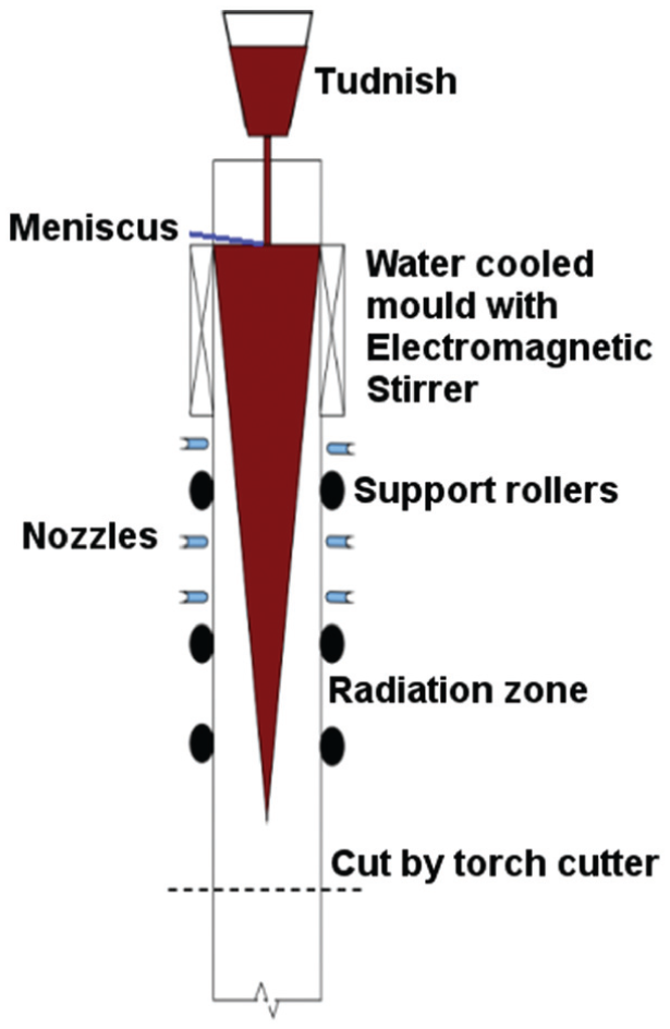
Schematic diagram of continuous casting process.

The casting process parameters are designed to obtain a sufficient solidified shell thickness at the primary zone, which should be able to deter the bursting phenomenon (a phenomenon in which the liquid molten metal comes out of surface below the exit of the mould). Occurrence of aforesaid phenomenon halts the continuity, and it becomes inevitable to restart the process from the beginning. Restarting the process is time consuming and results in wastage of molten raw materials, and thus increases the cost of production. Hence, the physics of metal flow in the primary zone has a very important role in the success of continuous casting process as well as in the quality of output products.

In the field of continuous casting, over several years, attempts have been made to develop this understanding in order to avoid surface defects, turnarounds and other defects. Rates of heat extraction from different sections of the cooling zones are of interest due to their influences in directional solidification and effects in the grain structures of the final product. Heat transfer rates can be obtained through analysis of the temperature profiles obtained for different arrangements of cooling section, dimension of cross section, rate of molten metal flow and intensive flow of metal due to electromagnetic stirrer. With the help of a priori information about the cooling parameters, the height of the mould can be determined which can sustain bursting (sufficient solidified shell thickness to balance ferrostatic pressure posed by molten metal). The other important parameters are length of secondary zone, radiation zone, sets of nozzle required in cooling zone, flow rate of water flow from nozzles and rate of molten metal flow in mould. Better understanding of the thermal physics of continuous casting process can help to build a pool of information on the effects of these parameters and finally to specify the optimal design of the process.

Several numerical models have been developed with respect to one-dimensional (1D),^9–11 two-dimensional (2D)^12–15 and three-dimensional (3D)^16,17 steady and transient assumptions in order to predict the temperature distribution, heat fluxes and solidification patterns. Researchers have used the finite element method,¹⁶ inverse finite element method,¹⁸ finite difference method,^{10,12,13,15,16,19} finite volume method¹⁴ and boundary element method²⁰ to solve numerically. The first few solidification models were based on 1D energy equation. Mizikar⁹ utilized 1D model to predict the thermal field and shell growth. Brimacombe¹⁰ predicted shell thickness and initial crack location using the finite difference scheme and further studied effects of reheating in continuous casting. Lally et al.¹² used 2D slices to model 3D steady-state temperature fields during continuous casting. Meng and Thomas¹³ performed heat transfer simulation in the mould as well as in the spray zone. Their model coupled 1D transient calculation of heat conduction within the solidifying steel shell with 2D steady-state heat conduction through the mould wall. They also considered air gap between the mould and solidified shell due to shrinkage of casting strand, effect of oscillation marks and mass and momentum balances at phase interface. Boehmer et al.¹⁹ studied the thermo-mechanical behaviour in continuous casting at high temperature and its effect on casting product using the finite difference method. They inferred that if effect of casting parameters is known a priori, then optimal casting condition could be addressed and hence able to avoid thermal cracking. Li and Thomas¹¹ proposed transient heat transfer model for single roll continuous strip casting process. Heat transfer through rotating wheel was also considered in their work. Tieu and Kim¹⁶ performed 3D simulation to get thermal field and determined shell thickness for multi-zonal cooling ambiences. Janik and Dyja¹⁷ used 3D energy equation to solve temperature field using the finite element method (ANSYS). Shell thickness and heat flux inside the mould were determined from the temperature distribution. Alizedeh et al.¹⁴ also utilized temperature field to predict shell thickness, interfacial gap between shell and mould and liquid pool positioning. They used a coordinate transformation technique to model the billet movement.

As continuous casting involves change of phases, it is important to track the interface between the molten and solidified phase. Siegel²¹ did extensive work on studying the interface behaviour during continuous casting and showed that its shape depends upon a single dimensionless parameter, which is function of casting velocity, the boundary conditions at the surface (cooling conditions) and width of the ingot. Malamataris and Papanastasiou¹⁸ proposed an empirical correlation for the shape of solidification front in terms of process parameters. They extended inverse isotherm finite element method to consider distorted isotherms. They also analysed high-speed continuous casting utilizing energy equation. Majchrzak²⁰ utilized boundary element method to trace the solidification front and obtain thermal field during continuous casting in order to predict temperature pattern across the billet. Das and Sarkar²² proposed a prediction model to predict the thermal profile during continuous casting using a coordinate transfer technique in a non-orthogonal control volume framework. This model involves tracking of the solid-liquid interface. A meshless method is also used to study the thermo-physics of pure metals during continuous casting method.²³ These approaches demand high computational time and complexity as it involves grid generation/mesh deformation at each time step to model the moving boundary.

Review of the literature (referred earlier in this section) reveals that for the study of thermal physics of continuous casting, different analysis approaches have been utilized. In broad way, these approaches could be categorized as follows:

On the basis of how energy equation is implemented in the considered domain:

Single region: ingle energy transport equation is considered for the entire casting irrespective of phase;

Multi-phase region: Energy transport equation is separately specified for each phase. Boundary conditions are imposed at interface through heat balance equation.

On the basis, how moving boundary problem (lower plate movement) is formulated:

By transforming the governing equation in a moving reference frame;

By simulating the boundary movement using dynamic grid generation.

Earlier works established that numerical simulations could be an effective tool to augment the detailed knowledge of different manufacturing processes (e.g. die-casting, investment casting, welding and friction stir welding (FSW)).^2,24,25 Recently, Soe²⁶ demonstrated that commercial softwares can be useful for accurate simulations of manufacturing processes and identify the important input parameters for optimization studies. Song and Kovacevic²⁵ also showed that for a manufacturing process like FSW, 3D transient heat transfer models can well predict the temperature variation during welding. Furthermore, numerical simulation has an edge over experimental approaches as it saves the material, time, money, energy and helps in building a pool of data for different materials along with the different process parameters. But, most of time, these manufacturing processes are involved with complex and moving geometries. Hence, they pose substantial challenges in boundary treatment while solving by traditional body conformal grid approaches. In contrast, immersed boundary method (IBM) (a non-conforming boundary approach)²⁷ has an edge over the boundary conforming grid. Here, as it offers much simplicity and computational efficiency in handling the moving boundary cases. In addition, immersed boundary (IB) also favours parallel paradigm without an increase in complexity.

IB method was first coined by Peskin,²⁷ who used this to simulate cardio-vascular flow problems. Most important feature of this method is that the entire simulation can be performed in the background of a Cartesian grid, which does not aligned with the complex geometry of the moving/fixed boundary, while the replication of boundary condition is achieved by imposing appropriate forcing term in the governing equation. This method needs an efficient algorithm to find the near-boundary mesh points where the interpolated values are to be specified. Simplicity and computational efficiency of IB methods have been discussed in a number of earlier published reports.^28–30 The advantages arise mainly due to the following facts: (a) costly body-fitted mesh generation can be avoided for complex geometry; (b) in body-fitted mesh approach using non-rectilinear meshes, calculation of metric quantities and flux variables are computationally involved, which is absolutely not needed in IB and (c) for moving geometry, re-meshing and mapping of older solutions to new meshes after each computational time step is not required. Computational efficiencies of IBM schemes were demonstrated by Verzicco et al.³¹ They reported that simulation time was much less in IBM than a coarser body-fitted mesh simulation³² for flow in a piston-cylinder arrangement with piston movement. Tyagi and Acharya³³ utilized IB method for large eddy simulation (LES) of turbulent flow in complex geometries. Their work also demonstrated different strategies for implementation of the forcing function. Mittal and Iaccarino³⁴ extensively studied different methods of IB implementation for immersed solid boundaries and shows its applicability over wide range of flow problems (such as flow past sphere and flapping wing). Heat transfer through complex and moving boundaries has been predicted by several researchers using IB methods.³⁵ Fadlun et al.³⁶ utilized IB method to study behaviour of fluid flow past complex geometry and reported the second-order accuracy in their results.

In this article, finite difference method for the 3D transient heat equation along with the IBM^27,34 has been used to predict the temperature profile and solidification pattern under multi-zonal cooling ambiences for continuous casting of steel alloy. A single region approach is used, which considered different phases of the steel alloy associated with respective thermal properties. For the mixed phase, the property values are interpolated at the local temperature using the solidus and liquidus properties. The moving boundary is modelled using a second-order accurate IB interpolation in a fixed coordinate system. The proposed methodology is simple to implement and moreover can be easily translated to parallel programming paradigm. This method further claims its applicability due to higher computational efficiency.^37,38 Solidification patterns are predicted for multi-cooling ambiences and effects of different casting parameters are studied.

Methodology

Problem formulation

The whole domain is considered as single region. 3D unsteady state heat conduction in Cartesian framework (equation (1)) is considered as governing equation for predicting the temperature profile of casting strand of alloys

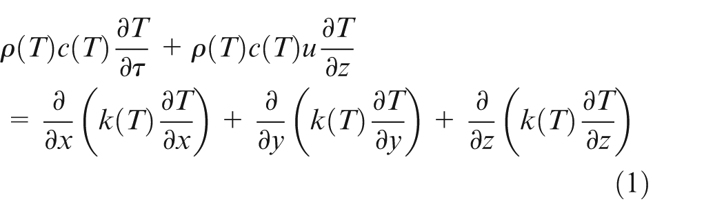
\begin{array}{l} ρ (T) c (T) \frac{\partial T}{\partial τ} + ρ (T) c (T) u \frac{\partial T}{\partial z} \\ = \frac{\partial}{\partial x} (k (T) \frac{\partial T}{\partial x}) + \frac{\partial}{\partial y} (k (T) \frac{\partial T}{\partial y}) + \frac{\partial}{\partial z} (k (T) \frac{\partial T}{\partial z}) \end{array}

(1)

Due to pouring and electromagnetic stirring effects, flow near the mould zone shows turbulent behaviour (Re: 10⁴–10⁵) leading to higher heat transfer. However, this article attempts to maintain the simplicity of the equation (1) without incorporating turbulence models into it and thus reduces the costs of computation. In earlier works, the effects of heat transfer augmentation due to turbulence have been mimicked by assigning a higher equivalent value of conductivity at the liquid and mushy zones.^9,39,40 The effective thermal conductivity can be four to eight times higher than its thermal conductivity of solid phase.^9,10 The idea of using higher equivalent k for liquid is first given by Mizikar⁹ to accommodate the effect of fluid motion and turbulence heat transfer. Till date, the higher conductivity modelling has widely been applied by many authors who envisaged the continuous casting phenomena. Saraswat et al.⁴¹ also showed that for a steel alloy, an effective higher thermal conductivity 5–15 times greater than the solid thermal conductivity predicts the solidification thickness within a range of 10% error as compared to k-epsilon model. However, it was established by Choudhary and Mazumdar⁴² that the predicted shell thickness depends on the values of equivalent conductivity (k). They also showed that better agreement with experimental result is obtained when a conjugate heat and flow simulation is performed. It is to be noted that all equivalent k approaches have completely ignored the convective effect due to motion of the bulk of molten/solidified metal during the entire continuous casting process. In this case, a partial k approach is used, where the equivalent k is considered only for turbulence due to electromagnetic stirrer (predominant in the mould zone liquid and mushy phase) while heat transfer due to bulk convection of the metal (both liquid and solidified) is taken care by a convective term. Our proposed model has reduced the dependency on higher equivalent k (choosing an equivalent k value in the range of 5–15 times of solid phase conductivity) as used in previous studies.^{9,10,17,39,43} A lower value of equivalent k (∼2–3 times of solid phase conductivity) has been considered in order to model the augmented heat transfer rates due to pouring, stirring and movement effects along with the convective heat transfer term (second-term in the right-hand side (RHS) of equation (1)). This formulation avoided solving expensive fluid momentum equations for the turbulent electromagnetic stirred mould region and reduced computational expenses.

Latent heat

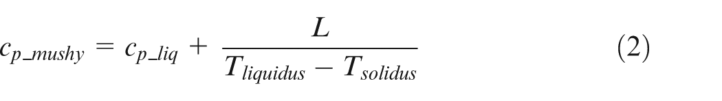
The latent heat of solidification can be considered by adding an enthalpy term in the governing equation (1) or by defining a specific scheme for increase in temperature for the mushy zone. The released fraction of latent heat in this regime is a function of the solid fraction.⁴⁴ Linear relationship can be used to calculate the equivalent specific heat during mushy zone. The equivalent specific heat for mushy zone is given by equation (2) as alloys have different liquidus and solidus temperature

c_{p_mushy} = c_{p_liq} + \frac{L}{T_{liquidus} - T_{solidus}}

(2)

Density

Generally, density is a function of temperature but the rate of change of density in relation with temperature for steel alloys is small due to lower values of thermal expansion coefficient suggesting a piece-wise continuous distribution over different phases. However, three distinctive densities have been considered respectively for the liquid, mushy and solid states.

Thermal conductivity

Thermal conductivity is modelled as linear function of temperature. In this case, a convection term in the direction of flow (casting speed, u) has been considered, whereas the effects of turbulent velocity and heat transfer in the horizontal plane are modelled using an equivalent higher thermal conductivity. The effect of turbulence and stirred whirls are dominant in the liquid and mushy phase and negligible in solid phase. Hence, higher value of equivalent thermal conductivity is considered in the near-mould regime where the effect of electromagnetic stirring is dominant.

Moving boundary modelling using IBM

During continuous casting, the molten metal flows as the lower boundary (or lower plate) moves and the casting grows in size. In order to utilize the simplicity of IBM, simulation is performed on the background of a fixed rectilinear mesh. For ease of implementation, the lower boundary is kept at a constant height and the upper boundary is moved in the opposite direction to produce the same effect. Initially the nodes outside the billet do not belong to the physical domain of the casting strand, and hence, they are discarded in the calculation. However, the location of the boundary changes with time as the upper meniscus moves. As a result few of the nodes, which were earlier outside the physical domain, are now inside the casting and therefore considered for calculations. Simultaneously, the near-boundary tagged points are also changed accordingly. The same is represented in Figure 2. The reconsideration of tagged points and solution points are performed at the beginning of each computational time step. The advantage of using IBM can be realized in using a fixed Cartesian mesh as the steps of reconstruction or deformation of the mesh can be avoided, although the volume of casting increases due to boundary movement. Only the treatment of different mesh points changes as per their location with respect to the moving boundary. The points outside the physical domain, that is, above the upper boundary, are discarded in calculation. Temperature field is interpolated at the tagged points to satisfy boundary conditions and at the solved or inner points, the finite difference form of energy equation is solved to predict the temperature.

Figure 2.

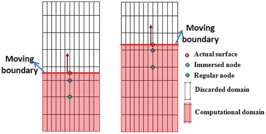
Growth of casting strand with time and implementation of Immersed boundary method at these instants.

As the upper physical boundary (i.e. meniscus) is moving upwards and the casting is growing in size, the fixed rectilinear mesh framework results into three cases for any node in the geometry at a particular time instant: the node can be inside, on the surface and outside of the billet (Figure 2). So, first, the nodes which are inside the billet (solved nodes) close to boundary of billet (immersed nodes) and on the surface of billet are identified. This identification is done at every time step to capture this position of moving boundary front before solving the temperature field for the next time level. Temperature at the inside nodes is computed by solving the finite difference equations and the temperature at nodes close to boundary front (immersed point) is interpolated from the boundary temperature and inside point’s temperature values. The interpolation function used to reconstruct the solution at these nodes is expressed as equation (3)

f (n) = {an}^{2} + bn + c

(3)

where n is the distance of the immersed grid point from the moving surface. Mittal et al.⁴⁵ presented a similar approach for solving momentum equations with a moving boundary. The immersed surface is identified and a quadratic interpolation function is used along the normal direction to specify temperature at the immersed nodes. As per Figure 2, at blue nodes (immersed points), the temperature is calculated using the interpolation of red and green nodes. The red nodes are at the actual boundary where boundary condition (T = meniscus temperature) is known to us. Green nodes are the solved nodes, which are solved directly from the finite difference form of energy equation.

Discretization methodology

Finite difference method with Forward-Time Central-Space (FTCS) scheme is used to solve this problem numerically. Explicit time integration scheme is used and a von Neumann criterion is considered for stability. Ghost cell method is used to satisfy the Neumann boundary conditions (at fixed boundaries).

Generally, time increment, Δt, is calculated on the basis of von Neumann stability criteria. The first-order upwind scheme is used for convection term. In addition to these criteria, Δt satisfied the relation (4) arising from the stability of the IBM implementation

u \times Δ t ⩽ Δ Z

(4)

Parallelization of the solver

3D transient equation is computationally intensive and needs higher computational time. So in order to reduce the computation time, a domain decomposition technique has been used, which distributes the nodes in several processors and solves each sub-domain independently. Communications among the processors are achieved using message passing interface (MPI). Thus, parallel programming has enabled us to reduce the computational time by utilizing high-performance computing resources with multi-core architecture. Figure 3 shows the current implementation up to eight processors with an almost-linear scalability.

Figure 3.

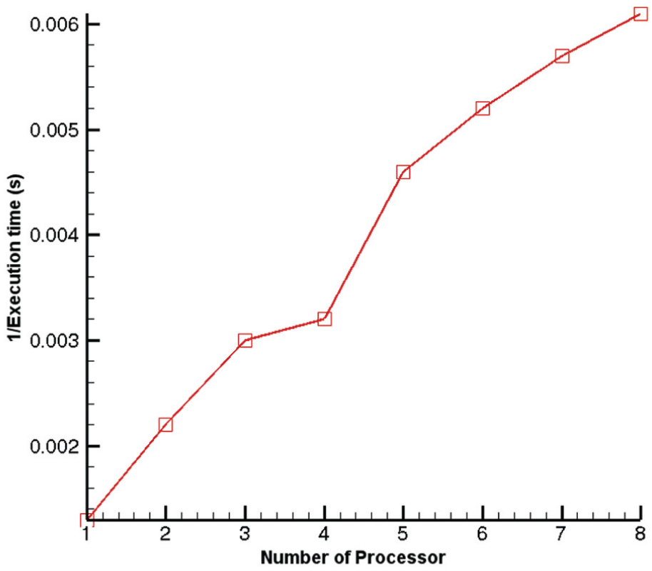
Scalability up to eight processors.

Geometry and boundary conditions

The billet is of rectangular shape and it facilitates two axes of symmetry, so only a quarter of billet has been solved with symmetric boundary conditions at the respective edges in order to reduce the simulation time. Schematic of the boundary conditions representing different cooling ambiences are depicted in Figure 4. Since the meniscus is moving, the boundary conditions at the surfaces of casting strand are also moving along with the meniscus movement to maintain the exact locations of different boundary conditions.

Figure 4.

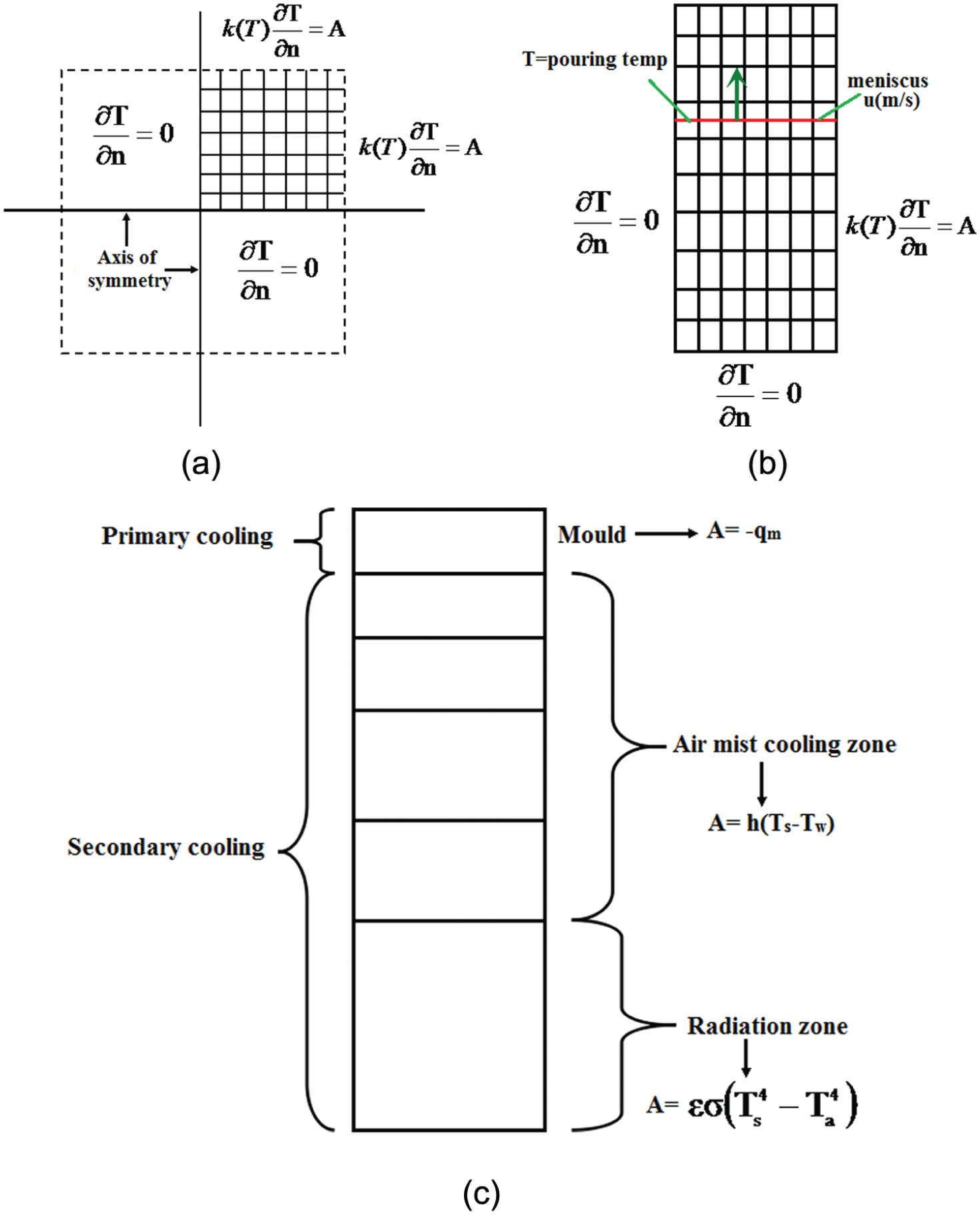
(a) Horizontal section of billet with boundary condition, (b) vertical section of billet with boundary conditions and (c) different cooling section for multi-zonal cooling ambience.

Primary zone (mould)

The heat flux extraction rate from surface of billet is expressed as equation (5)

q_{m} = h_{m} (T_{s} - T_{a})

(5)

The value of h_m could be determined by an integral heat balance on the mould. It depends upon average heat flux to the mould water and dwell time. The value of h_m could also be determined by Hill’s⁴⁶ correlation.

Secondary zone

Air/mist cooling

In this zone, a number of nozzles spray water on casting strand with different water flow rate. This is done to achieve controlled cooling. The boundary condition which replicates this phenomenon can be expressed as equation (6)

k (T) \frac{dT}{dn} = h (T_{s} - T_{w})

(6)

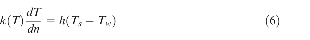
Heat transfer coefficient, h, can be expressed as equation (7) in relation to water flow rate⁴⁷

h = 116 + 10.44 W^{0.815}

(7)

Radiation zone (air cooling)

In this zone, the casting strand surface is only in contact with still air, which has negligible convection effect. The boundary can be expressed as equation (8)

k (T) \frac{dT}{dn} = q_{r}

(8)

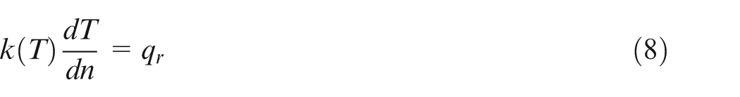
where q_r is govern by Stefan–Boltzmann’s law and expressed as equation (9)

q_{r} = ε σ (T_{s}^{4} - T_{a}^{4})

(9)

The emissivity of oxidized surface is generally taken as 0.8.¹⁰

Material data

Three different grades of steel alloys have been used for validation cases namely, 0.3 wt% C steel, 42CrMo and 5G2A steel for the set-1, set-2 and set-3, respectively. 15G2A steel alloy is used in remaining analysis (i.e. set-4 to -11). The composition and material properties of the alloys are available in the cited literature.^15,17,43,48

Results and discussion

Validation study

In order to validate this IBM model, three different benchmark cases are considered. The first two cases focus only on the mould region and the third case considers multi-zonal cooling ambiences. Attempts have been made to compare shell thickness and surface temperature predicted by this model with reported data. Shell thickness is determined as the thickness of the metal pool which has temperature less than or equal to solidus temperature.

Mould region

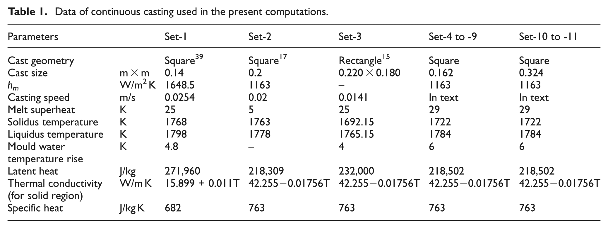
Case 1: Geometric properties and thermal boundary conditions for the first validation case are specified in set-1 (Tables 1 –3). The effective thermal conductivity for the liquid and mushy phases at electromagnetically stirred mould region has been considered as k_effective = mk with m = 2. The density is assumed to be of constant value of 7400 kg/m³ for all phases. Our predictions for solidified shell thickness are compared with radioactive tracer based measurements of Lait et al.³⁹ (Figure 5). The comparisons show good agreement only with little discrepancy at the near meniscus height. This is to be mentioned that a higher equivalent k-based model of Choudhary and Mazumdar⁴² has shown disagreement with the experimental data for a similar case. They reported good agreement only when a conjugate heat transfer simulation is performed. Our computation shows that this IBM based methodology coupled with consideration of the convective heat transfer term and a lower effective k value gives good agreement avoiding the involved computations needed for a conjugate solver.

Table 1.

Data of continuous casting used in the present computations.

Parameters		Set-1	Set-2	Set-3	Set-4 to -9	Set-10 to -11
Cast geometry		Square³⁹	Square¹⁷	Rectangle¹⁵	Square	Square
Cast size	m × m	0.14	0.2	0.220 × 0.180	0.162	0.324
h_m	W/m² K	1648.5	1163	–	1163	1163
Casting speed	m/s	0.0254	0.02	0.0141	In text	In text
Melt superheat	K	25	5	25	29	29
Solidus temperature	K	1768	1763	1692.15	1722	1722
Liquidus temperature	K	1798	1778	1765.15	1784	1784
Mould water temperature rise	K	4.8	–	4	6	6
Latent heat	J/kg	271,960	218,309	232,000	218,502	218,502
Thermal conductivity (for solid region)	W/m K	15.899 + 0.011T	42.255−0.01756T	42.255−0.01756T	42.255−0.01756T	42.255−0.01756T
Specific heat	J/kg K	682	763	763	763	763

Table 2.

Length of different section (m).

Set	Mould	WS-1	WS-2	WS-3	WS-4	RAD
1	0.5	–	–	–	–	–
2	0.6	–	–	–	–	–
3	0.8	0.57	0.74	1.49	2.70	8.4
4–9	0.5	–	–	–	–	–
10–11	0.9	2.6	2.5	4.47	12.70	9.83

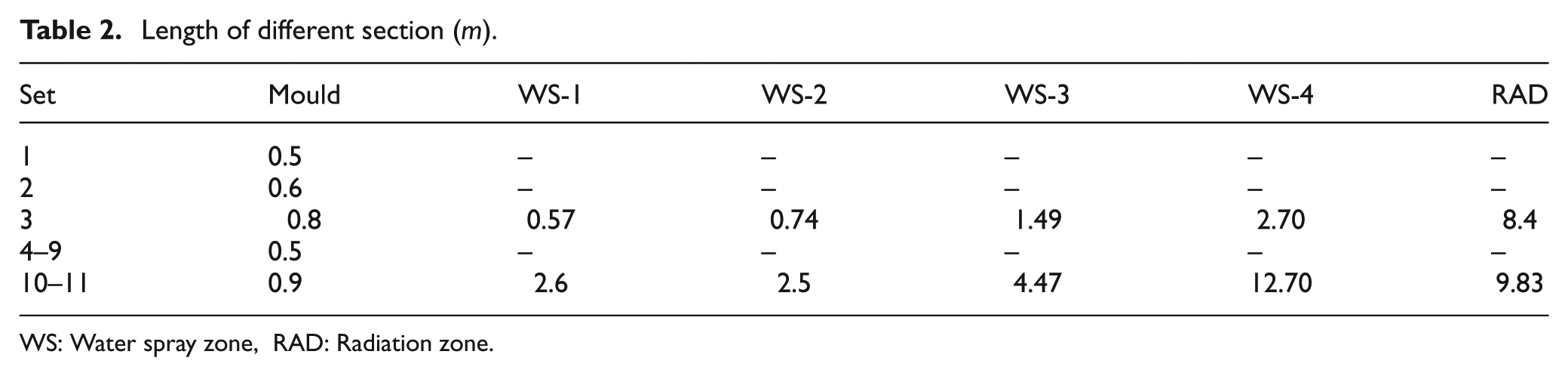
WS: Water spray zone, RAD: Radiation zone

Table 3.

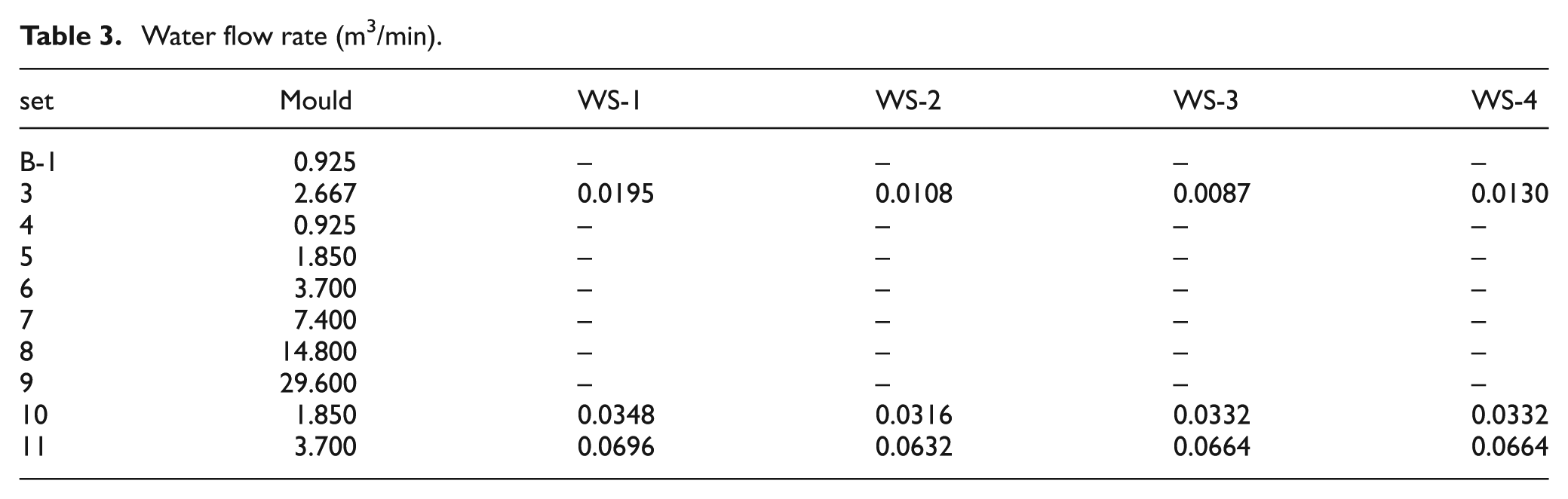
Water flow rate (m³/min)

set	Mould	WS-1	WS-2	WS-3	WS-4
B-1	0.925	–	–	–	–
3	2.667	0.0195	0.0108	0.0087	0.0130
4	0.925	–	–	–	–
5	1.850	–	–	–	–
6	3.700	–	–	–	–
7	7.400	–	–	–	–
8	14.800	–	–	–	–
9	29.600	–	–	–	–
10	1.850	0.0348	0.0316	0.0332	0.0332
11	3.700	0.0696	0.0632	0.0664	0.0664

Figure 5.

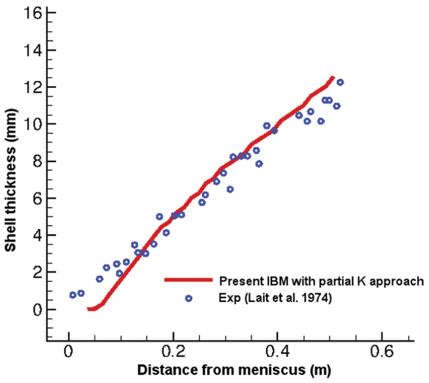
Comparison of predicted shell thickness with experimental result.

Case 2: Geometric properties and thermal boundary conditions for the first case are specified in set-2 (Tables 1 –3). Janik and Dyja⁴³ neglected the convective term due to vertical casting speed and considered a higher value of effective thermal conductivity (k_effective = 7k) through all phases to encompass the stirring effects. In this study, the similar approach is tested and in addition to that the same problem is solved using the other approach which considers the convective term due to z-movement of molten metal along with the effective k (k_effective = 2k, a lower magnitude) at the liquid and mushy phases. The densities considered for liquid, mushy and solid phases are 7000, 7200 and 7400 kg/m³, respectively.

Chipman and Fondersmith⁴⁹ showed that shell thickness is proportional to square root of solidification time for ingot casting. Savage and Pritchard⁵⁰ showed that for continuous casting, the solidification time may be estimated as, time = distance from meniscus/casting velocity. They also derived their own correlation for continuous casting. Our predictions are also compared with Chipman–Fondersmith and Savage–Pritchard correlations (Figure 6).

Figure 6.

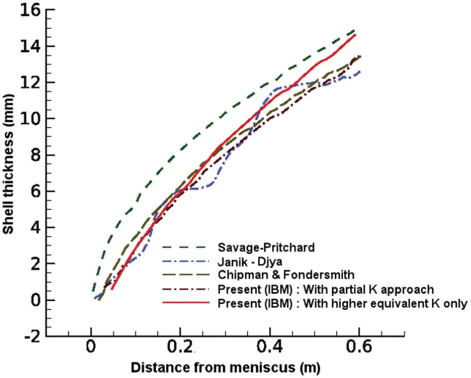
Comparison of predicted shell thickness with available results and Savage–Pritchard correlation.

Since the partial k approach (lower magnitude of equivalent k along with convective term due to movement of billet) results are best comparable with experimental as well as Chipman–Fondersmith and Savage–Pritchard correlation, this method has been used for all remaining computations presented in this article. Our prediction considering the z-directional convection agrees closely with both experimental results and established correlations, and hence, this approach can provide a very good model for continuous casting simulations.

To confirm grid-independence of the solutions, cases are run with two different grid sizes, 80 × 80 × 120 and 120 × 120 × 180. For both of the cases, shell thickness is predicted to be the same.

Multi-zonal cooling ambiences

For validation of multi-zonal ambience cooling, the case similar to the Qing et al.¹⁵ case has been simulated. The partial k approach along with convection effect is used. The set-3 (Tables 1 –3) is considered for this case. The densities considered for liquid, mushy and solid zones are 7000, 7200 and 7400 kg/m³, respectively. The effective thermal conductivity, k_effective = mk, has been considered for liquid and mushy phases, where m equals 1–2, in different cooling ambiences (or zones). The value of m is equal to 2 for mould and segment-1 and 1 for other segments. The heat extraction in mould for this case has been considered as per Savage–Pritchard⁵⁰ heat flux relation. The shell thickness with respect to metallurgical length is plotted for casting speed (u) of 0.085 m/min (Figure 7). Our prediction of shell thickness with partial k approach agrees well with Qing et al.’s result (Figure 7).

Figure 7.

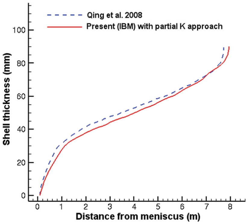
Comparison of predicted shell thickness with Qing’s results under multi-cooling ambiences.

Effect of heat extraction rate in mould region

In order to quantify the effect of the rate of heat extraction on shell growth, simulations are performed with different magnitudes of heat extraction rate. Casting velocity is kept constant at 0.0267 m/s for all the cases. The parameters are shown in set-4 to -9 (Tables 1 –3). The effective thermal conductivity, k_effective = mk, with m = 2 has been considered. 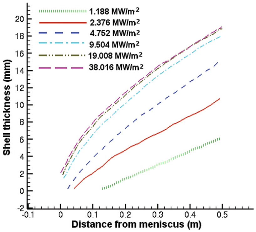The respective heat extraction rates are calculated using $dq = c_{w} \overset{\cdot}{m} Δ T$ . Results in terms of solidified shell thickness are presented in Figure 8.

Figure 8.

Predicted shell thickness for different heat extraction rates at casting speed of 0.0267 m/s.

As the shell thickness suggests a parabolic behaviour with distance from the mould (or distance travelled due to the casting speed), the shell thickness varies linearly with square root of time ( $\sqrt{t}$ ) in Figure 9. The results agree with Chipman and Fondersmith empirical relation

d = A \sqrt{t} - C

(10)

where A is considered as a constant depending on the material property and heat extraction rate; C is considered as delay constant, which is related to amount of superheat; t is time in minute and d is shell thickness in millimetre. The obtained values of A and C in Figure 9 are within the ranges reported by other authors for low carbon steel.⁵¹ It is found that at lower heat extraction rates, the Chipman and Fondersmith relation does not hold. The relation changes to

d = At - \sqrt{C}

(11)

Figure 9.

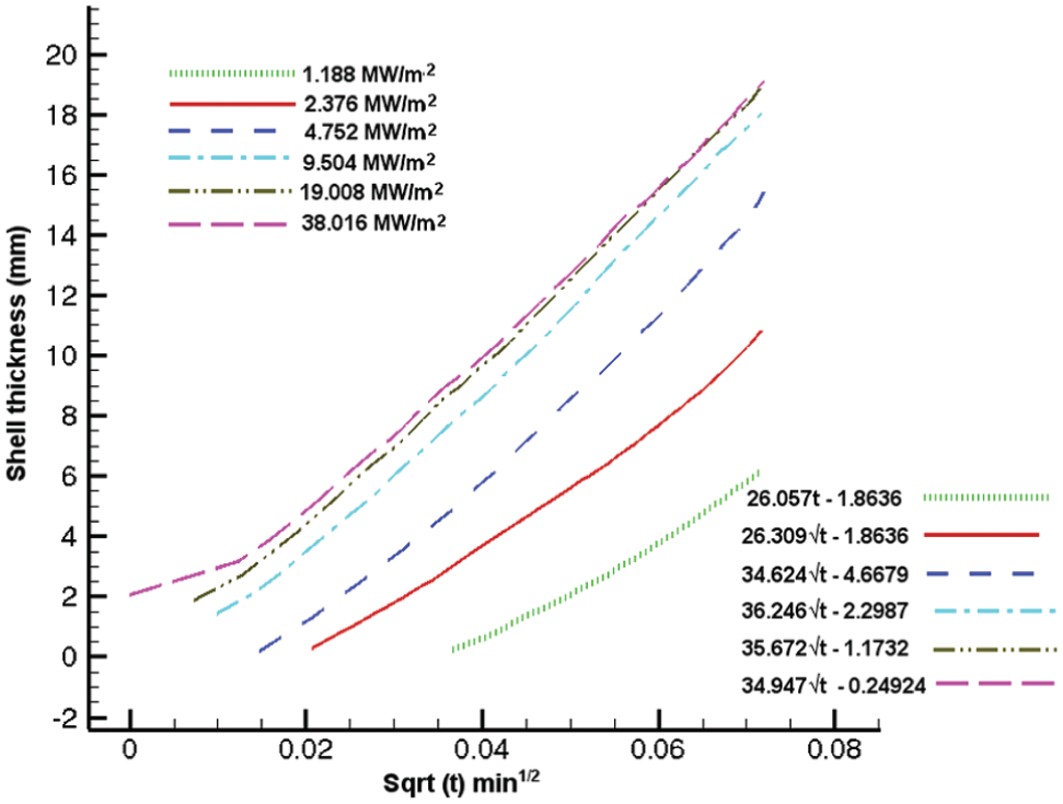
Predicted shell thickness for different heat extraction rates on square root of time scale at casting speed of 0.0267 m/s.

Due to this, the shell-thickness profile with respect to $\sqrt{t}$ does not remain linear for heat extraction of magnitude of 1.188 MW/m² (Figure 9). The corresponding solidus line, in Figure 8, is a straight line (shell thickness vs distance plot). A similar linear relationship is also reported by Hanao et al.⁵¹ for initial solidification period (t < 0.005 min), when effect of higher extraction rate is dormant. It is also observed that all higher heat extraction rates result in the Chipman and Fondersmith relation.

The effect of heat extraction rate slows down and finally ceases at higher values. In this article, heat extraction rate above 19.008 MW/m² has no further effect on shell thickness, and hence, solidified thickness profile becomes constant for higher heat extraction rates and so the value of A and C in aforesaid correlation.

Effect of casting velocity in mould region

In order to quantify the effect of the casting velocity on the growth of shell thickness inside the mould, three different velocities (0.01335, 0.0267 and 0.0534 m/s) are studied as presented in Figure 10(a) and (b), keeping heat extraction equal to 2.376 MW/m² in all cases. The other parameters are considered as shown in set-5 (Tables 1 –3).

Figure 10.

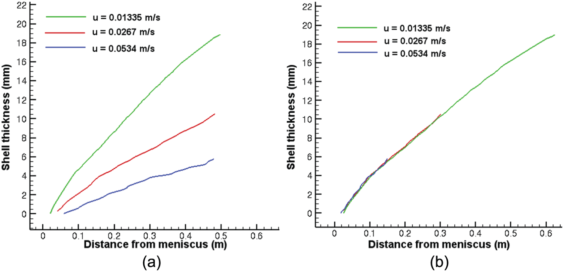
Predicted shell thickness with different casting velocities with heat extraction rate of 2.3764 MW/m² (a) with distance from meniscus and (b) with square root of time.

The results in terms of solidified shell thickness are presented with respect to distance from meniscus (Figure 10(a)) and square root of time (Figure 10(b)). Increased casting speed leads to high value of time-delay constant, and as a consequence, a low shell thickness is achieved in the mould region (this may lead to bursting). This could be observed in Figure 10(a), which shows that solidified shell starts to grow at higher distances from meniscus as the velocity increases. On the vice-versa, time delay becomes small at lower velocities. Figure 10(b) shows that the effect of velocity on temporal growth of solidified shell inside the mould region is negligible, and hence, Chipman and Fondersmith correlation holds for different casting velocities. However, the effect of velocity could be seen in terms of shell thickness with respect to distance from meniscus inside the mould. The higher speed needs more metallurgical length to achieve same amount of solidified shell thickness as compared to lower casting speed (Figure 10(a)).

Correlation for delay constant

The relation between solidified shell thickness and solidification time can be expressed as sets of modified Chipman–Fondersmith relations as shown in the legend of Figure 9:

$d = A \sqrt{t} - C$ , when heat extraction rate is of higher magnitude;

Or, $d = At - \sqrt{C}$ when heat extraction rate is of low (less than or equal to 1.188 MW/m²).

Constants A and C are functions of heat extraction rate and material properties. C denotes the time delay or minimum time needed to start solidification. This is also related with the minimum distance from the meniscus where solidified shell can start forming. For a specific material, information on C at one particular heat extraction rate (considered as reference case) can be utilized to predict values of C for other different heat extraction rates. Correlation for time-delay constant is obtained as

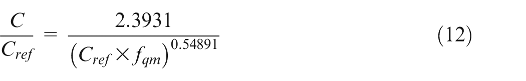
\frac{C}{C_{ref}} = \frac{2.3931}{{(C_{ref} \times f_{qm})}^{0.54891}}

(12)

where C is the delay constant, C_ref is the delay constant for the reference case and f_qm is the heat extraction rate as fraction of the reference case.

For 15G2A grade steel (low carbon steel), the value of A ranges from 26 to 36 and becomes constant for higher heat extraction rates (q_m ≥ 19 MW/m²). The correlation-fit data are shown along with the computational results in Figure 11.

Figure 11.

Shell thickness correlation and computational results.

Simulation of the full-length billet considering multi-zonal cooling ambiences

Numerical simulation on the full-length billet geometry under different cooling ambiences is performed using IB method in multiple processors (11 processors). The partial k approach (lower values of equivalent k along with convective term due to casting speed) is used. The multi-zonal cooling ambience is chosen as shown in Figure 4(c). The different values of equivalent k are used in different segments, k values are decreased away from the meniscus as the stirring/turbulence effects decrease. The effective thermal conductivity, k_effective = mk, has been considered for all temperature above solidus temperature (i.e. liquid and mushy phases), where m varies in the range of 1–3 at different cooling ambiences (or zones). The values of m are considered as m = 3 in the mould, m = 2 at segment-1 and m = 1 for other segments. The caster and casting parameters are chosen according to Tables 1 –3 (set-10 to -11).

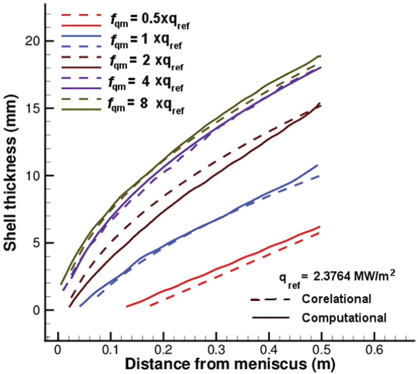
In Figure 12(a), the solidus line front and 70% solidification front are plotted against the distance from meniscus at two time different levels. The casting velocity is taken as 0.0111 m/s. It shows that once the full domain is solidified, the solidus front or 70% solidus front profile remains the same with respect of time, and the casting problem turns to a case of steady-state heat transfer.

Figure 12.

Predicted shell thickness under multi-cooling ambiences at casting speed of 0.0111 m/s (a) with distance from meniscus (at different time levels) and (b) with square root of time.

In Figure 12(b), the shell thickness with respect to square root of time is plotted. It is observed that the shell thickness is proportional to $\sqrt{t}$ for t ≤ 2.56 min (i.e. 1.7 m, which is close to mould region) and after that it deviates from linear relation. Later, when 90% shell thickness is achieved, the curve again exhibits linear variation with respect to $\sqrt{t}$ . Figure 12(a) shows that in the intermediate air-mist cooled zone, shell thickness is proportional to time, t (time is proportional to distance from meniscus). This also justifies the observation that with lower heat extraction rates, the shell thickness varies as $d \propto t$ . So in the mould and its vicinity, where extraction rate is high, $d \propto \sqrt{t}$ relation holds and away from the mould, it follows $d \propto t$ . It once again holds the $d \propto \sqrt{t}$ relation when the domain solidification reaches to more than 90%, at which heat content by liquid phase is less and moreover, the temperature of solid phase drops below 700 K at the vicinity of the boundary. At this temperature, steel has higher thermal conductivity. High values of thermal conductivity promote better heat conduction in this region and yields higher heat extraction rate (via surface convection). Hence, the solidified shell thickness follows the correlation $d \propto \sqrt{t}$ in this regime.

Figure 12(b) also shows that the 70% solidus line holds $d \propto \sqrt{t}$ for longer period of time as higher heat extraction rate will be favoured for longer metallurgical length and hence verifies our observation that there is a critical value of heat extraction rate at which the correlation switches.

Effect of casting speed on billet or multi-zonal cooling ambiences

The effects of casting velocity in multi-cooling ambiences are presented in Figure 13(a) and (b). The caster parameters are taken according to set-10 of Tables 1 –3. The three different casting speeds considered are 0.0055, 0.0111 and 0.0267 m/s, respectively. In Figure 13(a), shell thickness is plotted against the distance from meniscus, and it shows that for higher speeds, longer distance from meniscus is needed for complete solidification, which is obvious as time for solidification decreases with increase in speed. As the casting speed increases to 0.0267 m/s, the metallurgical length of the entire domain (30.2 m) does not emerge to be sufficient to achieve full solidification. However, to show the temporal effect of velocity in shell growth, shell thickness is plotted against $\sqrt{t}$ (Figure 13(b)). It has already been discussed earlier that the shell thickness is independent of speed in mould region but in multi-cooling ambiences, Figure 13(b) shows a variation in growth of shell-thickness profile for different casting speeds. This can be explained by the fact that although the shell-thickness profile is independent of velocity, time durations spent by the casting material at different cooling ambiences in the multi-zonal set-up changes at different speed levels, and hence, differences in solidification pattern are observed. So with lower casting speed, the billet stays in higher heat extraction rate (like mould region) for longer time while with higher casting speed it moves fast to lower heat extraction rate ambience (say air-mist cooling zone) where the $d \propto t$ instead of $d \propto \sqrt{t}$ .

Figure 13.

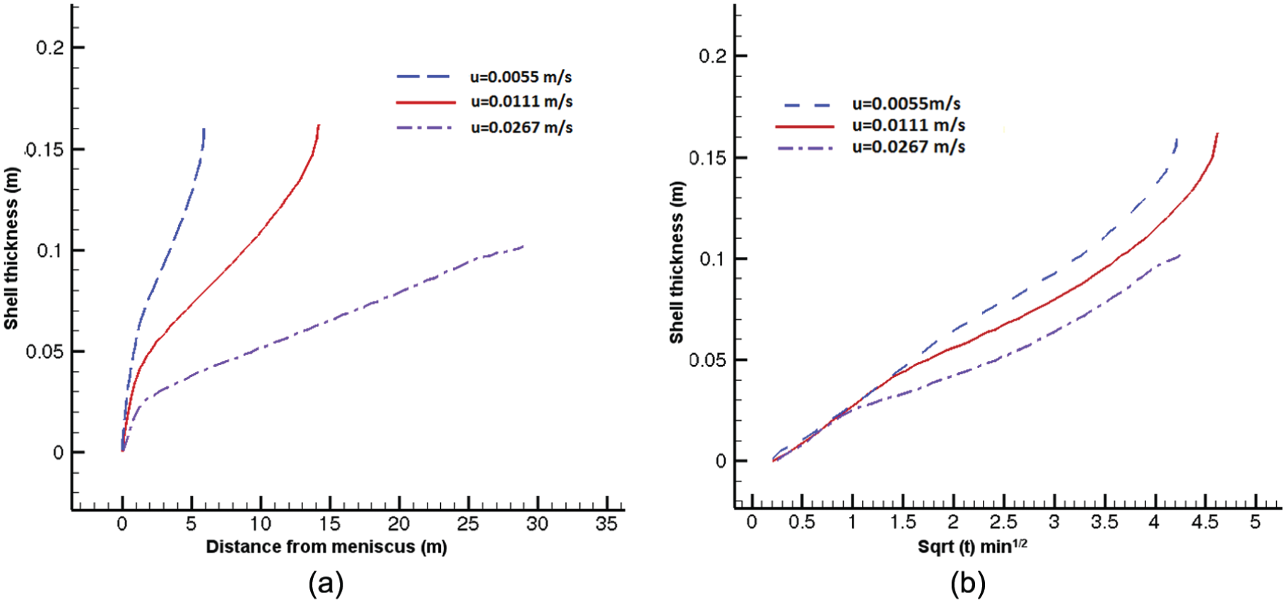
Predicted shell thickness with different casting velocities under multi-cooling ambiences (a) with distance from meniscus and (b) with square root of time.

It is also noteworthy that in Figure 13(a), a very low casting speed shows solidification of the entire casting cross section at a distance of 5 m/min from the mould. This distance increases with increase in speed and no complete solidification is observed for a higher speed of 0.0267 m/min. This observation can be attributed to the fact that with increase of speed solidification, time decreases that supersedes the enhanced convection effects and the molten alloy does not get sufficient time for solidification of the full cross section through its entire length.

So from Figure 13(b), it can be observed that the $d \propto \sqrt{t}$ up to 4.84, 2.56 and 1.21 min for case u equal to 0.0055, 0.0111 and 0.0267 m/s, respectively. All these time levels correspond to approximately 1.6 m from meniscus. Above these time levels, in both the cases, they follow $d \propto t$ and as discussed above, the $d \propto \sqrt{t}$ relation is again achieved as the shell thickness approaches to 90% domain solidification.

Effect of heat extraction rate on billet for multi-zonal cooling ambiences

The effects of heat extraction rate in multi-cooling ambiences are presented in Figure 14(a) and (b). The caster parameters are taken according to set-10 to -11 of Tables 1 –3. The casting speed is kept equal to 0.0111 m/s for both the cases. In Figure 14(a), the growth of shell thickness with respect to metallurgical length is presented while Figure 14(b) depicts shell-thickness variation with respect to square root of time. The lower and higher heat extraction rates are provided according to Table 1 and 3 (Set-10 to 11). The case with higher heat extraction rate has double heat extraction rates in every respective section as compared to the lower heat extraction rate. The effect of heat extraction is significant in terms of both metallurgical length and time scale. Increase in the heat extraction rate favours the process of shell solidification. Figure 14(b) also depicts that the slope of solidified shell remains same in both of the cases; however, a constant offset is observed. Hence, it can be inferred that a change in heat extraction rates in multi-zonal cooling ambience introduces a time delay in the solidification process.

Figure 14.

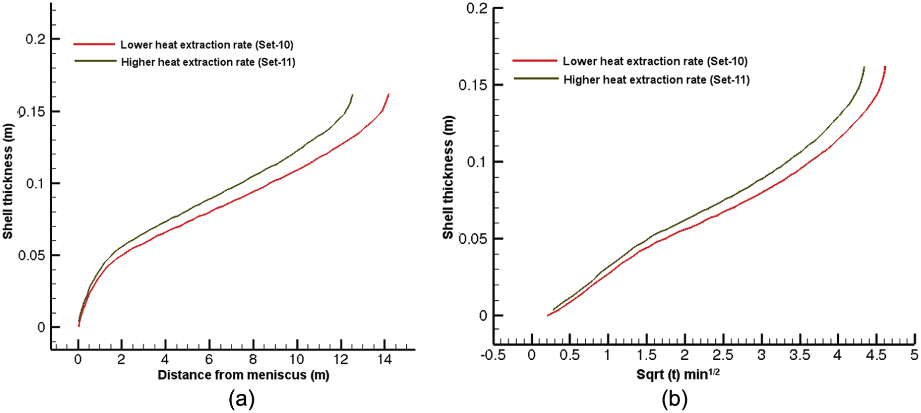
Predicted shell thickness for different with different heat extraction rates at casting speed of 0.0111 m/s (a) with distance from meniscus and (b) with square root of time.

The variation of shell thickness at different cooling ambiences can also be explained via temperature contours over an axial plane (Figure 15). The temperature contours for set-10 with casting speed of 0.0111 and 0.0267 m/s and set-11 with casting speed of 0.0111 m/s are shown for metallurgical length of 16 m. It can be seen that high temperature zone expands up to the bottom plane in set-10 with increased casting speed. The solidified region (with temperature less than solidus temperature, 1722 K) increases especially near the lower planes for set-11 with casting speed of 0.0111 m/s, which has double of heat extraction rate than set-10 with casting speed of 0.0111 m/s.

Figure 15.

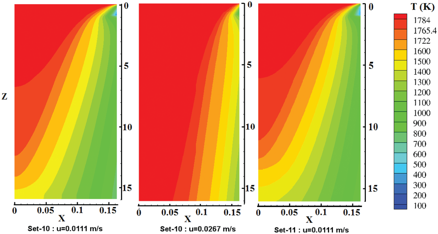
Temperature profile for different velocities and heat extraction rates.

Conclusion

This article demonstrates implementation of an efficient IBM based finite difference scheme for prediction of solidified shell thickness and temperature profile in a continuous caster. The proposed methodology shows good agreement with previously reported data as well as linear scalability over multiple processors. It is also shown that an increased effective conductivity coupled with convection term due to casting speed can better model the heat transfer augmentation due to electromagnetic stirrer. Solidification patterns are observed with respect to distance from the meniscus and time of solidification. Time-delay in solidification is found to be a function of heat extraction rate from the mould. A correlation has been proposed to determine the effect of heat extraction rate on growth of solidified shell in the mould region. It is shown that at a lower heat extraction rate, $d \propto t$ is favoured over the Chipman–Fondersmith correlation.

Different cooling ambiences (as used in an industrial continuous caster) have been tested and their effect in the shell thickness has been studied. It is observed that higher heat extraction rate and lower casting speed favour better solidification. The 3D heat transfer and solidification patterns are visualized to explore thermal physics of continuous casting. Graphically, the metallurgical length could be determined with change in casting speed if the data for growth of shell thickness for one case is known.

The present results and the obtained correlations can be utilized to obtain a pool of information for different cooling parameters and casting speeds, which could be helpful while designing the caster for better productivity and to avoid bursting or breakout. The proposed IB model also offers potential for simulation of complex casting configuration with moving boundaries. Furthermore, this method can be used to study the heat transport phenomena in other manufacturing processes which involve complex geometries with fixed or moving surfaces (like investment casting, friction stud welding).

Footnotes

Appendix 1 Declaration of conflicting interests

The authors declared no potential conflicts of interest with respect to the research, authorship, and/or publication of this article.

Funding

The author(s) disclosed receipt of the following financial support for the research, authorship, and/or publication of this article: This work has been financially supported by BRNS grant 2012/34/68/BRNS/2972. Computations are performed using HPC infrastructures at IIT Patna.

References

Seah

KHW

Hemanth

Sharma

. Effect of high-rate heat transfer during casting on the strength, hardness and wear behaviour of aluminium-quartz particulate metal matrix composites. Proc IMechE, Part B: J Engineering Manufacture 2003; 217(5): 651–659.

Pagratis

Karagiannis

Vosniakos

. A holistic approach to the exploitation of simulation in solid investment casting. Proc IMechE, Part B: J Engineering Manufacture 2007; 221(6): 967–979.

Ei-Kaddah

Natrajan

. Electromagnetic stirring of steel: effect of stirrer design on mixing in horizontal electromagnetic stirring of steel slabs. In: Second international conference on CFD in the minerals and process industries, CSIRO, Melbourne, VIC, Australia, 6–8 December 1999. Available at: http://www.cfd.com.au/cfd_conf99/Conf99_Papers/085EL.PDF

Moffatt

. Electromagnetic stirring. Phys Fluids A: Fluid 1991; 3: 1336–1343.

Spitzer

Dubke

Schwerdtfeger

. Rotational electromagnetic stirring in continuous casting of round strands. Metall Trans B 1986; 17: 119–131.

Reddy

TVS

Dwivedi

Jain

. Effect of stir-casting on the microstructure and adhesive wear characteristics of cast Al–Si–Cu alloy. Proc IMechE, Part B: J Engineering Manufacture 2009; 223(1): 83–87.

Moinet

. The free meniscus problem in the continuous casting of steel: a computational model of cast surface formation. ProQuest Dissertations and Thesis, Carnegie Mellon University, Pittsburgh, PA, 2012, p.335.

Jin

Bae

Kang

. Development of rheology vacuum low-pressure die casting with electromagnetic stirrer and vacuum system. Proc IMechE, Part B: J Engineering Manufacture 2014; 228: 1599–1610.

Mizikar

. Mathematical heat transfer model for solidification of continuous casting of steel slabs. Trans Metall Soc Am Inst Min Metall Petrol Eng 1967; 239: 1747–1753.

10.

Brimacombe

. Design of continuous casting machines based on a heat-flow analysis: state-of-the-art review. Can Metall Quart 1976; 15: 163–175.

11.

Thomas

. Transient thermal model of the continuous single-wheel thin-strip casting process. Metall Mater Trans B 1996; 27: 509–525.

12.

Lally

Biegler

Henein

. Finite difference heat-transfer modelling for continuous casting. Metall Trans B 1990; 21: 761–770.

13.

Meng

Thomas

. Heat transfer and solidification model of continuous slab casting: CON1D. Metall Mater Trans B 2003; 34: 685–705.

14.

Alizedeh

Edris

Shafyei

. Mathematical modeling of heat transfer for steel continuous casting process. Int J ISSI 2006; 3(2): 7–16.

15.

Qing

Liangzhou

Liqiang

. Mathematical model of heat transfer for bloom continuous casting. J Univ Sci Technol B 2008; 15: 17–23.

16.

Tieu

Kim

. Simulation of the continuous casting process by a mathematical model. Int J Mech Sci 1997; 39: 185–192.

17.

Janik

Dyja

. Modelling of three-dimensional temperature field inside the mould during continuous casting of steel. J Mater Process Technol 2004; 157–158: 177–182.

18.

Malamataris

Papanastasiou

. Analysis of high-speed continuous casting with inverse finite elements. Int J Numer Meth Fl 1991; 13: 1207–1223.

19.

Boehmer

Fett

Funk

. Analysis of high-temperature behavior of solidified material within a continuous casting machine. Comput Struct 1993; 47: 683–698.

20.

Majchrzak

. Numerical simulation of continuous casting solidification by boundary element method. Eng Anal Bound Elem 1993; 11: 95–99.

21.

Siegel

. Analysis of solidification interface shape during continuous casting of a slab. Int J Heat Mass Tran 1978; 21(11): 1421–1430.

22.

Das

Sarkar

. Computational modelling of thermal transport phenomena in continuous casting process based on non-orthogonal control volume approach. Commun Numer Meth Eng 1996; 12: 657–671.

23.

Khosravifard

Hematiyan

Marin

. Determination of optimum cooling conditions for continuous casting by a meshless method. Proc IMechE, Part C: J Mechanical Engineering Science 2012; 22: 1022–1035.

24.

Anderson

Gethin

Lewis

. Experimental investigation and finite element modelling in gravity die casting. Proc IMechE, Part B: J Engineering Manufacture 1997; 211(2): 93–107.

25.

Song

Kovacevic

. Numerical and experimental study of the heat transfer process in friction stir welding. Proc IMechE, Part B: J Engineering Manufacture 2003; 217(1): 73–85.

26.

Soe

. Improving dimensional accuracy in the production of a CastForm™ polystyrene pattern for investment casting. Proc IMechE, Part B: J Engineering Manufacture 224(11): 1663–1670.

27.

Peskin

. Flow patterns around heart valves, A numerical method. J Comput Phys 1972; 10: 252–271.

28.

Tseng

Ferziger

. A ghost-cell immersed boundary method for flow in complex geometry. J Comput Phys 2003; 192: 593–623.

29.

Kang

. An improved immersed boundary method for computation of turbulent flows with heat transfer. Doctoral Dissertation, Stanford University, Stanford, CA, 2008.

30.

Bringley

. Analysis of the immersed boundary method for stokes flow. Doctoral Dissertation. New York University, New York, 2008.

31.

Verzicco

Mohd-Yusof

Orlandi

. Large eddy simulation in complex geometry configurations using boundary body forces. AIAA J 2000; 38: 427–433.

32.

Haworth

Jansen

. Large-eddy simulation on unstructured deforming meshes: towards reciprocating IC engines. Comput Fluids 2000; 29: 493–534.

33.

Tyagi

Acharya

. Large eddy simulation of turbulent flows in complex and moving rigid geometries using the immersed boundary method. Int J Numer Meth Fl 2005; 48: 691–722.

34.

Mittal

Iaccarino

. Immersed boundary methods. Annu Rev Fluid Mech 2005; 37: 239–261.

35.

Gilmanv

Acharya

. A computational strategy for simulating heat transfer and flow past deformable objects. Int J Heat Mass Tran 2008; 51: 4415–4426.

36.

Fadlun

Verzicco

Orlandi

. Combined immersed-boundary finite-difference methods for three-dimensional complex flow simulations. J Comput Phys 2000; 161: 30–60.

37.

Yildrim

Sun Lin

Mathur

. A parallel implementation of fluid-solid interaction solver using an immersed boundary method. Comput Fluids 2013; 86: 251–274.

38.

Anupindi

Delorme

Shetty

. A novel multiblock immersed boundary method for large eddy simulation of complex arterial hemodynamics. J Comput Phys 2013; 254: 200–218.

39.

Lait

Brimacombe

Weinberg

. Mathematical modelling of heat flow in the continuous casting of steel. Ironmak Steelmak 1974; 1: 90–97.

40.

Louhenkilpi

Laitinen

Nieminen

. Real-time simulation of heat transfer in continuous casting. Metall Trans B 1993; 24: 685–693.

41.

Saraswat

Maijer

Lee

. The influence of mould flux on the heat transfer in continuous casting. In: ICS proceedings, Charlotte, NC, 9–12 May 2005. Warrendale: AIST.

42.

Choudhary

Mazumdar

. Mathematical modelling of transport phenomena continuous casting of steel. ISIJ Int 1994; 34: 584–592.

43.

Janik

Dyja

. Modelling of three-dimensional thermal field in mould during continuous casting of steel. In: Proceedings of 11th international scientific conference achievements in mechanical and materials engineering, Gliwice, 15–18 December 2002. Poland: AMME.

44.

Comini

Guidice

Lewis

. Finite element solution of non-linear heat conduction problems with special reference to phase change. Int J Numer Meth Eng 1974; 8: 613–624.

45.

Mittal

Dong

Bozkurttas

. A versatile sharp interface immersed boundary method for incompressible flows with complex boundaries. J Comput Phys 2008; 227: 4825–4852.

46.

Hill

AWD

. Simplified theoretical treatment for transfer of heat in continuous-casting machine moulds. J Iron Steel I 1965; 203: 18.

47.

Cai

. Theory and technology of continuous casting of steel. Beijing, China: The Metallurgical Industry Press, 1999, p.277.

48.

Irving

. Continuous casting of steel. London: The Institute of Materials, 1993.

49.

Chipman

Fondersmith

. Rate of solidification of rimming ingots. Trans AIME 1937; 125: 370–377.

50.

Savage

Pritchard

. The problem of rupture of the billet in the continuous casting of steel. J Iron Steel I 1954; 178: 269–277.

51.

Hanao

Kawamoto

Yamanaka

. Growth of solidified shell just below the meniscus in continuous casting mold. ISIJ Int 2008; 49: 365–374.

Numerical simulation of continuous casting of steel alloy for different cooling ambiences and casting speeds using immersed boundary method