Sage Journals: Discover world-class research

Abstract

For years, there have been tremendous endeavors to reduce makespan in an attempt to decrease the production expenses. This investigation aims to develop a scenario-based robust optimization approach for a real-world flow shop with any number of batch processing machines. The study assumes there are some uncertainties associated with processing times as well as size of jobs. Each machine can process multiple jobs simultaneously as long as the machines’ capacities are not violated. In order to verify this developed model and to evaluate the performance of the proposed robust model, a number of test problems are prepared and a commercial optimization solver is adopted to solve these test problems. For the purpose of validating the results, the robust model and mean-value model are carried out by simulation, which confirmed the proposed model.

Keywords

Robust optimization batch processing machine scheduling uncertainty flow shop

Introduction

In batch processing machine (BPM), several jobs can be processed at the same time in such a way that all the jobs in a batch start and complete their processing, simultaneously. Semiconductor burn-in operations; environmental stress-screening (ESS) chambers; chemical, food, and mineral processing; pharmaceutical and construction materials industries; and so on are examples of BPM.¹ This research is motivated by a BPM real-world application in a printed circuit board (PCB)² assembly line originally presented by Damodaran and Srihari.³Figure 1 shows a BPM where assemblies from in circuit testing (ICT) arrive at the ESS chambers; they should be gathered in batches and the batches should be scheduled on the chambers. As it can be observed in Figure 1, the environment of chambers is a flow shop environment with m ESS chambers, and in our problem, ESS chambers are BPMs and assemblies are jobs.

Figure 1.

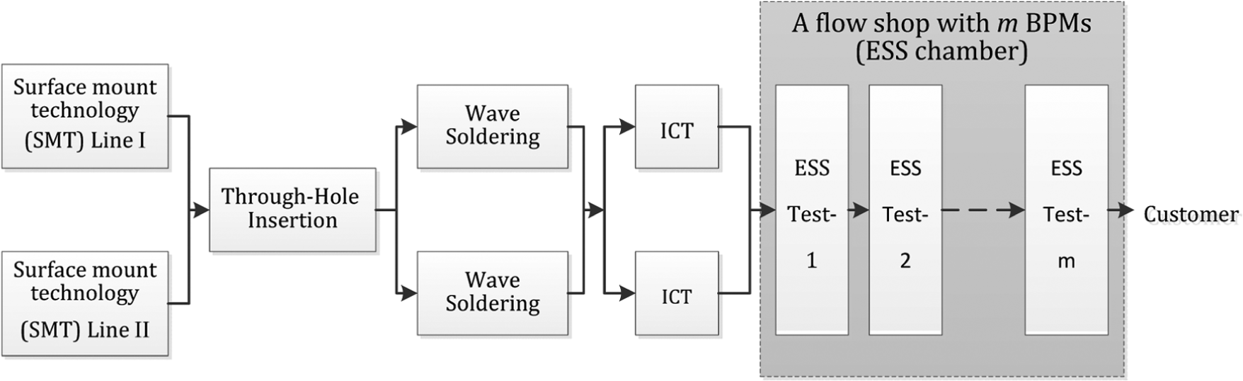
A typical printed circuit board assembly line (Source: adapted from Manjeshwar et al., 2009).

In the literature, the BPM scheduling has been divided into two main groups. The first category consists of a single BPM scheduling.^4–15 In the same order, some articles considered parallel BPM scheduling environment.^13,16–22 Moreover, for two BPM flow-shop scheduling, refer to Damodaran and Srihari.³

Shukla et al.²³ investigated sequencing a set of batches in multi-stage supply chain, and for fulfilling this purpose, a mathematical programming model is presented. Three objective functions, namely, minimization of lead time, blocking time, and due date violation were taken into account. Due to the combinatorial nature of the problem, a metaheuristic, artificial immune system (AIS) is implemented.

Evidently, the majority of studies on this topic addressed the single and two BPMs, while the number of BPMs within an assembly line could vary from 1 to m machines.

In addition, the typical assumption of a scheduling problem in the literature is known with deterministic input data, while there are many environmental noises in practical scheduling applications. These noises and uncertainties may adversely affect the inputs and substantially undermine the efficiency of outputs.²⁴ Fortunately, in recent researches, uncertainty of parameters has attracted a considerable attention.^25,26 As a result, it is necessary to develop an approach to address the problem of BPM scheduling in uncertain environment, where it can generate both efficient and reliable scheduling for real-world BPM problem.

To encounter the uncertain processing time, in some researches, specific random distribution is devised. By means of stochastic optimization approach, they solved the problem by defining their expected values in the objective functions,^27–29 and Rossi³⁰ suggested a proactive scheduling approach, which deals with fluctuations of uncertain parameters in future. Therefore, a robust optimization approach is used to formulate the uncertainty of processing times by considering all possible future scenarios.

Jensen³¹ developed robust schedules in a job shop environment by considering machine’s breakdowns to minimize makespan as a performance measure. His concept assumes that the robust solution can be found in wider regions of distribution (objective) function and vulnerable solutions are usually located on the peaks’ distribution functions. Bouyahia et al.³² assumed that the number of arrival jobs to be processed on parallel machines is a random variable. They presented a method for considering the robustness of a pre-scheduling simultaneously. Their approach minimizes the flow time as an objective function.

Al-Fawzan and Haouari³³ considered a project scheduling with uncertain task durations and constraint in resources. They presented a multi-criteria robust scheduling model, which minimizes makespan. They also defined robustness measure of scheduling as the sum of free slacks of activities. Chtourou and Haouari³⁴ proposed a two-stage algorithm to generate robust resource-constrained project scheduling subjected to unpredictable increase in processing times. Raja et al.³⁵ considered a fuzzy approach for uniform parallel machine earliness—tardiness with uncertain processing times. Another example of utilizing the fuzzy logic in scheduling problems is Wan and Chou²² that worked on fuzzy scheduling feedback algorithms.

Recently, Rahmani and Heydari²⁵ considered robust and stable flow shop scheduling with unexpected arrivals of new jobs and uncertain processing times. They used a scenario-based robust stochastic optimization approach. Nonetheless, the practical issue of robust model for non-deterministic or uncertain problem in BPM scheduling has not been tackled so far.

As it is obvious from the literature, a majority of studies have been focused on single or two BPMs while in the real world, the assembly line could consist of several BPMs. Moreover, there have been lots of ignored uncertainties which may hamper the efficiency of the outcomes. To obviate this gap, in this article, a scenario-based robust optimization model is presented for real-world flow shop problems with any number of BPMs in which the processing time and size of job are uncertain. In order to verify the developed model and to evaluate the performance of proposed robust model, a number of test problems are generated and a commercial optimization solver is adopted to solve these test problems. Then, the results of implementation robust model and mean-value model (MVM) are carried out by simulation. The results show that recommended model can reach better performance throughout realizations.

The remaining of the article is organized as follows. In section “Scenario-based robust optimization,” the robust optimization (RO) approach is explained in detail. In section “Problem description,” our BPM scheduling problem is described, and the related assumptions, parameters, and variables are introduced; also mathematical models are suggested for the problem. Then, the robust counterpart of the proposed model is presented and its related assumptions, parameters, and variables are introduced. In section “Experimental results,” computational results are reported and the robust model performance is evaluated. Finally, section “Conclusion” covers conclusion and recommendations for future researches.

Scenario-based robust optimization

The optimization problems have two different constraints:³⁶ (1) a structural constraint that is fixed and free of any noises in its input data and (2) a control constraint that is affected by noisy inputs. In addition, two sets of variables are defined: $x \in R^{n 1}$ indicates the vector of design decision variables and $y \in R^{n 2}$ denotes the vector of control decision variables. The first group of decision variables, which are named design decision variables, could be adjusted once but the control decision variables, which are the second group of decision variables, are subjected to the adjustment while the uncertain parameters are changed. The optimal value of control variables depends both on the realization of uncertain parameters and the optimal value of the design variables. The optimization model proposed by Mulvey et al.³⁶ has the following structure

Min : c^{T} x + d^{T} y

(1)

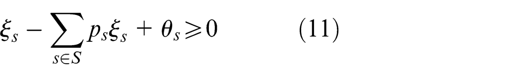
Subject to (s.t.)

Ax = b

(2)

Bx + Cy = e

(3)

x, y ⩾ 0

(4)

Equation (2) denotes the structural constraints, the coefficients of which are fixed and free of noise. Constraint (3) depicts the control constraints and their coefficients are subject to an uncertainty. For the formulation of model into robust optimization model, a set of scenarios $Ω = {1, 2, 3, \dots, S}$ is introduced. Under each scenario $s \in Ω$ , the set ${d_{s}, B_{s}, C_{s}, e_{s}}$ contains the coefficients’ values of control constraints in realization, and the probability of the scenario $p_{s} (\sum_{s = 1}^{S} p_{s} = 1)$ is associated. The optimal solution of the above mathematical programming (1)–(4) will be “robust regard to optimality” if it remains in a close proximity to its optimal value for any realization of the scenario $s \in Ω$ . This solution criterion is called “solution robustness.” Also, the solution could be “robust regard to feasibility” if it remains almost feasible for any realization of $s \in Ω$ and this solution criterion is called “model robustness.” ${y_{1}, y_{2}, \dots, y_{3}}$ is the set of control variables for each scenario $s \in Ω$ , and ${δ_{1}, δ_{2}, \dots, δ_{s}}$ is the set of error vectors. These sets are defined for the purpose of measuring the allowed infeasibility in the control constraints under each scenario $s \in Ω$ . Consider now the following formulation of the robust model

Min σ (x, y_{1}, y_{2}, \dots, y_{s}) + ω ρ (δ_{1}, δ_{2}, \dots, δ_{s})

(5)

s.t.

Ax = b

(6)

B_{s} x + C_{s} y_{s} + δ_{s} = e_{s} for all s \in Ω

(7)

x ⩾ 0, y_{s} ⩾ 0 for all s \in Ω

(8)

In the occurrence of each scenario, the objective function (1) $ξ = c^{T} x + d^{T} y$ becomes a random variable taking the value $ξ_{s} = c^{T} x + d_{s}^{T} y_{s}$ , with probability $p_{s}$ . The expected value is used for the first term in objective function (5), that is, $σ (x, y_{1}, y_{2}, \dots, y_{s}) = \sum_{s \in Ω} p_{s} ξ_{s}$ . The second term in objective function (5) called the feasibility penalty function is used in order to penalize violations of the control constraints under some of the scenarios. The goal programming weight ω is used to trade-off between solution and model robustness. A constant (λ) times the variance, that is, $λ \sum_{s \in S} p_{s} (ξ_{s} - \sum_{s' \in S} p_{s'} ξ_{s'})^{2}$ can be pulsed to $σ (x, y_{1}, y_{2}, \dots, y_{s})$ which is used for variance of cost. Yu and Li³⁷ realized that minimizing variance cost of robust optimization model takes a great deal of computation because of its quadratic forms in formulation. They suggested a new formulation for $σ (x, y_{1}, y_{2}, \dots, y_{s})$ versus previous variance cost, which has the following form

σ (x, y_{1}, y_{2}, \dots, y_{s}) = \sum_{s \in Ω} p_{s} ξ_{s} + λ \sum_{s \in S} p_{s} | ξ_{s} - \sum_{s' \in S} p_{s'} ξ_{s'} |

(9)

While objective (9) is a non-linear function, it could be optimized simply by transforming the problem into a linear programming model which has a linear objective function with linear constraints by presenting two non-negative deviational factors.

In this research, the RO used in the BPM scheduling problem is as follows

\begin{matrix} Min Z = \sum_{s \in Ω} p_{s} ξ_{s} + λ \sum_{s \in S} p_{s} [(ξ_{s} - \sum_{s' \in S} p_{s'} ξ) + 2 θ_{s}] \\ + ω \sum_{s \in S} p_{s} δ_{s} \end{matrix}

(10)

s.t.

ξ_{s} - \sum_{s \in S} p_{s} ξ_{s} + θ_{s} ⩾ 0

(11)

Ax = b

(12)

B_{s} x + C_{s} y_{s} + δ_{s} = e_{s} for all s \in Ω

(13)

x ⩾ 0, y_{s} ⩾ 0, θ_{s} ⩾ 0 for all s \in Ω

(14)

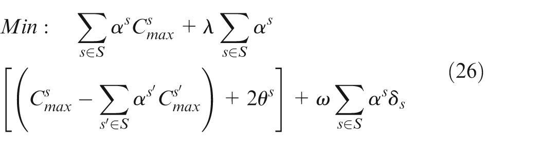
Problem description

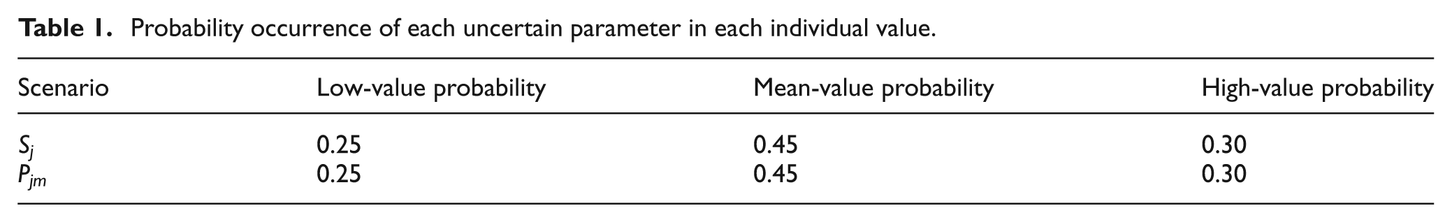
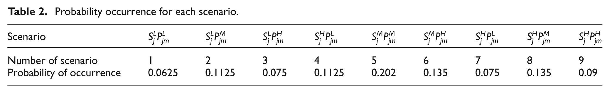
In this problem, jobs arrive to BPMs according to the accomplished estimated size of jobs, and with respect to the capacity of each machine, those jobs grouped together in a batch are determined. This batching should be done in a way that the capacity of each machine is not violated and simultaneously the makespan is minimized. Assume that the size of jobs ( $S_{j}$ ) and processing time ( $P_{jm}$ ) of jobs on each machine are subjected to uncertainty. This uncertainty in value of these parameters can be caused by many reasons, for example, tolerance in production can cause uncertainty in size of jobs, and environmental noises can change the value of process time of each job.

Each uncertain parameter has three scenarios which contain low, mean, and high values. In the plain language, the value of these parameters can be greater, equal, or less than the estimated value. It should be noted that the size of jobs and process time are two independent parameters. Therefore, each subsequent scenario of these parameters can occur independently so the total number of scenarios is equal to nine. The formation of these scenarios is shown in Figure 2, and it means if the size of jobs is less, equal, or higher than the estimated value, process time could be less, equal, or higher than its estimated value. The letters L, M, and H as superscripts mention to low, mean, and high values of the uncertain parameters, respectively.

Figure 2.

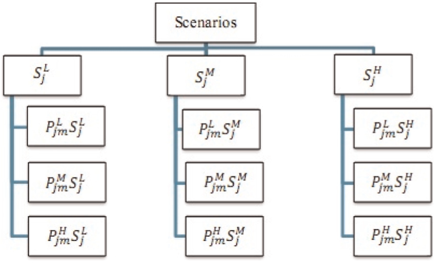
The enumeration of scenarios in the problem.

The arrival jobs to the BPMs have to pass the following steps:

Step 1: in the first step, the jobs that are decided to be in a same batch and the sequence of batches on BPMs should be determined at the beginning of the production horizon.

Step 2: according to the determined sequence of batches in the previous step, processing on batches on first BPM will start. Now it is identified that the size of some of the batches is more than the related machines’ capacity. This incident happens because of the aforementioned uncertainty in job sizes. If the size of a batch exceeds the capacity of the machine, it will be set aside. Moreover, in this step, it will be cleared which scenario for job sizes is ongoing.

Step 3: processing on batches that do not violate the capacity of the machines, but process time on each job and each machine is subjected to uncertainty and it is not clear which scenario for process time is ongoing.

Step 4: after finishing Step 3, the real job sizes are identified; therefore, batches that are set aside in Step 2 should be opened, and the parts should be extracted and batched again. In this step, with respect to the mentioned awareness about job sizes, new batching of jobs will be accomplished, but un-batching and batching process is time-consuming and it will increase the makespan.

Step 5: processing on the batches that are batched in Step 4 would be done and makespan is calculated in this step. In Figure 3, Steps 1–5 are shown in a flowchart.

Figure 3.

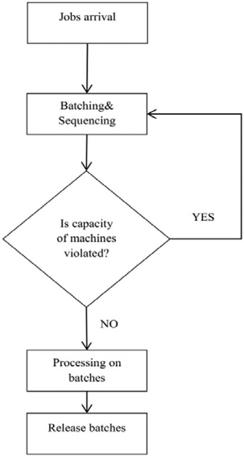
The problem flowchart.

Notations of the model

Sets

B batches which $b \in B$

J jobs which $j \in J$

K positions in sequence which $k \in K$

M machines which $m \in M$

S index for scenarios $s \in S$

Parameters

Cap capacity of machine

$P_{jm}^{s}$ processing time of job j on machine m under scenario s

$S_{j}^{s}$ size of job j under scenario $s \in S$

$α^{s}$ probability of each scenario $s \in S$

Decision variables

$X_{jb}$ binary variable indicates the assignment of job j to batch b

Dependent variables

$C_{km}^{s}$ completion time of the kth batch on machine m under scenario s

$C_{\max}^{s}$ completion time of the last batch on the last machine (makespan) scenario s

$Q_{jm}^{s}$ processing time of batch b on machine m under scenario s

MVM for BPM’s scheduling problem

Based on the suggested model by Damodaran and Srihari,³ the flow shop with m machines and the mathematical programming model according to the above-mentioned parameters and variables are as follows which is entitled MVM

Min Cmax

(15)

s.t.

\sum_{b ε B} X_{jb} = 1 \forall j \in J

(16)

\sum_{j \in J} S_{j}^{M} \cdot X_{jb} ⩽ Cap \forall b \in B

(17)

P_{jm}^{M} \cdot X_{jb} ⩽ Q_{bm} \forall b \in B, m \in M, j \in J

(18)

C_{1 m} = \sum_{m \in M} Q_{1 m}, m \in M

(19)

C_{k 1} = \sum_{k \in K} Q_{k 1}, k \in K \ {1}, s \in S

(20)

C_{km} ⩾ Q_{km} + C_{k - 1, m}, m \in M \ {1}, k \in K \ {1}, s \in S

(21)

C_{km} ⩾ Q_{km} + C_{k, m - 1}, m \in M \ {1}, k \in K \ {1}, s \in S

(22)

C_{\max} ⩾ C_{km}, k \in K, s \in S

(23)

X_{jb} binary

(24)

C_{\max}, C_{km}, Q_{bm} ⩾ 0

(25)

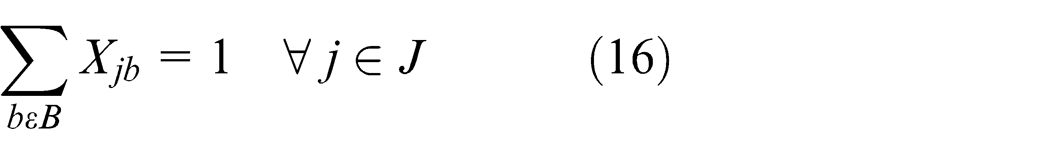
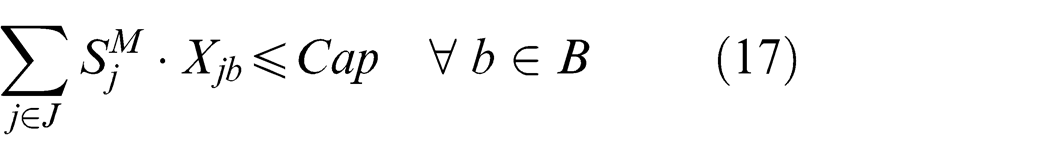
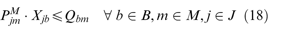
In the above-mentioned model, the mean value of uncertain parameters is considered for modeling the flow shop scheduling problem with m machines. The objective function (15) minimizes the makespan and equation (16) assures to assign each job just to one batch. Meanwhile, equation (17) guarantees no violation in machines’ capacity. Constraint (18) puts a rule which actual batch processing time to become equal to the longest processing time of all the jobs in the batch.

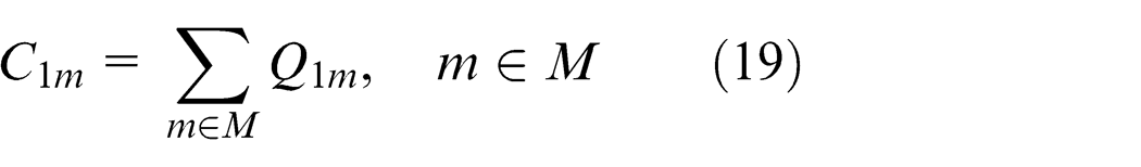
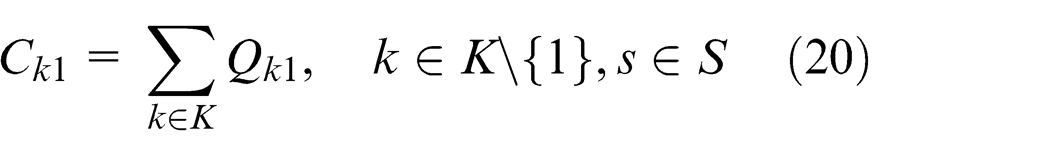
The completion time of the first batch in sequence on machine m is computed in equation (19), and the completion time of the kth batch in sequence on the first machine is calculated in limitation (20). The completion time of the kth batch in sequence on machine m is calculated in constraints (21) and (22), and then equation (23) computes the makespan. Equation (24) enforces the binary constraint on X_jb decision variable, and finally, equation (25) puts a rule on the non-negativity requirement on C_max, C_km, and Q_bm, dependent variables.

Robust model for BPM’s scheduling

As mentioned before, parameters $S_{j}$ and $P_{jm}$ are subjected to uncertainty which should be considered in modeling of the problem. The mentioned scenario-based robust optimization approach is adopted in this BPM’s scheduling problem. According to problem description, $X_{jb}$ is the only design variable, while other variables are control variables, so the robust model for BPM’s scheduling problem based on Mulvey et al.³⁶ and Yu and Li³⁷ is as follows

\begin{matrix} Min : \sum_{s \in S} α^{s} C_{\max}^{s} + λ \sum_{s \in S} α^{s} \\ [(C_{\max}^{s} - \sum_{s' \in S} α^{s'} C_{\max}^{s'}) + 2 θ^{s}] + ω \sum_{s \in S} α^{s} δ_{s} \end{matrix}

(26)

s.t.

(C_{\max}^{s} - \sum_{s' \in S} α^{s} C_{\max}^{s}) + θ^{s} ⩾ 0 s \in S

(27)

\sum_{b \in B} X_{jb} = 1 \forall j \in J

(28)

\sum_{j \in J} S_{j}^{s} \cdot X_{jb} ⩽ Cap + δ_{s} \forall b \in B, s \in S

(29)

P_{jm}^{s} \cdot X_{jb} ⩽ Q_{bm}^{s} \forall b \in B, m \in M, j \in J, s \in S

(30)

C_{1 m}^{s} = \sum_{j}^{m} Q_{1 j}^{s}, m \in M, s \in S

(31)

C_{k 1}^{s} = \sum_{j}^{k} Q_{j 1}^{s} k \in K \ {1}, s \in S

(32)

C_{km}^{s} ⩾ Q_{km}^{s} + C_{k - 1, m}^{s} m \in M \ {1}, k \in K \ {1}, s \in S

(33)

C_{km}^{s} ⩾ Q_{km}^{s} + C_{k, m - 1}^{s} m \in M \ {1}, k \in K \ {1}, s \in S

(34)

C_{\max}^{s} ⩾ C_{km}^{s} k \in K, s \in S

(35)

X_{jb} binary, C_{\max}^{s}, C_{km}^{s}, Q_{bm}^{s} ⩾ 0

(36)

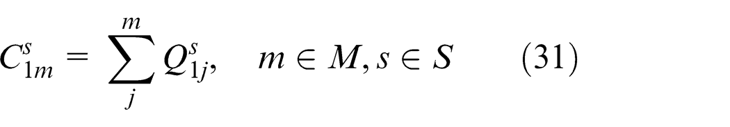
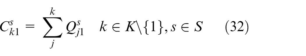
The objective function (26) minimizes the expected value and variance of scenarios’ makespan and infeasibility of constraint (30). Equation (27) is related to linearization of the mentioned robust optimization approach. Each job has to be assigned to one batch and equation (28) guarantees that. Equation (28) is in order to not permit machines’ capacity being violated in each scenario $s \in S$ . Equation (29) puts a rule which actual batch processing time should become equal to the longest processing time of all the jobs in the batch in each scenario.

The completion time of the first batch in sequence on machine m in each scenario is computed in equation (31), and the completion time of the kth batch in sequence on the first machine in each scenario is calculated in equation (20). The completion time of the kth batch in sequence on machine m in each scenario is calculated in equations (21) and (22) and equation (23) computes the makespan in each scenario. Equation (24) enforces the binary constraint on X_jb decision variable, and finally, equation (25) puts a rule on the non-negativity requirement on $C_{\max}^{s}$ , $C_{km}^{s}$ , and $Q_{bm}^{s}$ , dependent variables.

Experimental results

In order to measure the performance of the proposed robust optimization model, some test problems in different sizes are generated in a way that processing times and size of jobs are randomly generated from uniform distributions on the interval [1, 30] and [1, 7), respectively, and the machine’s capacity (c) is considered 15, and number of machines (m) and jobs (j) are different in each test problem.

As mentioned in section “Problem description,” in this problem, nine scenarios are considered and their probability of occurrence is shown in Tables 1 and 2. As noted in section “Problem description,” re-batching of jobs is a time-consuming process, and for this purpose, it is assumed that doing this process for every returned job takes one time unit.

Table 1.

Probability occurrence of each uncertain parameter in each individual value.

Scenario	Low-value probability	Mean-value probability	High-value probability
$S_{j}$	0.25	0.45	0.30
$P_{jm}$	0.25	0.45	0.30

Table 2.

Probability occurrence for each scenario.

Scenario	$S_{j}^{L} P_{jm}^{L}$	$S_{j}^{L} P_{jm}^{M}$	$S_{j}^{L} P_{jm}^{H}$	$S_{j}^{H} P_{jm}^{L}$	$S_{j}^{M} P_{jm}^{M}$	$S_{j}^{M} P_{jm}^{H}$	$S_{j}^{H} P_{jm}^{L}$	$S_{j}^{H} P_{jm}^{M}$	$S_{j}^{H} P_{jm}^{H}$
Number of scenario	1	2	3	4	5	6	7	8	9
Probability of occurrence	0.0625	0.1125	0.075	0.1125	0.202	0.135	0.075	0.135	0.09

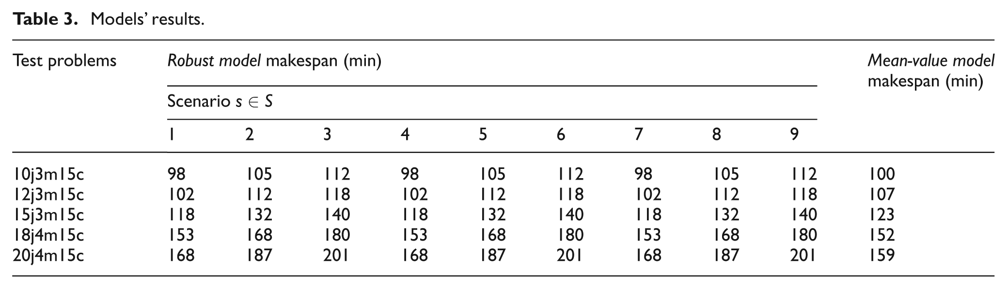
A commercial optimization solver, the CPLEX, embedded in GAMS 23.8 is used to solve the problem instances. In Table 3, the resulting makespan’s value for both mean-value and robust models (in each probable scenario) is considered in which the values of ω and λ are assumed to be 40 and 1, respectively.

Table 3.

Models’ results.

Test problems	Robust model makespan (min)									Mean-value model makespan (min)
	Scenario $s \in S$
	1	2	3	4	5	6	7	8	9
10j3m15c	98	105	112	98	105	112	98	105	112	100
12j3m15c	102	112	118	102	112	118	102	112	118	107
15j3m15c	118	132	140	118	132	140	118	132	140	123
18j4m15c	153	168	180	153	168	180	153	168	180	152
20j4m15c	168	187	201	168	187	201	168	187	201	159

Trade-off between solution robustness and model robustness

Solution robustness means being near to optimality while model robustness means being less infeasible in all realizations of the scenarios. In this problem, the trade-off is between the value of makespan (solution robustness) and the number of rejected jobs (model robustness) and can be considered by changing the value of ω (last term in objective function (26)). Also, λ is considered as the weight of the variance of objective function in all scenarios (second term in objective function). These weights are relative and by increasing one weight, the other one would be affected. Therefore, decision-makers mostly change one parameter (for instance, ω) to have the aforementioned trade-off. While the decision-makers intend to have a less infeasibilities, by increasing ω the achieved solution would be more feasible in all scenarios. By decreasing ω, the outcome remains near to its optimality while the number of infeasibilities may increase. These parameters can be represented as the risk attitude of the decision-maker. As mentioned before, by means of penalty $(δ_{s})$ in control constraint (30), the robust optimization allows infeasibility in different scenarios. As shown in the second column of Table 4, by decreasing ω value, the objective function of the model decreased, but the next columns demonstrate that the number of infeasible batches and the embedded jobs in these batches will consequently increase.

Table 4.

Sensitivity analysis on different values of parameter ω.

ω	Model result (min)	Number of rejected jobs						TPR
		Scenario $s \in S$			Mean objective function value in realization (min)
		7, 8, 9	4, 5, 6	1, 2, 3	7, 8, 9	4, 5, 6	1, 2, 3
50	135	0	0	0	132	132	132	132
40	131	0	0	0	131	131	131	131
30	129	4	0	0	186	129	129	146.1
20	127	6	0	0	176	127	127	141.7
10	116.5	11	8	0	175	169	116	157.55
5	101.3	13	13	13	170	173	149	166.1
1	92	13	13	13	165	168	145	161.35

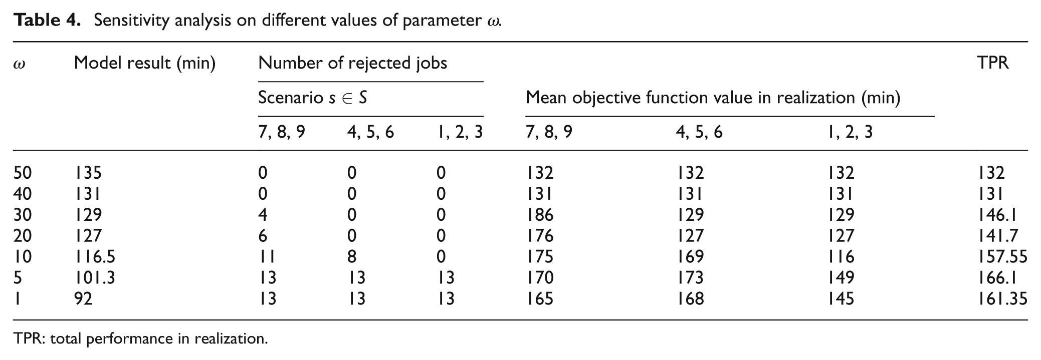
TPR: total performance in realization.

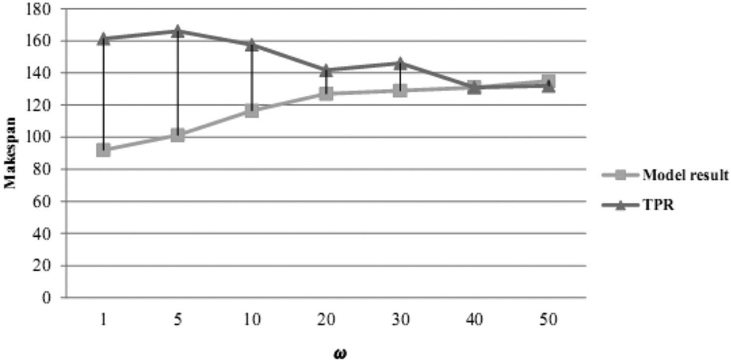
For the sake of more appropriate decision-making for ω value, the solutions obtained by different values of ω are compared in realization by Monte Carlo simulation method. The achieved simulation results for total performance in realization (TPR) are exhibited in Figure 4. Moreover, Table 4 shows that in our case, for higher values of ω, for instance, 50 and 40, better solution performance in realization can be obtained, and rejected jobs cause some increases in value of makespan in realization. In addition, by increasing the value of ω, the gap between real performance and model result decreased.

Figure 4.

Sensitivity analysis on value of parameter ω.

Comparing effectiveness of robust optimization model

For the purpose of demonstrating the effectiveness of the suggested scenario-based robust scheduling model, a comparative analysis for the performance of both the MVM and the robust model based on Monte Carlo simulation method was done. It was aforementioned that the MVM exploits the mean values, regardless to the inherent uncertainty of parameters, but in the proposed model, the intrinsic uncertainties were also considered such as processing time and job sizes.

Obviously, the derived makespan for MVM in Table 3, just in occurrence of scenario 5, is achievable, and in realization of other scenarios some changes in value of makespan are anticipated. In Table 4, the percentage of infeasible iteration in simulation is shown and it is worthy to know that just in occurrence of scenarios 7, 8, and 9, MVM’s solution can violate the capacity limitation of machines’ capacity.

Table 5 demonstrates that in infeasible iteration of simulation, how many numbers of batches and jobs violated the machines’ capacity constraint; as mentioned in section “Problem description,” these jobs should be grouped, batched, and scheduled again. Furthermore, Table 5 compares the performance of MVM and robust model in scenarios 7, 8, and 9, in which infeasible iterations happened by MVM’s solution and can be understood that performance of robust model is much better than MVM.

Table 5.

Results of simulation in realization of scenarios 7, 8, and 9 for both MVM and RM.

Test problems	Number of rejected batch (MVM)	Number of rejected jobs (MVM)	Mean objective function of RM (min)	Objective function MVM (min)
10j3m15c	1	3	105	159
12j3m15c	2	6	112	170.5
15j3m15c	2	8	132	185
18j4m15c	4	15	168	219
20j4m15c	5	17	187	244.8

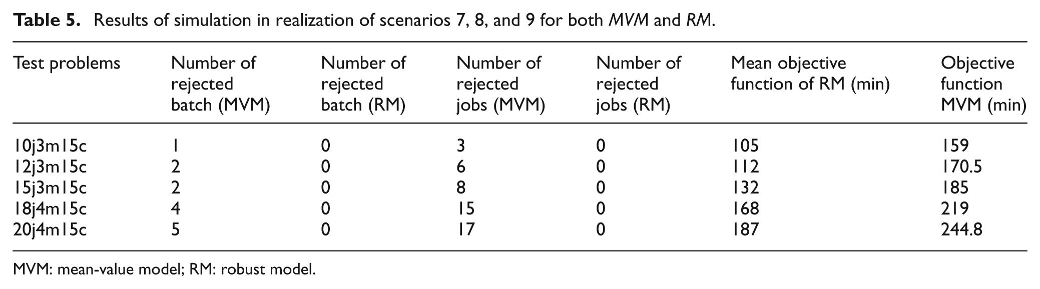
MVM: mean-value model; RM: robust model.

In Table 6, the derived mean value for objective function of MVM and robust model within all simulation iterations is demonstrated. The total performance of the mentioned models can be compared with each other, and as depicted in Figure 5, the performance of robust model is better than MVM in all test problems. This could be verified using a Student’s t-test and the results are summarized in Table 7 where the obtained p value rejects the null hypothesis. In the plain language, there is a significant difference between the two methods at the 5% level in which means the robust model has a better performance than MVM in realization.

Table 6.

Total performance of RM and MVM.

Test problems	10j3m15c	12j3m15c	15j3m15c	18j4m15c	20j4m15c
RM (min)	105	112	132	168	187
MVM (min)	120.5	130.5	147	186.5	205

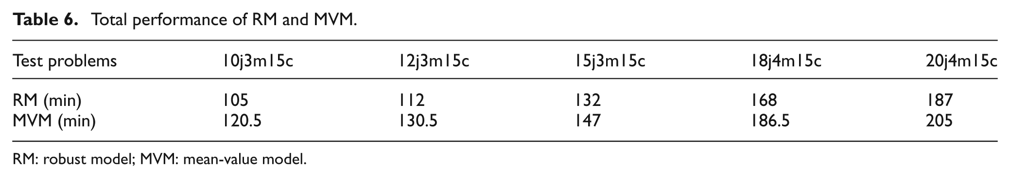
RM: robust model; MVM: mean-value model.

Figure 5.

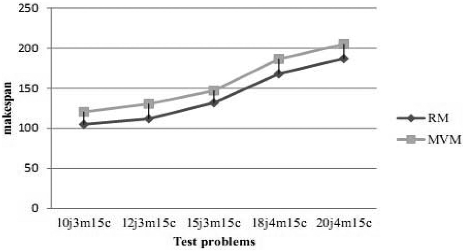
Total performance realization of mean-value model (MVM) versus robust model (RM) in different test problems.

Table 7.

Paired t-test: RM versus MVM.

	Mean	Std deviation	Std error mean	95% Confidence interval of the difference		T	d.f.	p value
	Mean	Std deviation	Std error mean	Lower	Upper	T	d.f.	p value
RM–MVM	−17.1	1.710	0.7648	−19.22	−14.97	−22.3	4	0.000

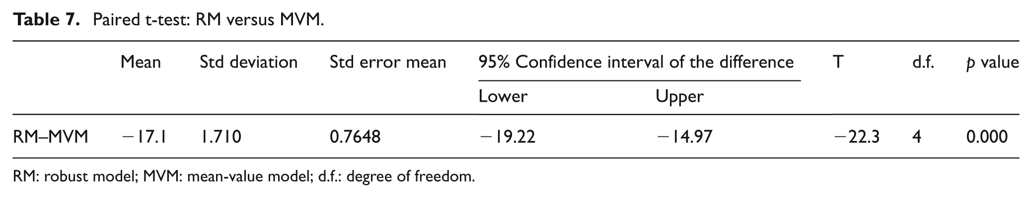
RM: robust model; MVM: mean-value model; d.f.: degree of freedom.

Conclusion

This study developed a scenario-based optimization approach for a real-world flow shop problem with any number of BPMs that the processing time and size of jobs are uncertain. Each machine can process multiple jobs simultaneously as long as the machine capacity is not violated. In order to verify the developed mathematical model and evaluate the performance of proposed robust counterpart, a number of test problems are generated and a commercial optimization solver, the CPLEX embedded in GAMS 23.8, is used to solve the test problem. For the purpose of analysis on the results, the robust model and MVM were tested through a Monte Carlo simulation method. The simulations results demonstrate that the MVM and low value of ω make many infeasible solutions. In contrast, high values of ω have better performance in realization.

For further research, because the model is non-deterministic polynomial-time (NP-hard), it is recommended to apply metaheuristic algorithms so as to solve the large-scale problems.

Footnotes

Declaration of conflicting interests

The authors declare that there is no conflict of interest.

Funding

This research received no specific grant from any funding agency in the public, commercial, or not-for-profit sectors.

References

Noroozi

Mokhtari

Kamal Abadi

INK

. Research on computational intelligence algorithms with adaptive learning approach for scheduling problems with batch processing machines. Neurocomputing 2013; 101: 190–203.

Lin

Y-K

Chang

P-C

. Reliability of a production system with intersectional lines. Proc IMechE, Part B: J Engineering Manufacture. Epub ahead of print 24 June 2013. DOI: 10.1177/0954405413486463.

Damodaran

Srihari

. Mixed integer formulation to minimize makespan in a flow shop with batch processing machines. Math Comput Model 2004; 40: 1465–1472.

Chou

F-D

. A joint GA+ DP approach for single burn-in oven scheduling problems with makespan criterion. Int J Adv Manuf Tech 2007; 35: 587–595.

Chou

F-D

Wang

H-M

. Scheduling for a single semiconductor batch-processing machine to minimize total weighted tardiness. J Chin Inst Ind Eng 2008; 25: 136–147.

Damodaran

Srihari

Lam

. Scheduling a capacitated batch-processing machine to minimize makespan. Robot Cim-Int Manuf 2007; 23: 208–216.

Heywood

Chan

Chatwin

. Application of stochastic real-valued reinforcement neural networks to batch production rescheduling. Proc IMechE, Part B: J Engineering Manufacture 1997; 211: 591–603.

Kashan

Karimi

. Scheduling a single batch-processing machine with arbitrary job sizes and incompatible job families: an ant colony framework. J Oper Res Soc 2008; 59: 1269–1280.

Kashan

Karimi

Jolai

. Effective hybrid genetic algorithm for minimizing makespan on a single-batch-processing machine with non-identical job sizes. Int J Prod Res 2006; 44: 2337–2360.

10.

Melouk

Damodaran

Chang

P-Y

. Minimizing makespan for single machine batch processing with non-identical job sizes using simulated annealing. Int J Prod Econ 2004; 87: 141–147.

11.

Dauzère-Pérès

Mönch

. Scheduling jobs on a single batch processing machine with incompatible job families and weighted number of tardy jobs objective. Comput Oper Res 2013; 40: 1224–1233.

12.

Mazumdar

Mathirajan

Gopinath

. Tabu search methods for scheduling a burn-in oven with non-identical job sizes and secondary resource constraints. Int J Oper Res 2008; 3: 119–139.

13.

Mönch

Unbehaun

Choung

. Minimizing earliness—tardiness on a single burn-in oven with a common due date and maximum allowable tardiness constraint. OR Spectrum 2006; 28: 177–198.

14.

Griffiths

Dimov

Fischer

. Micro-stereolithography tools for small-batch manufacture of polymer micro-parts. Proc IMechE, Part B: J Engineering Manufacture. Epub ahead of print 13 December 2011. DOI: 10.1177/0954405411429242.

15.

Jiang

. A memetic algorithm approach for batch-model assembly line balancing problem of sub-block in shipbuilding. Proc IMechE, Part B: J Engineering Manufacture. Epub ahead of print 23 January 2014. DOI: 10.1177/0954405413518511.

16.

Chang

P-Y

Damodaran

Melouk

. Minimizing makespan on parallel batch processing machines. Int J Prod Res 2004; 42: 4211–4220.

17.

Damodaran

Hirani

Vélez-Gallego

. Scheduling identical parallel batch processing machines to minimise makespan using genetic algorithms. Eur J Ind Eng 2009; 3: 187–206.

18.

Damodaran

Vélez-Gallego

. Heuristics for makespan minimization on parallel batch processing machines with unequal job ready times. Int J Adv Manuf Tech 2010; 49: 1119–1128.

19.

Damodaran

Vélez-Gallego

. A simulated annealing algorithm to minimize makespan of parallel batch processing machines with unequal job ready times. Expert Syst Appl 2012; 39: 1451–1458.

20.

Malve

Uzsoy

. A genetic algorithm for minimizing maximum lateness on parallel identical batch processing machines with dynamic job arrivals and incompatible job families. Comput Oper Res 2007; 34: 3016–3028.

21.

Mönch

Balasubramanian

Fowler

. Heuristic scheduling of jobs on parallel batch machines with incompatible job families and unequal ready times. Comput Oper Res 2005; 32: 2731–2750.

22.

Wang

H-M

Chou

F-D

. Solving the parallel batch-processing machines with different release times, job sizes, and capacity limits by metaheuristics. Expert Syst Appl 2010; 37: 1510–1521.

23.

Shukla

Tiwari

. Integrated model for the batch sequencing problem in a multi-stage supply chain: an artificial immune system based approach. Int J Prod Res 2009; 47: 1015–1037.

24.

Chan

FTS

. The effects of scheduling flexibility on the performance of a flexible manufacturing system. Proc IMechE, Part B: J Engineering Manufacture 2003; 217: 899–918.

25.

Rahmani

Heydari

. Robust and stable flow shop scheduling with unexpected arrivals of new jobs and uncertain processing times. J Manuf Syst 2014; 33: 84–92.

26.

Verderame

Elia

. Planning and scheduling under uncertainty: a review across multiple sectors. Ind Eng Chem Res 2010; 49: 3993–4017.

27.

Kouvelis

Kurawarwala

Gutierrez

. Algorithms for robust single and multiple period layout planning for manufacturing systems. Eur J Oper Res 1992; 63: 287–303.

28.

Lawler

Lenstra

Rinnooy Kan

. Sequencing and scheduling: algorithms and complexity. Amsterdam: Elsevier, 1989.

29.

Daniels

Kouvelis

. Robust scheduling to hedge against processing time uncertainty in single-stage production. Manage Sci 1995; 41: 363–376.

30.

Rossi

. A robustness measure of the configuration of multi-purpose machines. Int J Prod Res 2010; 48: 1013–1033.

31.

Jensen

. Generating robust and flexible job shop schedules using genetic algorithms. IEEE T Evolut Comput 2003; 7: 275–288.

32.

Bouyahia

Bellalouna

Jaillet

. A priori parallel machines scheduling. Comput Ind Eng 2010; 58: 488–500.

33.

Al-Fawzan

Haouari

. A bi-objective model for robust resource-constrained project scheduling. Int J Prod Econ 2005; 96: 175–187.

34.

Chtourou

Haouari

. A two-stage-priority-rule-based algorithm for robust resource-constrained project scheduling. Comput Ind Eng 2008; 55: 183–194.

35.

Raja

Selladurai

Saravanan

. Earliness—tardiness scheduling on uniform parallel machines using simulated annealing and fuzzy logic approach. Proc IMechE, Part B: J Engineering Manufacture 2008; 222: 333–346.

36.

Mulvey

Vanderbei

Zenios

. Robust optimization of large-scale systems. Oper Res 1995; 43: 264–281.

37.

C-S

H-L

. A robust optimization model for stochastic logistic problems. Int J Prod Econ 2000; 64: 385–397.

A scenario-based robust optimization approach for batch processing scheduling

Abstract

Keywords

Introduction

Scenario-based robust optimization

Problem description

Notations of the model

Sets

Parameters

Decision variables

Dependent variables

MVM for BPM’s scheduling problem

Robust model for BPM’s scheduling

Experimental results

Trade-off between solution robustness and model robustness

Comparing effectiveness of robust optimization model

Conclusion

Footnotes

Declaration of conflicting interests

Funding

References