
Abstract
This article integrates the company operations decisions (i.e. location, production, inventory, distribution, and transportation) and finance decisions (i.e. cash, accounts payable and receivable, debt, securities, payment delays, and discounts) in which the demands and return rate are uncertain, defined by a set of scenarios. The cash flow and budgeting model will be coupled with supply chain network design using a mixed integer linear programming formulation. The article evaluates two financial criteria, that is, the change in equity and the profit as objective functions. The results indicate that objective functions are partially interdependent, that is, they conflict in certain parts. This fact illustrates the inadequacy of treating process operations and finances in isolated environments and pursuing objective myopic performance indicators such as profit or cost. Due to the importance of the supply chain network design problem, a multi-objective robust optimization with the max–min version is extended to cope with the uncertainty. A solution approach integrating Benders’ decomposition method with the scenario relaxation algorithm is also proposed in this research. The improved algorithm has been applied to solve a number of numerical experiments. All results illustrate significant improvement in computation time of the improved algorithm over existing approaches. For a problem, the proposed algorithm shows a significant reduction in computational time compared with the Benders’ decomposition and scenario relaxation that shows the efficiency of the proposed solution method.
Keywords
Introduction
Nowadays, most companies address the company operations decisions and financial issues in isolated environments and optimize partial sets of decision variables. Therefore, although they enhance the share of information between different businesses, in the manner that each functional area’s plan provides input parameters for the computation of other related business decisions according to a hierarchy, they do not lead to real integration relationships. Supply chain management (SCM) models are often focused on the physical flows of goods in a network, including the best location of facilities, the optimum flow of materials/products and optimum value of inventory with respect to the performance measure of cost or profit. The examples of models and solution procedures for SCM problems can be found in Chan et al., 1 Gümüs and Güneri, 2 and Lee. 3 Moreover, any supply chain (SC) has in parallel a financial chain, and aspects related to the analysis of corporate financial decisions are not considered within these models. Therefore, these models are no longer adequate and must present an optimized plan along with an optimized budget. 4
Due to the problem of global warming, in particular, growing attention has been recently given to reverse logistics that refers to activities dedicated to the collection, repair, recovery, recycling, and/or disposal of the returned products within SCM. In addition, due to the fact that designing the forward and reverse logistics separately results in sub-optimal designs with respect to objectives of the SC, the design of forward and reverse logistics should be integrated. Whereas designing the forward and reverse logistics separately results in sub-optimal designs with respect to objectives of the SC, the closed-loop supply chain (CLSC) network design is critically important and can guarantee the least waste of materials by following the conservation laws during the life cycle of the materials. 5
Based on the aforementioned discussions, this article presents a model for CLSC network design integrating the physical and financial flows with the uncertainty in demands and return rate. The main contribution of this article is to incorporate the financial issues and a set of budgetary constraints representing balances of cash, debt, securities, payment delays, and discounts in the SC planning. The article evaluates two financial criteria, that is, the change in equity and the profit as objective functions. Due to the importance of the supply chain network design (SCND) problem, the robust optimization with the max–min version is extended to cope with the uncertainty. A solution approach integrating Benders’ decomposition method with the scenario relaxation algorithm is also proposed in this research.
The structure of this article is as follows. Section “Literature review” reviews the literature of the SCND problem with a focus on financial issues. A mathematical model for the design of CLSC under uncertainty with the financial considerations is presented in Section “Model formulation.” Section “Solution approach” addresses solution methodology to solve the presented model. Section “Computational results” illustrates the numerical examples and discusses the computational results. Finally, we report the conclusions of this article in Section “Conclusion.”
Literature review
In this section, we inquire into the literature and categorize studies into two cases including the studies considering the financial decisions in SCM and the researches associated with CLSC design.
Financial issues in SCM
Incorporation of financial decisions in SCM, both qualitative and quantitative studies, can be observed in the literature. Wang et al. 6 address a facility location problem with budget constraints in which the opening of new facilities and the closing of existing facilities are considered. The objective of the model is to minimize the distance from customer subject to the restriction of investment budget and number of facilities. Badell et al. 7 presented a mixed integer linear programming (MILP) model to implement the financial cross-functional links with the enterprise value-added chain, where the activities of planning, scheduling, and budgeting are integrated at plant level. The main contribution of this article is to incorporate the financial issues (i.e. budgeting model) into advanced planning and schedule (APS) enterprise systems. Guillén et al. 8 presented a mathematical model that simultaneously optimizes activities of scheduling, production planning, and corporate financial planning in a holistic framework. The objective of this article is to maximize change in equity instead of maximizing profit.
Puigjaner and Guillén-Gosálbez 9 addresses the SC optimization at the operation level in the chemical process industry. An integrated approach is suggested for SCM in a multi-agent framework. The article considers SC dynamics, the environmental impacts, the business issues, and a key performance indicator in the proposed problem. Hammami et al. 10 presented a strategic-tactical model for the design of a SC network in the delocalization context. The article considers the logistic decisions, that is, location of facilities, technology choice, supplier selection, and product flows among chain, as well as the financial decisions, that is, transfer pricing and transportation costs allocation. Laínez et al. 11 presented a model for SCM with a focus on the process operations and the product development pipeline management (PDPM) problem. The article addresses the financial and financial engineering considerations with inflow and outflow cash in each period, strategic management of supplier and customer relations by inventory management and option contracts. Protopappa-Sieke and Seifert 12 presented a mathematical model to integrate the operational and financial SCM in the inventory control area. The model decides on the optimal purchasing order quantity with respect to the capital constraints and payment delays while performance measurements of the service level, return on investment, profit margin, and inventory level are analyzed in the relevant SC. Longinidis and Georgiadis 13 proposed a MILP formulation for design of a SC network, including plants, warehouses, distribution centers, and customers. The article extends the existing models in the literature by incorporating the financial issues as financial ratios and considering the demand uncertainty.
CLSC design
In the second stream, network design in CLSC, various studies have addressed this problem in the literature. Chan et al. 1 presented a facility location–allocation model for collection, reprocessing, and redistribution of carpets to design the location and capacity of a regional recovery center. The model minimized the costs of investment, processing, and transportation. Fleischmann et al. 5 proposed a SCND model analyzing the forward flow together with the return flow. Fleischmann’s model was extended by Salema et al. 14 to a multi-product capacitated reverse logistic network with uncertainty in the demands and returns, which was used by an Iberian company. Üster et al. 15 presented a multi-product closed-loop SCND model considering the production and reproduction separately. They considered the feature of single sourcing for the customers to better manage the customers. The Benders’ decomposition method was also used to solve the model. Chan et al. 1 simulated a carpet reverse logistic network. The article also analyzed the effect of the system design and the environmental factors on the operational performance of the reverse logistic system.
Ko and Evans 16 developed a dynamic, integrated, closed-loop network operated by the third-party logistics (3PL) service provider. They applied a genetic algorithm (GA) to solve their model. Aras et al. 17 presented a non-linear recovery logistic network design the objective of which is to maximize the total profit. The model made decisions about the locations of collection centers and suitable prices for returned products. Moreover, a Tabu search solution procedure was proposed to find the solution of the model. Min and Ko 18 proposed a dynamic design of a reverse SCND problem and presented a GA to solve the problem, including the location and allocation for 3PLs. Salema et al. 19 introduced a multi-product and multi-period model for a SC network with reverse flows, where an approach based on the graph is applied to model the relevant problem. The model simultaneously integrates the strategic decisions (i.e. network design) and the tactical decisions (i.e. planning of SC related to supply, production, storage, and distribution). El-Sayed et al. 20 proposed a multi-period, multi-echelon, forward–reverse logistics network design model. They considered four layers in the forward direction (i.e. suppliers, plants, distribution centers, and customers) and three layers in the return direction (i.e. customers, disassembly, and redistribution centers). The objective of their model is to maximize the profit of the SC.
Pishvaee et al. 21 suggested a bi-objective integrated CLSC design model, in which the costs and the responsiveness of logistic network are considered as objectives of the model. They developed an efficient multi-objective memetic algorithm by applying three different local searches in order to find the set of non-dominated solutions. Wang and Hsu 22 presented a closed-loop SCND model that takes into account the locations of plants, distribution centers, and dismantlers as decision variables. The model used the distribution centers as hybrid processing facilities for both the forward and backward flows. In addition, to solve the proposed model, a revised spanning-tree-based GA with determinant encoding representation was introduced. Ramezani et al. 23 introduced a multi-objective stochastic model to design a forward–reverse SC network under an uncertain environment. The performance of the chain is evaluated through three measures: profit, customer responsiveness, and quality of suppliers (using Six Sigma concept). The pareto-optimal solutions along with the relevant financial risk are computed to illustrate trade-offs of objectives and give a proper insight for having better decision-making.
As pointed out by Shapiro 24 and Melo et al. 25 , it can be concluded that few studies consider the financial aspects in the SCM; however, the studies integrating financial flows with physical product flows in the SCM, especially in the CLSC area, remains scarce. 26 Moreover, the majority of these studies consider the financial aspects as endogenous variables, whereas this article considers the financial aspects as exogenous variables with details that appeared in the constraints and the objective functions. Furthermore, the properties of the model such as network structure, financing sources, discount, uncertain parameters, and the solution approach differentiate this article from others in the literature.
Model formulation
The general structure of the proposed closed-loop logistic network is illustrated in Figure 1. In the forward direction, the suppliers are responsible for providing the raw material to manufacturing facilities. The new products are conveyed from plants to customers via distribution centers to meet the customer demands. In the backward direction, the returned products from customers are transferred to collection centers for testing and inspecting. After testing in collection centers, the recyclable, remanufactureable, repairable, and disposable products are shipped to suppliers, plants, repair centers, and disposal centers, respectively. The purpose is to evaluate a closed-loop logistic system with criteria of profit and the change in equity. The following sets, parameters, and variables are used in the formulation:
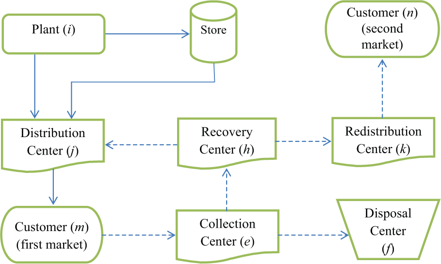
The structure of the proposed SC network.
The proposed multi-echelon closed-loop logistic network design problem can be formulated as follows
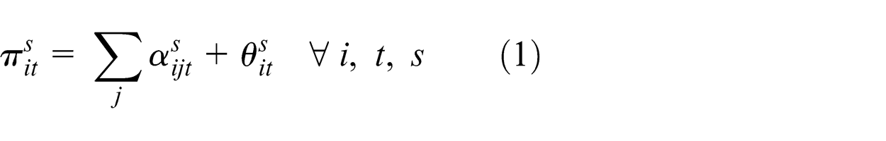
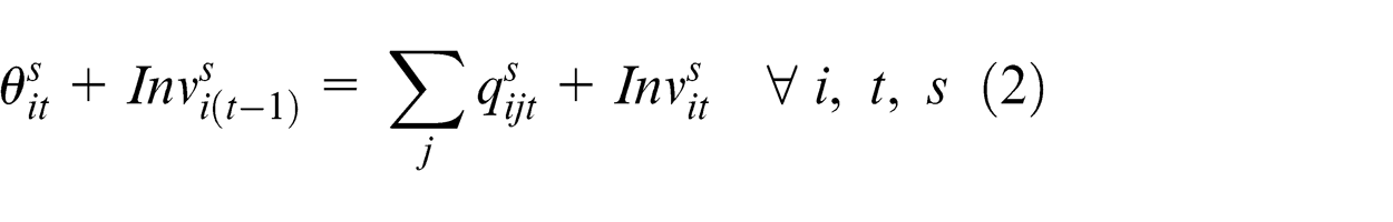
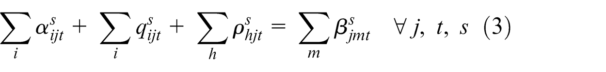
Equation (1) shows that the production value for each plant is equal to the sum of the goods flow from the plant to all distribution centers and from the plant to its store. Equation (2) shows that for each plant and in each period, the sum of the good flow from the plant to its store and the residual inventory from the previous period is equal to the sum of the good flow from the plant store to all distribution centers and the existing residual inventory. Equation (3) shows that for each distribution center and in each period, the sum of the good flow from all plants, plant stores, and recovery centers to the distribution center is equal to the sum of the good flow from the distribution center to all customers
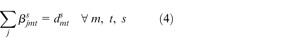
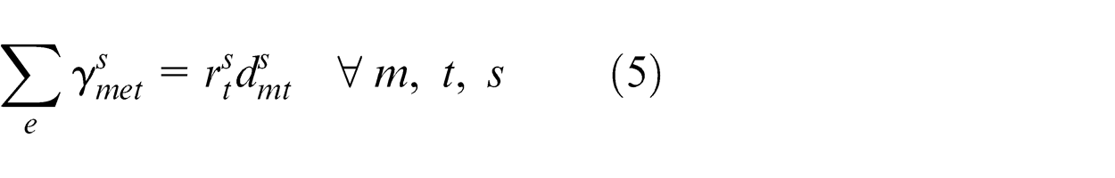
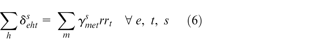
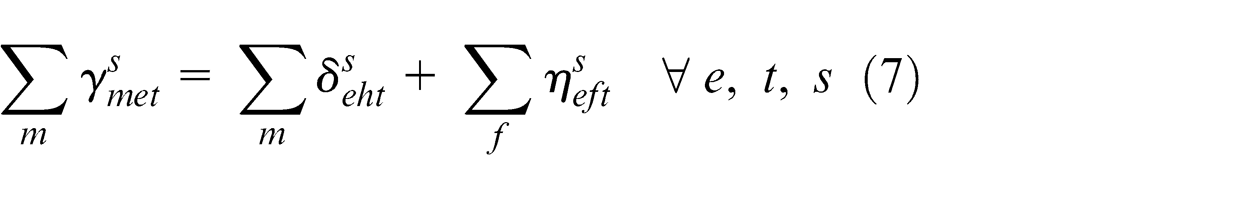
Equation (4) states that the demand of each customer must be satisfied in each period. Equation (5) relates the returned flow to the demand of customers in each period. Equations (6) and (7) show the returned flows from the collection center to the recovery and disposal centers, respectively
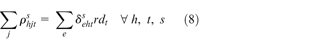
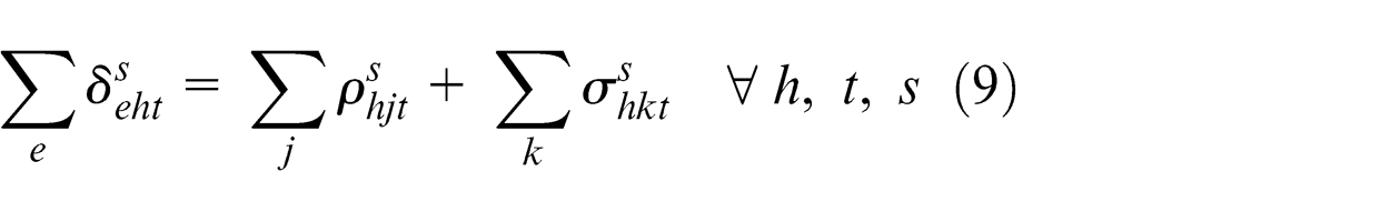
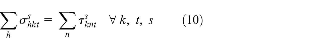
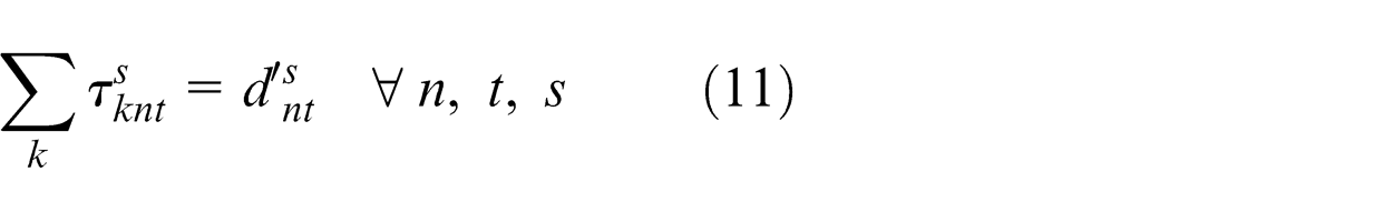
Equation (8) relates the returned flow from the collection center to the returned flow to the distribution center in each period. The constraints (9)–(11) conduct the returned flows to the redistribution centers and second customer zones
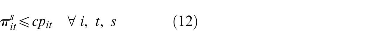
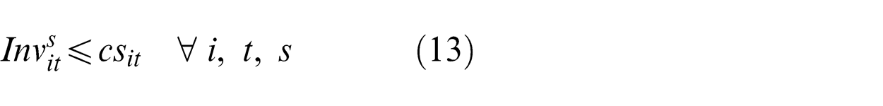
Constraint (12) restricts the production value to the capacity of the relevant plant. Constraint (13) shows the capacity of the plant store in each time period
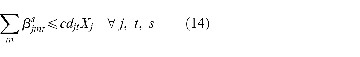
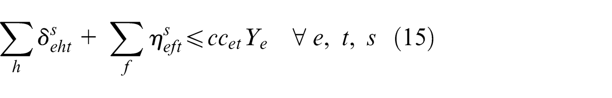
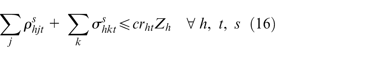
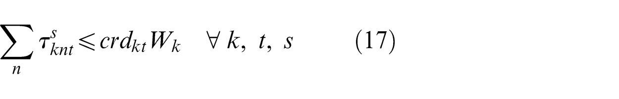
Constraints (14)–(17) show the capacity of the distribution center, collection center, recovery center, and redistribution center, respectively
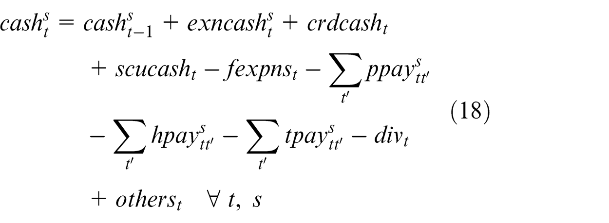
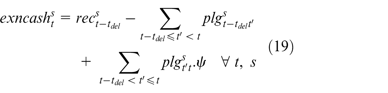
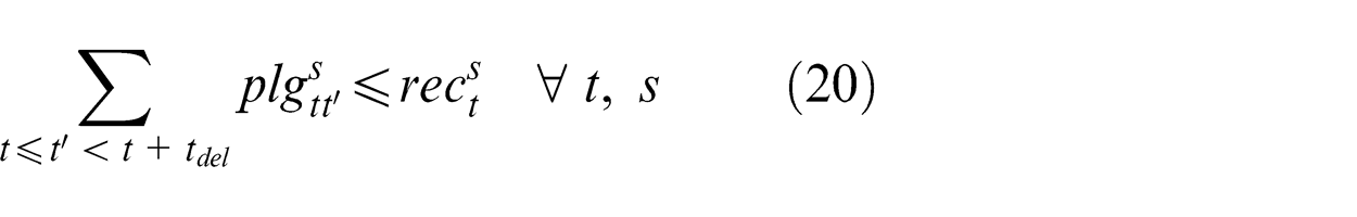
Equation (18) states that the cash in each period is computed based on the cash in the previous period, exogenous cash derived from the sales of products, and the pledging of accounts receivables, net cash obtained by money borrowed or repaid to the credit line, net cash received or paid in securities transactions, payment for costs related to facilities, dividends, and net cash resulted from any other source. Equation (19) shows that the exogenous cash in each period is equal to the sum of the receivable accounts belonging to period of
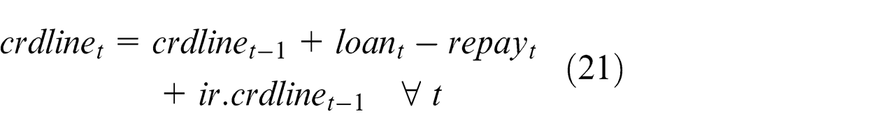

Equation (21) states that the total debt in each period is a function of the debt in the previous period, cash borrowed from the credit line, cash repaid to the credit line, and the interest costs, where net cash obtained by money borrowed or repaid to the credit line is defined as equation (22). In addition to pledging, a loan from the bank is another financing source, obtained at the beginning of a period with annual interest rate (
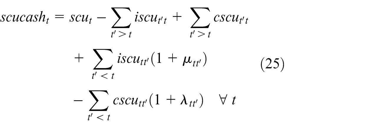

Equation (25) shows that, in each period, the cash relevant to the securities transactions is computed as the sum of the cash derived from the marketable securities of the initial portfolio, minus the cash invested as the marketable securities in the current period, plus the cash resulted from the sale of the marketable securities in the current period, plus the total cash obtained in the current period by the marketable securities invested in previous periods with regard to the technical coefficient of investment (
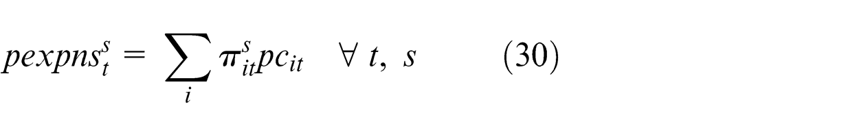
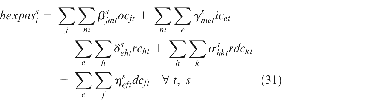
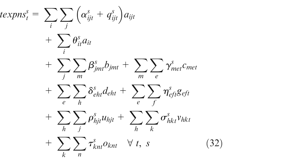
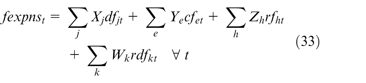
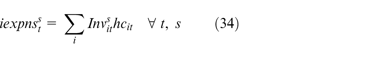
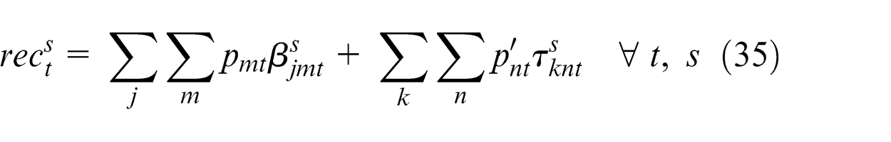
To determine the outflows of cash required to compute the profit and the equity, the expense of production, handling, transportation, establishing facilities, and holding inventory are defined as equations (30)–(34), respectively. Equation (35) shows that in each period, the accounts receivable are defined as the sale of final products to the customers in the same period
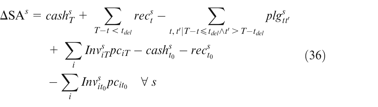
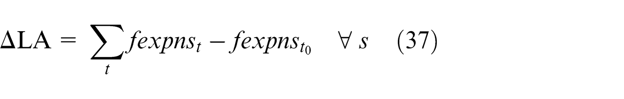
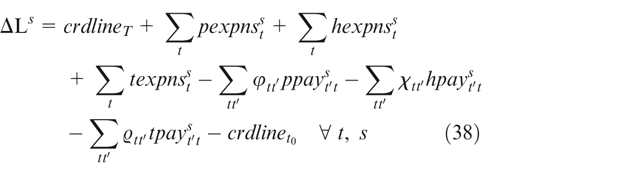
The change in short-term assets are equal to the difference between the short-term assets (including the cash available, accounts receivable, and inventory) at the end of the first period and last period presented as equation (36). In this equation, the inventory value is computed based on the generally accepted accounting principles (GAAP) of historic cost, that is, the lowest price that is the production price. Equation (37) shows the change in long-term assets as the sum of expenses of establishing facilities at the end of the last period minus the expenses of establishing facilities at the end of the first period. Equation (38) states that the change in liabilities is equal to the difference between the short-term and long-term liabilities at the end of the first period and the last period, including the debts and accounts payable related to the production, handling, and transportation
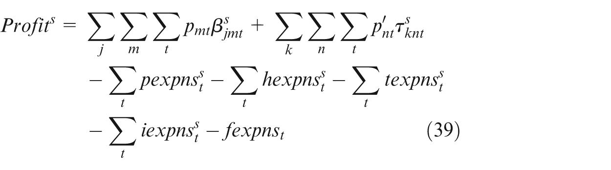
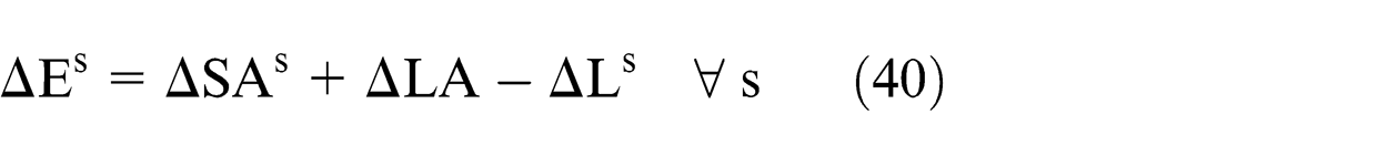
The first objective is profit that is equal to the total income associated with the sales of products in customer zones minus the total cost associated with the expenses of production, processing, inventory, and transportation expressed by equation (39). Traditionally, the decisions related to design/planning and financial issues are measured in isolated environments. The more common objectives traditionally used in the literature are maximization of the profit or minimization of the cost. However, the financial community has been making decisions for years, taking into account other criteria such as market to book value, liquidity ratios, capital structure ratios, return on equity, sales margin, turnover ratios, stock security ratios, and so on. Nevertheless, the second objective function considers the direct enhancement of the shareholder’s value as the change in equity expressed by equation (40).
Solution approach
In this section, we give details of a solution approach for solving the presented SCND problem. Our method integrates an accelerated Benders’ decomposition with the scenario relaxation algorithm.
Benders’ decomposition technique
Initialization step. Set lower and upper bounds
Step 1. Solve the master problem
s.t. Equations (21)–(23) and (25)–(26)
where
Step 2. Solve the sub-problem by fixing the solution of master problem from Step 1 for each scenario

s.t. equations (1)–(20), 24 and (27)–(35).
If the sum of objective values of Steps 1 and 2 corresponding to the current feasible solution
Step 3. If
Step 4. Update
To improve the convergence behavior of the generic Benders’ decomposition algorithm, we use a number of acceleration techniques. These strategies are described as follows.
Knapsack inequalities
Let
If a good lower bound lb is available, then adding the above knapsack inequality along with the optimality cut can have a significant impact on generating a good-quality solution from the master problem in iteration i + 1.
Upper bounding heuristics
The lower bound and solution identified in Step 2 corresponds to the solution
Step 1. Fix all the configuration decisions in the incumbent solution.
Step 2. Consider a subset of the sampled scenarios and solve the corresponding deterministic equivalent problem to solve the investment decisions.
Step 3. Evaluate the objective function corresponding to the solution (configuration and investment) obtained above by solving all the sub-problems as in Step 2. If the solution is better than
Pareto-optimal cuts
The sub-problem in Step 2 has a network sub-structure and typically such problems have multiple dual optimal solutions. Consequently, there may be alternatives for the optimality cut. While all of these alternative cuts are valid and exact at the current solution, one cut may be dominated by another in the vicinity of the optimal solution. In our implementation, we apply the Magnanti and Wong 27 strategy and consider a fractional optimal solution from the linear programming (LP) relaxation of the master problem as a candidate core point.
Valid inequalities
In the early iterations, the master problem solved in Step 1 and some valid inequalities can be added to accelerate the algorithm. We derive a set of constraints that we found to be quite useful in improving the master problem solution as follows
Multi-cut version
Since the max–min approach is considered in this study, the cut relevant to the minimum objective among sub-problems in Step 2 of the proposed Benders’ decomposition algorithm is added in each iteration. Instead, one could add all cuts relevant to other sub-problems. In this case, the master problem solved in Step 1 of the ith iteration consists of all the generated cuts. This approach can provide a better approximation and thereby improve convergence. This variant of the Benders’ decomposition algorithm is often referred to as the multi-cut version.
Scenario relaxation algorithm
Robust optimization approaches include the min–max and min–max regret versions defined by Kouvelis and Yu.
28
Let S be a finite set of scenarios and x denote the feasible solution of a given problem. For a minimization problem,
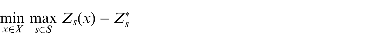
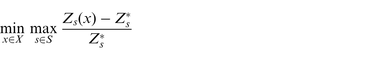
In the min–max regret version, the regret value of each scenario is defined by the difference between the objective value of the feasible solution (i.e.
Indeed, the corresponding max–min and min–max regret version can be defined for maximization problems. Aissi et al.
29
addressed the min–max regret and min–max relative regret approaches and presented a comprehensive discussion of the incentives for developing these approaches and diverse aspects of employing robust optimization in practice. Chan et al.
1
and Ben-Tal and Nemirovski
30
engaged in robust optimization, by allowing the data to be ellipsoids and proposed efficient algorithms to solve convex optimization problems under data ambiguity. Gümüs and Güneri
2
and Bertsimas and Sim
31
presented an approach for discrete optimization and network flow problems that provides the degree of conservatism of the solution to be handled. They demonstrated that the robust equivalent of an non-deterministic polynomial-time (NP)-hard
In addition, some approaches have been proposed to reduce the number of scenarios. Lee et al.
3
proposed a
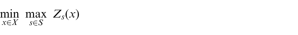
The proposed model in this study assumes that the demand and return rate are uncertain, introduced by a finite set of possible scenarios with unknown joint probability distribution. To obtain a pareto-solution of the proposed model, we use the
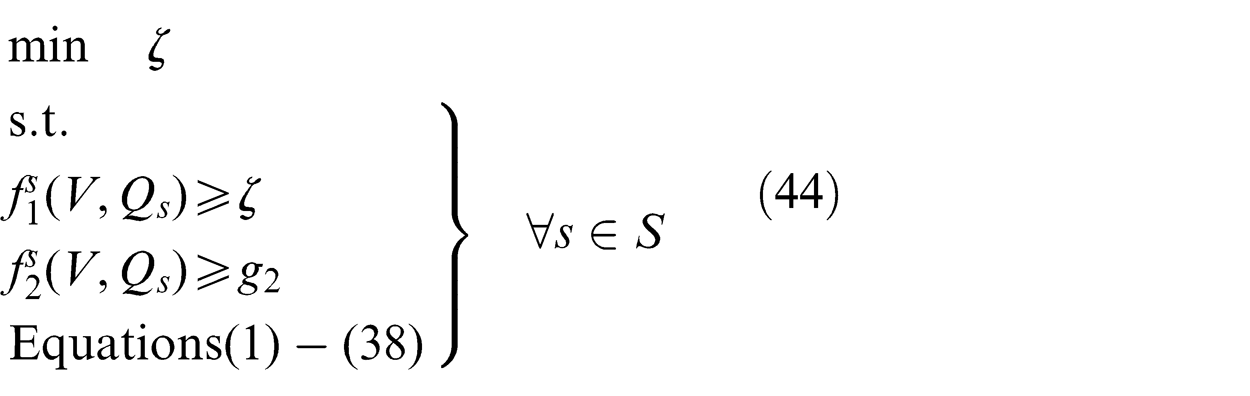
where
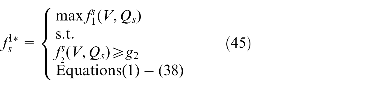
Unfortunately, the size of the model presented in equation (44), referred to as the extensive form model under deviation robust definition, can become unmanageably large when a large number of scenarios are considered. The implementation of this model requires a vigorous computational time to obtain a robust solution with a large number of scenarios. For this reason, we use the scenario relaxation algorithm to obtain a solution with a better time. In the algorithm, the optimal first objective function of each scenario is necessarily resulted by solving the following model
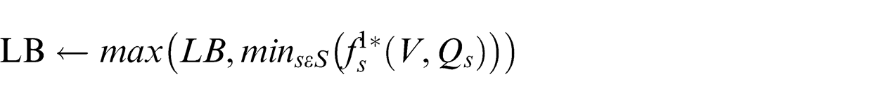
The main idea of the scenario relaxation algorithm is that in a problem with a large number of possible scenarios, only a small subset of scenarios is actually employed to find an optimal solution. Initially, the algorithm solves the problem for a subset of scenarios (sub-problems) and then sequentially searches to examine all possible scenarios. The algorithm adds those scenarios that disturb the optimality and/or feasibility conditions to the sub-problem. It is shown that the algorithm stops at an optimal robust solution (if one exists) in a finite number of iterations. 33 The overall procedure of the scenario relaxation algorithm for the max–min version can be summarized as follows
Step 0. Select a subset
Step 1. Solve the relaxed model considering only the scenario set
Step 2. Solve the general model for each scenario
Step 3. If
If
Step 4. Choose a subset
Step 5. Choose a subset
Finally, in the hybrid approach, we use the extended Benders’ decomposition algorithm in Steps 1 and 2 to solve the relaxed model and the general model.
Computational results
To demonstrate the verification and practicality, we consider several test problems to analyze the proposed SC system. The sizes of these test problems are illustrated in Table 1. The proposed CLSC involves two echelons in forward direction related to the plants, distribution centers, and first customers as well as four echelons in backward direction related to the collection centers, recovery centers, redistribution centers, disposal centers, and second customers. The plants are responsible for producing the new product to the first customer shipped via distribution centers. In the backward direction, the returned products from customers are shipped to collection centers for inspection. If the returned product is recoverable, it is shipped to the recovery center; otherwise, it is shipped to the disposal center. After shipping the recoverable products to recovery centers, depending on the quality of the recovered products, they are shipped to distribution or redistribution centers.
Size of test problems.
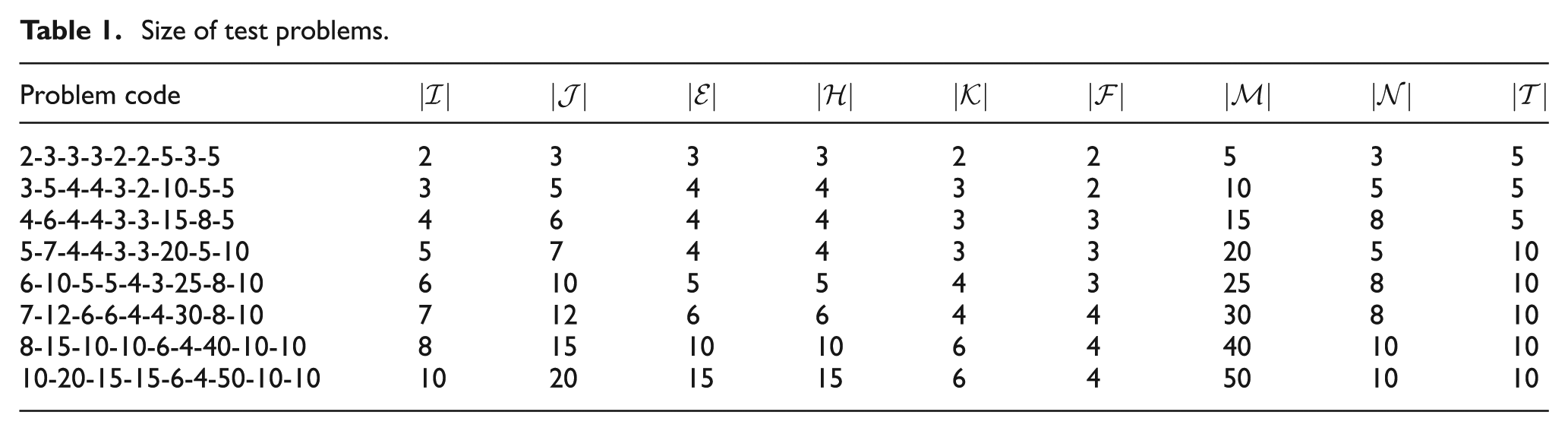
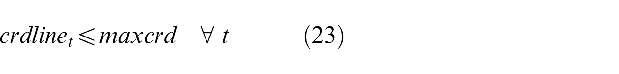
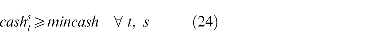
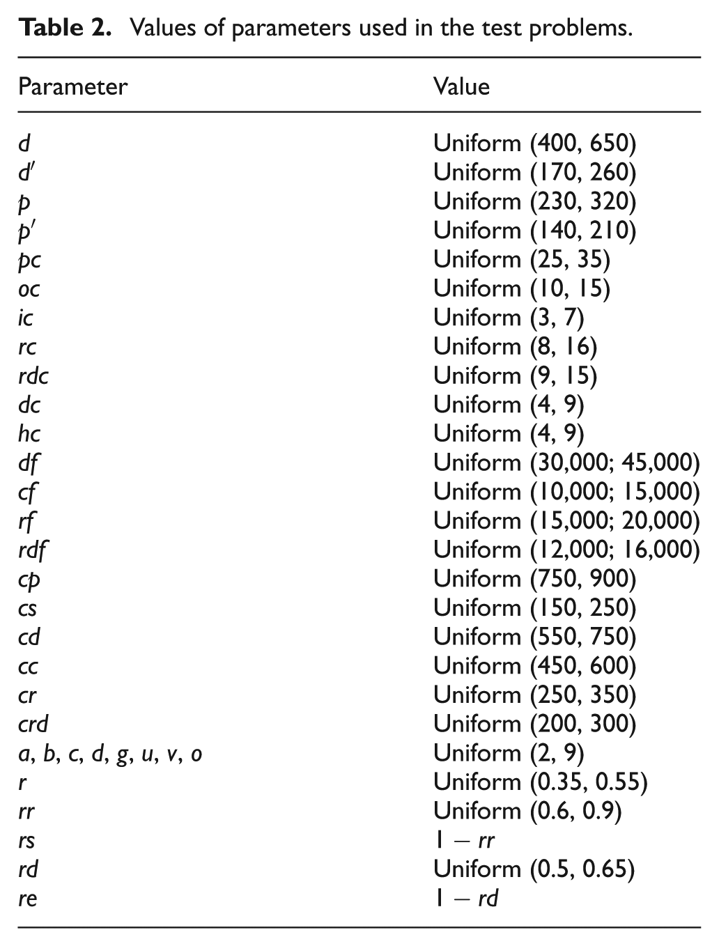
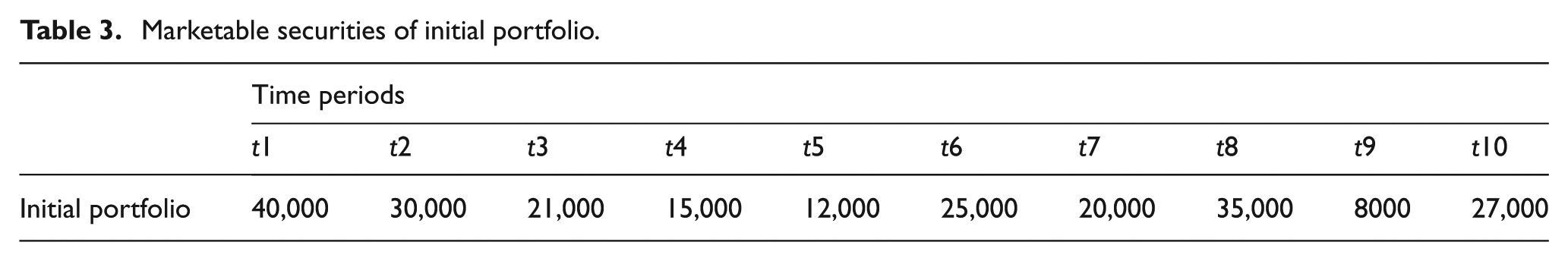
Table 2 illustrates the parameters used in the test problems. The initial cash is equal to 300,000, where the minimum cash in each period is equal to 120,000. Moreover, an open line of credit with a maximum debt of 100,000 is allowed in each period. Table 3 shows the initial portfolio of marketable securities investment. The price of the inventories at the end of the time period is the lowest price, that is, the production price. The products sold in each period are paid with a delay of two time periods, and the account receivables are pledged at 80% of their value. Moreover, liabilities borrowed due to the costs of production and processing in facilities must be repaid within three time periods (2%: one time period, net—three time periods), where technical coefficients (
Values of parameters used in the test problems.
Marketable securities of initial portfolio.
To evaluate the proposed model, first, we consider test problem 1 with Gap 0. Figure 2 shows trade-off between the profit and the change in equity as a pareto-curve, while the number of scenarios is equal to 20. As can be seen in Figure 2, the profit is decreased with an increase in the change in equity. This pareto-curve helps the DM(s) for a better analysis. Moreover, Figure 3 shows the behavior of an objective function of the change in equity under different scenarios. The value of change in equity for the robust mode computed by both the extensive model and the scenario relaxation algorithm is less than the deterministic mode, and it is reasonable because the robust approach optimizes the worst-case scenario. As can be seen in Figure 3, the values of the change in equity for the extensive model and the scenario relaxation algorithm are the same. It is proven that the scenario relaxation algorithm produces an optimal solution, of course with better time.
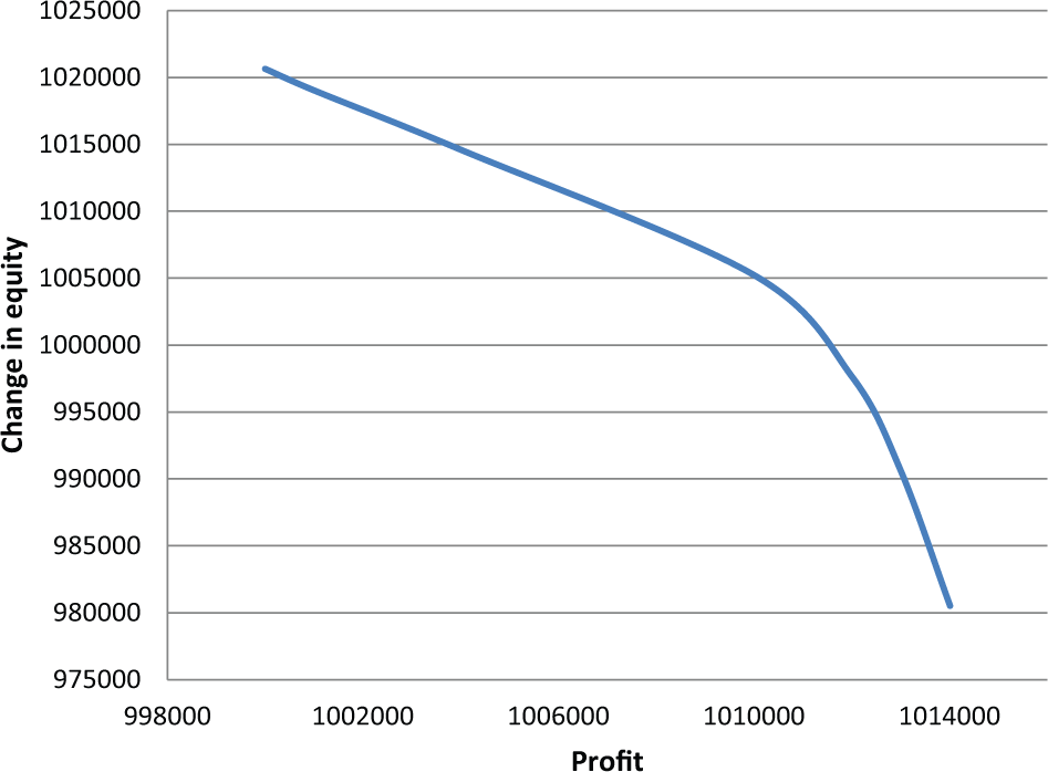
Change in equity versus profit.
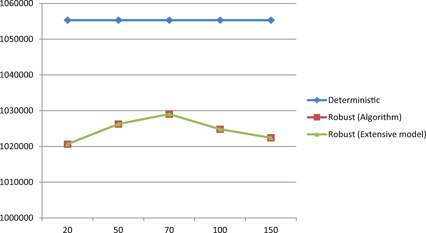
Change in equity for the different modes.
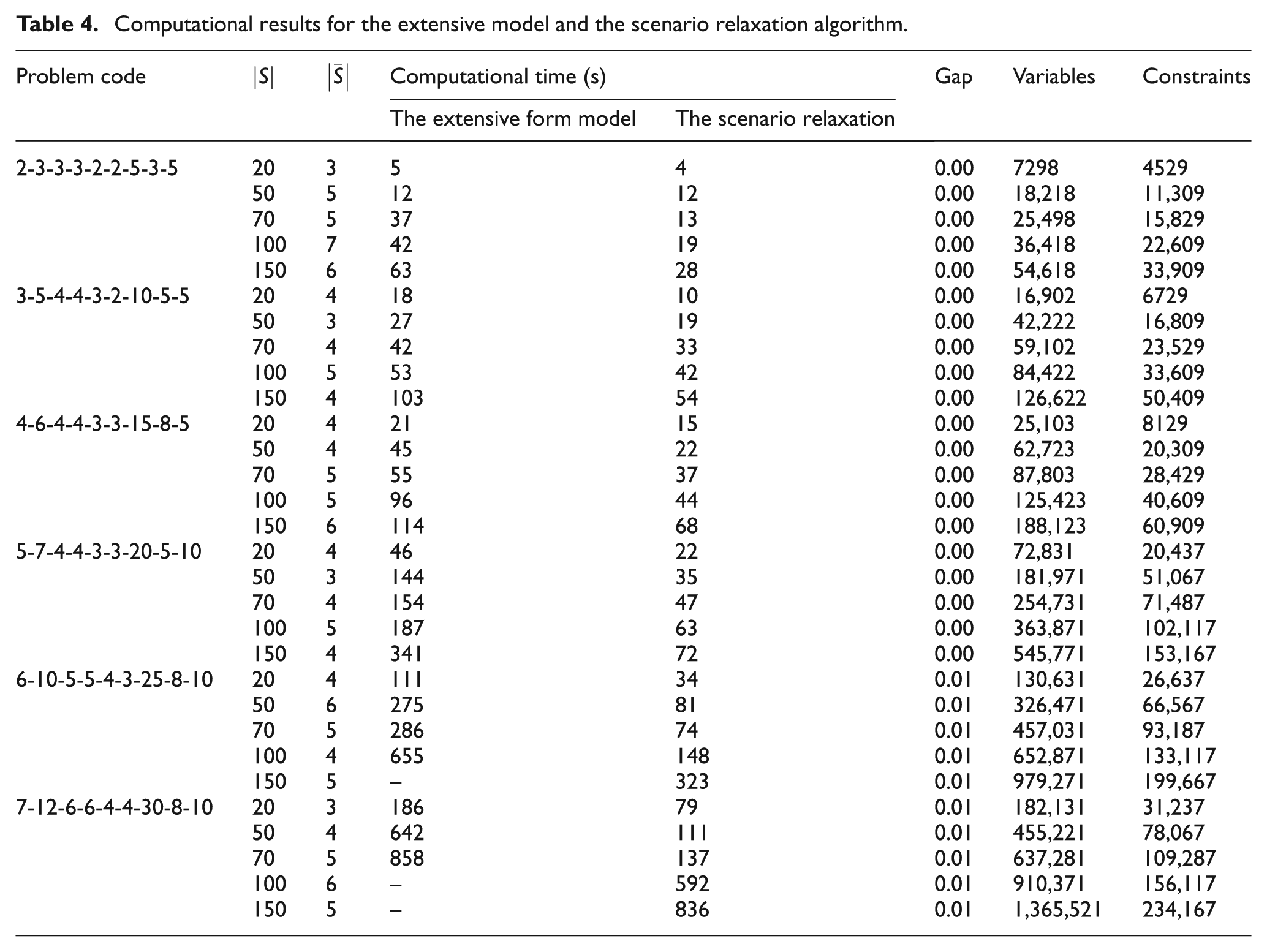
On the other hand, to illustrate the applicability of the scenario relaxation algorithm, six test problems with various scenarios are evaluated only by the change in equity, the relevant results of which are reported in Table 4. As can be observed, the number of constraints and variables of test problems increase with an increment in the number of scenarios. As the results show, the scenario relaxation algorithm dominates the extensive model in all test problems with respect to the computational time; this superiority is especially more significant when the scale of test problems and the number of scenarios are increased. Table 4 also shows the number of scenarios actually used by the scenario relaxation algorithm (i.e.
Computational results for the extensive model and the scenario relaxation algorithm.
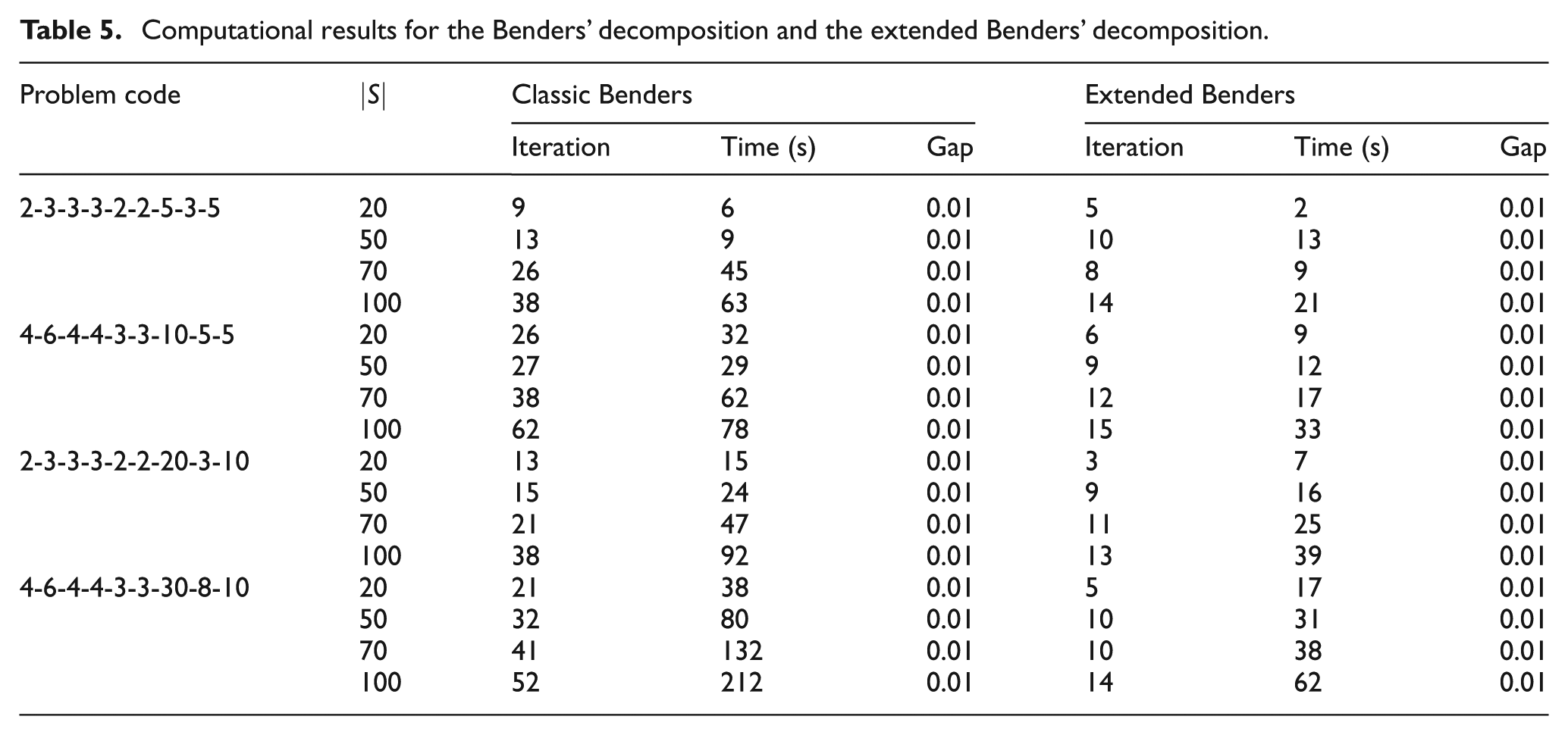
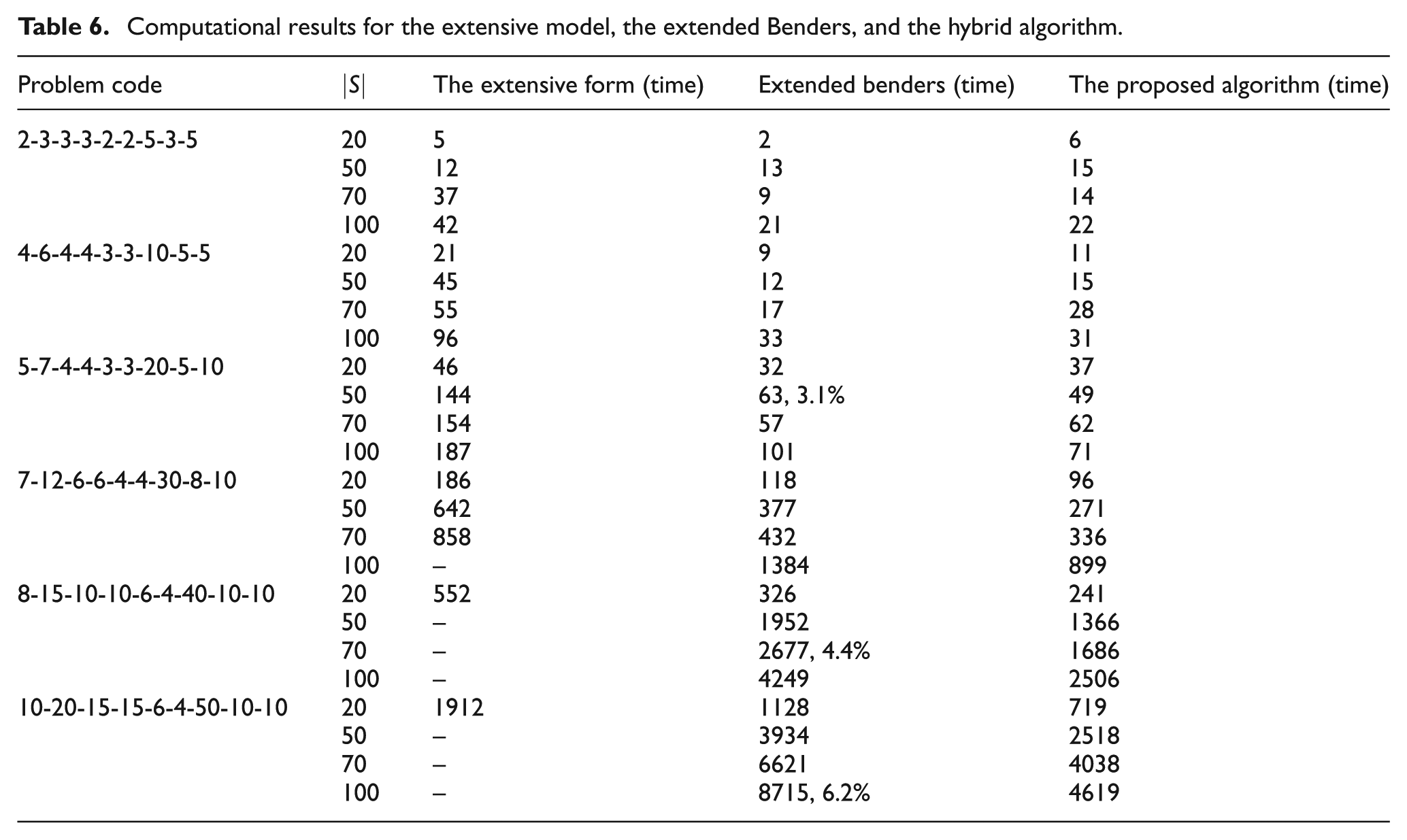
Moreover, to show the priority of the extended Benders’ decomposition compared to the classic Benders’, some test problems are considered in Table 5, where gap = 0.01. As can be seen in Table 5, the extended Benders’ decomposition has less iterations than the classic Benders due to improving the cut and adding valid inequalities. Thus, the extended Benders’ decomposition resulted in less computational time and justifies using the extension of Benders. Finally, to show efficiency of the hybrid algorithm using the scenario relaxation and the extended Benders’ decomposition, a number of test problems are considered as shown in Table 6. Table 6 compares the results of the extensive model, the extended Benders, and the hybrid algorithm. If the model does not obtain a solution within 10,000 h, the computational time is reported as “–” in this table. As can be seen, the hybrid algorithm has good performance; this superiority is especially significant when the scale of test problems and the number of scenarios are increased. According to the previous discussion, the results are consistent and obviously show the benefit of using the scenario relaxation algorithm, the extended Benders’ decomposition, and the hybrid algorithm. These results are a good improvement, which convinces the DMs employing this solution approach.
Computational results for the Benders’ decomposition and the extended Benders’ decomposition.
Computational results for the extensive model, the extended Benders, and the hybrid algorithm.
Conclusion
This study has presented a model integrating the financial flows with the physical flows in the design of a CLSC. Incorporating the financial flow helps DM(s) to make holistic decisions in order to guarantee new funds from shareholders and financial institutions that will permit the continuous financing of a company’s operations. The article has addressed an effective measure based on an economic performance indicator (the change in equity) in addition to the commonly used profit. A decision-making process that does not consider both these measures may result in a configuration that functions well only for one of the objectives while it performs poorly for other objectives. Hence, the trade-off between these measures as a pareto-curve is a useful tool for the SC managers to make a proper decision.
The model has also considered the uncertainty in the demand and return rate through a scenario, which assigns the occurring possibilities on each scenario. This approach enables the SC managers to forecast their demands and return rate as well as modify their wrong forecasts. To cope with the uncertainty, the robust optimization was implemented on the proposed model. Moreover, to find a solution with better time, a solution approach integrating Benders’ decomposition method with the scenario relaxation algorithm was also proposed in this research. Finally, it should be pointed out that other issues related to the product portfolio theory, game theory, future contracts, and sell techniques can be considered as future research.
Footnotes
Appendix 1
Declaration of conflicting interests
The authors declare that there is no conflict of interest.
Funding
This research received no specific grant from any funding agency in the public, commercial, or not-for-profit sectors.