Process modeling,joint virtual testing and construction of joint connectors for mechanical fastening by flow-drilling screws

Abstract

In this work, a computational approach is proposed in order to help establish the effect of various flow-drilling screw process and material parameters on the quality and the mechanical performance of the resulting flow-drilling screw joints. Toward that end, a sequence of three distinct computational analyses is developed. These analyses include the following: (a) finite element modeling and simulations of the flow-drilling screw process; (b) determination of the mechanical properties of the resulting flow-drilling screw joints through the use of three-dimensional, continuum finite element–based numerical simulations of various mechanical tests performed on the flow-drilling screw joints and (c) determination, parameterization and validation of the constitutive relations for the simplified flow-drilling screw connectors, using the results obtained in (b) and the available experimental results. The availability of such connectors is mandatory in large-scale computational analyses of whole-vehicle crash or even in simulations of vehicle component manufacturing, for example, car-body electro-coat paint-baking process. In such simulations, explicit three-dimensional representation of all flow-drilling screw joints is associated with a prohibitive computational cost. The approach developed in this work can be used, within an engineering-optimization procedure, to adjust the flow-drilling screw process and material parameters (design variables) in order to obtain a desired combination of the flow-drilling screw joint mechanical properties (objective function).

Introduction

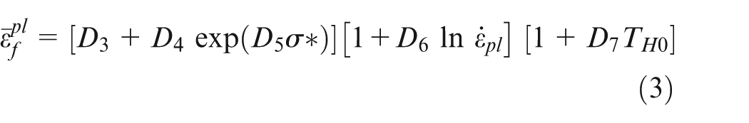
As its name implies, within the flow-drilling screw (FS) process, the holes within the workpieces to be fastened are produced by material flow/redistribution rather than by material removal.^1–3 In other words, instead of drilling out the material, the material is redistributed from the hole by a rotating and piercing steel “flow” screw into a surrounding collar/bushing. An example of a typical flow screw is depicted in Figure 1(c). It consists of the following: (a) a pointed cone-shaped tip region with a large angle (greater than 90°), (b) an adjoining smooth (either cylindrical or slightly cone-shaped) section, (c) a threaded section of a constant pitch but with an initially ramped and ultimately constant thread depth and (d) an inverted U-shaped head (shown as an inset in Figure 1(d)) designed in such a way as to accommodate the material residing in the collar (defined below).

Figure 1.

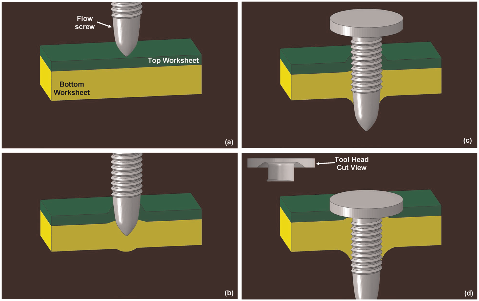
A schematic of the four basic stages of a single FS process cycle: (a) positioning, (b) piercing, (c) penetration and (d) thread engagement and final tightening.

The essence of the FS process is to bring the tip of the flow screw spinning at high speed into contact with the top workpiece, in order to generate heat (due to frictional sliding) and, in turn, soften the top (and subsequently the bottom) workpiece material(s). As the flow screw is pushed into the clamped and now thermally softened workpieces, the materials are being displaced from the generated hole into a thin collar (formed from the top workpiece material) and a bushing (formed from the bottom workpiece material). As the threaded portion of the flow screw is advanced into the clamped workpiece assembly, threads are formed within the collar/bushing, allowing a screw-type connection to be created. Close examination of the FS process reveals four distinct steps, Figure 1(a)–(d): (a) positioning, (b) piercing, (c) complete penetration and (d) thread engagement and final tightening.

Examination of the public-domain literature did not reveal many reports pertaining to the experimental characterization of either the FS process or the mechanical properties/performance of the resulting joints. The main reasons for this appear to be the following: (a) most of the work is of a proprietary type and has not been made widely accessible and (b) some of the reported work deals only with the flow-drilling portion of the FS process, that is, it does not involve the process stages associated with the formation and engagement of the threads within the collar/bushing. The reported studies most relevant to this work are briefly summarized in the following.

Miller et al. ⁴ carried out an experimental investigation of the FS process for AISI 1018 low-carbon steel workpieces. The work focused on real-time characterization of the mechanical and thermal aspects of the process. Specifically, under the condition of constant flow screw feed rate, the thrust force and torque were measured experimentally using a dynamometer. In addition, an infrared camera was utilized to monitor, in real-time, spatial distribution of the temperature over the top portion of the workpiece, as well as over the exposed portion of the flow screw. The results are used to calibrate their FS process model, the model that is subsequently used in a process optimization analysis.

Engbert et al. ⁵ explored experimentally the utility of the FS process for joining steel wire–reinforced thin-walled aluminum-extrusion profiles. These extrusion profiles are widely used for construction of frame structures, and their joining is challenging for at least two reasons: (a) their thin-walled character and (b) limited accessibility (from two sides) for joining. The work of Engbert et al. ⁵ focused on problems of forming high-integrity threads in the steel-reinforced aluminum-matrix composite extrusions, the material that is generally characterized as being “difficult-to-machine.” Specifically, the effect of steel reinforcement and the FS process parameters on the thrust force required to maintain a constant feed rate was investigated. Structural integrity of the workpiece threads, as well as of the entire FS joint, was also examined through the application of a number of mechanical testing procedures. The results obtained clearly revealed the trade-off between structural reinforcement provided to aluminum by steel wire and the quality/structural integrity of the workpiece-borne threads.

Szlosarek et al. ⁶ examined experimentally the potential of the FS process for joining dissimilar materials, specifically a top workpiece made of continuous carbon fiber–reinforced composite material and a bottom aluminum sheet workpiece. FS joints obtained under different combinations of process parameters were tested mechanically (under different loading conditions) while the testing process was recorded in real-time and analyzed for the onset and the progression of the joint damage/failure. Post-mortem microstructural/fractographic analysis was also carried out in order to identify and characterize the main modes of material damage/failure. The results obtained are used to assess the sensitivity of the load-carrying capacity, as well as of the material damage/failure mechanism, to the direction of the load applied to the joint. Furthermore, the results are used to construct a damage/failure map of the FS joint.

Examination of the public-domain literature did not reveal many reports pertaining to modeling of the FS process or the mechanical performance/properties of the FS joints. The main reason for this appears to be numerical challenges associated with modeling thread formation within the workpiece. Consequently, most of the published work related to the FS process addresses the drilling stage of this process, the stage within which the smooth portion of the flow screw interacts with the workpieces to be joined. The reported studies most relevant to this work are briefly summarized in the following.

In a two-article series by Miller et al. ⁴ and Miller and Shih, ⁷ the problem of modeling of the flow-drilling stage of the FS process has been addressed computationally. In Miller et al., ⁴ a simpler modeling approach was used to address: (a) distance traveled by the flow screw before the workpiece temperature reached a value of 250°C, the lower-bound temperature that is detectable by an infrared camera and (b) prediction of the accompanying thrust force and torque with inclusion of the effects of temperature, temperature-dependent material properties and the workpiece/flow screw contact area. Miller and Shih ⁷ extended the computational models developed by Miller et al. ⁴ as follows: (a) by analyzing the FS process through the use of a full three-dimensional (3D) finite element model and analysis; (b) the thermo-mechanical analysis employed includes an inelastic large-deformation formulation; (c) two-way mechanical/thermal coupling is achieved by having a friction-sliding/inelastic-deformation source in the thermal conduction equation, and by including temperature-dependent material properties and (d) to handle excessive mesh distortion problems, including the associated high computational cost, the following remedies are employed: (1) adaptive remeshing, (2) element deletion and (3) variable mass-scaling. A companion experimental investigation is carried out to validate/calibrate the model to match the computed/measured values for thrust force, torque and temperature (at a specific location within the workpiece).

Mathurin et al. ⁸ developed a 3D finite element model and analysis of the thread-forming stage of the FS process. Within the analysis, special attention is devoted to revealing the process of thread formation within the workpieces. A parametric study is also conducted in order to reveal the effect of FS process parameters on the thread formation mechanism and the quality/structural integrity of the resulting thread. Finally, a sensitivity analysis is carried out to identify FS process parameters having the largest effect on the structural integrity of the resulting joint.

Holmstrøm and Sønstabø ⁹ carried out a comprehensive experimental and computational investigation of the AA6061-T4 FS joints subjected to different modes of loading (e.g. normal-pull, oblique-pull, shear, in-plane shear, peel). The main objective of their modeling effort was to construct a point-to-point FS joint connector that can be used in the large-scale simulations of the FS joint automotive panels. A complete 3D modeling of such joints in full-size automotive panels is computationally prohibitive. The results obtained suggest that the constitutive relations for the point-to-point FS joint connectors can, for several (but not all) quasi-static loading modes, correctly account for the experimentally observed behavior. On the other hand, the derived connector constitutive relations quite poorly account for the experimentally measured dynamic-loading behavior, the behavior that is of primary interest under scenarios such as vehicle collision/crash.

The main objectives of this work include the following: (a) finite element modeling and simulations of the FS process; (b) determination of the mechanical properties of the resulting FS joints through the use of 3D, continuum finite element–based numerical simulations of various mechanical tests performed on the FS joints and (c) determination and parameterization of the constitutive relations for the simplified FS connectors, using the results obtained in (b) and the available experimental results. The availability of such connectors is mandatory in large-scale computational analyses of whole-vehicle crash or even in simulations of vehicle component manufacturing, for example, car-body electro-coat paint-baking process. In such simulations, explicit 3D representation of all FS joints is associated with a prohibitive computational cost.

FS process modeling

Modeling and computational analysis

Computational domain

The computational domain analyzed in this work contained two separate sub-domains, as follows: (a) an Eulerian-type sub-domain and (b) a Lagrangian-type sub-domain. The Eulerian sub-domain (which was employed to model the top and bottom worksheets to be fastened, as well as the air regions above the top worksheet and below the bottom worksheet) consisted of a parallelepiped-shaped region having dimensions of L×W×H= 17.2mm×17.2mm×15.4 mm. The mesh used for this sub-domain typically consisted of Eulerian eight-node brick elements having a characteristic dimension of 0.17 mm. The Lagrangian sub-domain was employed in the flow screw model. The flow screw geometry and size were selected in such a way as to match one of Böllhoff’s commercially available flow screws. The flow screw has been treated as a rigid body, and it was meshed using four-node tetrahedron and six-node triangular-base prismatic solid finite elements. Examples of the Eulerian and Lagrangian sub-domains analyzed in this work are shown in Figure 2(a). To help clarify the computational domain, the two worksheets, air regions and flow screw, are labeled in this figure. To aid in viewing the portion of the flow screw residing in the air region of the Eulerian domain, one quarter of the Eulerian domain has been removed in Figure 2(a). A close-up of a typical finite element mesh used in this work is shown in Figure 2(b). Typically, the Eulerian sub-domain contained approximately 1,000,000 elements while the Lagrangian flow screw domain consisted of approximately 10,000 elements. A mesh-sensitivity analysis was carried out in order to ensure that the results obtained were not very sensitive to further refinements in the mesh.

Figure 2.

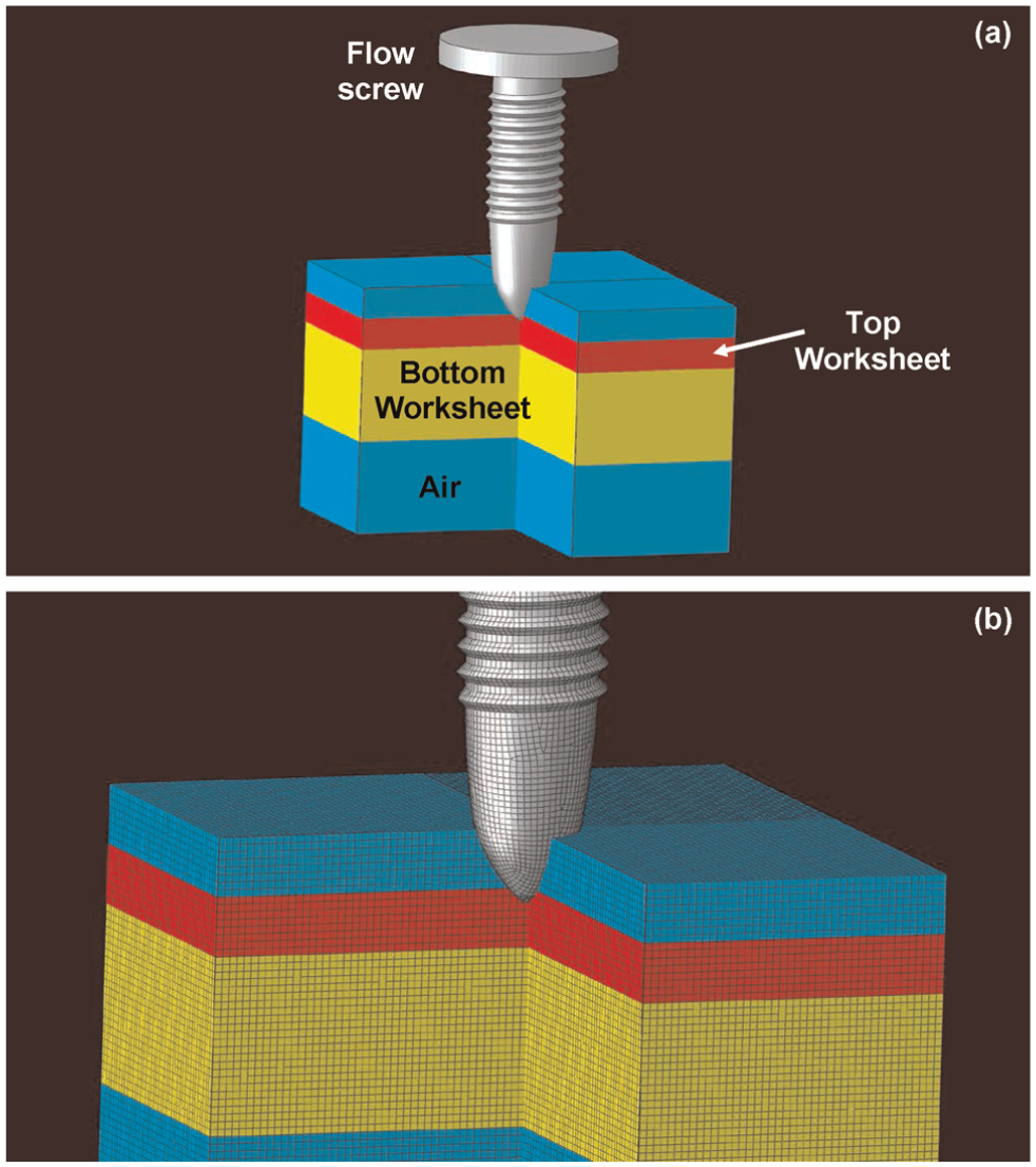
(a) Examples of the Eulerian and Lagrangian sub-domains. (b) Close-up of a typical finite element mesh used in this work.

The coordinate system used was defined as follows. The top–bottom faces of the two worksheets lay in the x–z plane and the corresponding edges were aligned with these two axes. The flow screw axis was collinear with the y-axis, with the +y-direction pointing upward.

Initial and boundary conditions

At the beginning of the analysis, a zero material velocity and stress were assigned to all the Eulerian points containing the two worksheet materials. As far as the Lagrangian sub-domain was concerned, at the start of the analysis, the flow screw was prescribed a rotational velocity (about the y-axis) and feed velocity (in the −y-direction). Additionally, ambient-temperature initial conditions were assigned to both the Eulerian and Lagrangian sub-domains.

For the Eulerian domain, zero-inflow boundary conditions were imposed over the outer faces of this domain. The size of the Eulerian computational domain in the y-direction mentioned earlier was chosen in such a way that the worksheet materials never reached the top or bottom faces of this domain (and, hence, tried to leave the domain). As far as the boundary conditions for the (rigid) flow screw were concerned, they involved a time-dependent rotational velocity (about the y-axis) and a time-dependent feed velocity (in the −y-direction) in stages 2 and 3, and a fixed torque (about the y-axis) and a fixed thrust force (in the −y-direction) in stage 4. Heat transfer from the free surfaces of the flow screw and the worksheets was assumed to be purely by convection.

Flow screw/worksheets’ contact interactions

Mesh-based surfaces could not be used to define the contact interfaces between the Eulerian and Lagrangian sub-domains, since they do not possess conformal meshes. The so-called immersed boundary method ¹⁰ was employed to determine the contact interfaces between these sub-domains. This method identifies the boundary of the Eulerian sub-domain which is occupied by the Lagrangian sub-domain during each computational time increment. A penalty method was employed to enforce Eulerian–Lagrangian contact constraints.

In addition, a kinematic constraint states that Eulerian materials within the same element must be subjected to the same strain. As a consequence of this constraint, Eulerian materials underwent “sticky” interactions with each other. Contacts between these materials allowed the transmission of normal (tensile and compressive) stresses across material boundaries, but did not allow slip at these boundaries.

Heat generation and partitioning

Two (potential) means of heat generation were considered: plastic deformation and frictional sliding. It was assumed that 95% of the plastic deformation work and 100% of the frictional sliding work were dissipated in the form of heat. Heat partitioning between the flow screw and the worksheets has been modeled as ¹¹

$$\begin{array}{c}\multicolumn{1}{c}{\mathrm{heat}-{\mathrm{ratio}}_{\mathrm{flow}-\mathrm{screw}/\mathrm{worksheet}}=\frac{q_{\mathrm{flow}-\mathrm{screw}}}{q_{\mathrm{worksheet}}}}\\ \multicolumn{1}{c}{=\sqrt{\frac{{\lambda }_{\mathrm{flow}-\mathrm{screw}}{\rho }_{\mathrm{flow}-\mathrm{screw}}{c}_{p,\mathrm{flow}-\mathrm{screw}}}{{\lambda }_{\mathrm{worksheet}}{\rho }_{\mathrm{worksheet}}{c}_{p,\mathrm{worksheet}}}}}\end{array}$$

(1)

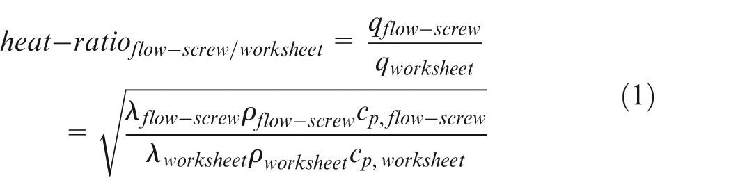
where λ is the thermal conductivity, ρ is the mass density and c_p is the specific heat of the flow screw/worksheet material.

Regarding the problem of heat transfer between the flow screw and worksheets, although the flow screw and worksheets initially contact only through surface asperities and air-filled pockets exist in the contact regions, the convection and radiation heat transfer across these pockets were neglected and pure conduction heat transfer was assumed in this work. The reasons for this assumption are as follows: (a) the temperature in the contact region is too low for significant radiation during the FS process and (b) convection currents are unlikely to form in the small and isolated interfacial pockets.

The conduction heat transfer between the contacting surfaces is defined as the product of interfacial thermal conductance and the temperature difference between the contacting surfaces. The interfacial thermal conductance is known to depend on the surface topology, contact pressure and material thermo-mechanical properties.^12,13

The surface asperities deform plastically under the high contact pressures and interfacial temperatures encountered in the course of the FS process, giving rise to high values of the interfacial thermal conductance. For this reason, temperature jumps are expected to be negligibly small, and temperature continuity is assumed across the contact interface.

Material models

The flow screws are typically made of air-hardening cold-work tool steels, such as AISI A2. The flow screw generally experiences very little elastic and practically no plastic deformation during the FS process due to high strength of these steel grades at elevated temperatures. Consequently, the flow screw is assumed to be made of a rigid material with a mass density of 7865 kg/m³, and the thermal and thermo-mechanical properties assigned are as follows: (a) thermal conductivity, k = 37.5 W/m K; (b) specific heat, c_p = 473 J/kg K and (c) linear coefficient of thermal expansion, α = 10.8 × 10⁻⁶/K.

The workpiece material employed in this analysis is AA5059-H131, which is a solid-solution strengthened and strain-hardened/stabilized Al–Mg–Mn alloy. The Johnson–Cook material model^14,15 is used to describe the behavior of this material, which is assumed to be isotropic, linear-elastic and strain-hardenable, strain rate sensitive, thermally softenable plastic.^16,17

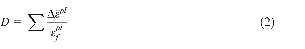
The worksheet materials displaced and plastically deformed by the rotating and piercing flow screw can also sustain damage and, concomitantly, experience a loss in stiffness and strength. To model this process, the classical Johnson–Cook progressive-damage/ductile-failure model ¹⁰ is employed. The progress of failure according to this model is defined by the following cumulative damage law

$$D=\sum \frac{\Delta {\overline{\epsilon }}^{\mathrm{pl}}}{{\overline{\epsilon }}_f^{\mathrm{pl}}}$$

(2)

where $\Delta {\overline{\epsilon }}^{\mathrm{pl}}$ is the increment in equivalent plastic strain with an increment in loading and ${\overline{\epsilon }}_f^{\mathrm{pl}}$ is the equivalent plastic failure strain at the current state of loading which is a function of the mean stress, the effective stress, the strain rate and the homologous temperature, given by

$${\overline{\epsilon }}_f^{\mathrm{pl}}=[D_3+D_4\exp (D_5\sigma *)][1+D_6\ln {\stackrel{·}{\epsilon }}_{\mathrm{pl}}][1+D_7{T}_{H0}]$$

(3)

where σ* is the mean stress normalized by the effective stress. The parameters D₃, D₄, D₅, D₆ and D₇ are all material-specific constants. Material failure (i.e. a complete loss of load-carrying capacity) is assumed to occur when the damage parameter D = 1.

Computational algorithm

During FS process simulation using a conventional Lagrangian finite element analysis, the elements generally experience a large degree of distortion, causing the analysis to become inaccurate and prone to failure, for example, Grujicic et al. ¹⁸ For this reason, the FS process is simulated using a new combined Eulerian–Lagrangian (CEL)–based finite element analysis. ¹⁹ Within this analysis, the flow screw is modeled as a Lagrangian sub-domain, the worksheets as part of an Eulerian sub-domain and the interaction between the two is modeled using an Eulerian/Lagrangian contact algorithm (presented earlier). An explicit solution algorithm implemented in ABAQUS/Explicit, ¹⁰ a general-purpose finite element solver, is employed to solve the fully coupled thermo-mechanical problem dealing with the FS process.

Typical results

In this section, an example of the prototypical FS process simulation results is presented and discussed. These results were obtained for the following set of process/material parameters: (a) worksheet material: AA5059-H131; ²⁰ (b) top worksheet thickness: 1.9 mm, bottom worksheet thickness 5.8 mm; (c) flow screw material: AISI A2 tool steel; (d) flow screw design: Boellhoff RIVTAC^®; (e) flow screw rotational speed/feed rate: (1) stage 2—5000 r/min or 20 mm/s and (2) stage 3—800 r/min or 2 mm/s and (f) flow screw axial torque/thrust force of 300 N m or 80 N in stage 4.

Spatial distribution and temporal evolution of the Eulerian/Lagrangian materials during the FS process simulation are presented in Figure 3(a)–(d). Examination of the results displayed in these figures reveals the following:

1. As the flow screw begins to penetrate the top worksheet, a collar of the top worksheet material is formed around the unthreaded part of the screw shank (Figure 3(a) and (b)).

2. Once the screw has penetrated through the top worksheet and has begun to penetrate the bottom worksheet: (a) a smaller collar containing the bottom worksheet material is formed around the unthreaded portion of the screw shank, Figure 3(b) and (b) a “through-draft” (containing the displaced top worksheet material) is formed at the back face of the bottom worksheet (Figure 3(b)).

3. As the screw begins to pass through the back surface of the bottom worksheet, a bushing is formed (Figure 3(c) and (d)).

4. Eulerian materials tend to occupy fully the portions of the Eulerian elements not occupied by the Lagrangian/screw domain. In other words, very little porosity/void can be found in the Eulerian region adjacent to the screw.

Figure 3.

Spatial distribution and temporal evolution of the Eulerian/Lagrangian materials during the FS process simulation at the relative times: (a) 0, (b) 1, (c) 2 and (d) 3.

Virtual mechanical testing of FS joints

Modeling and computational analysis

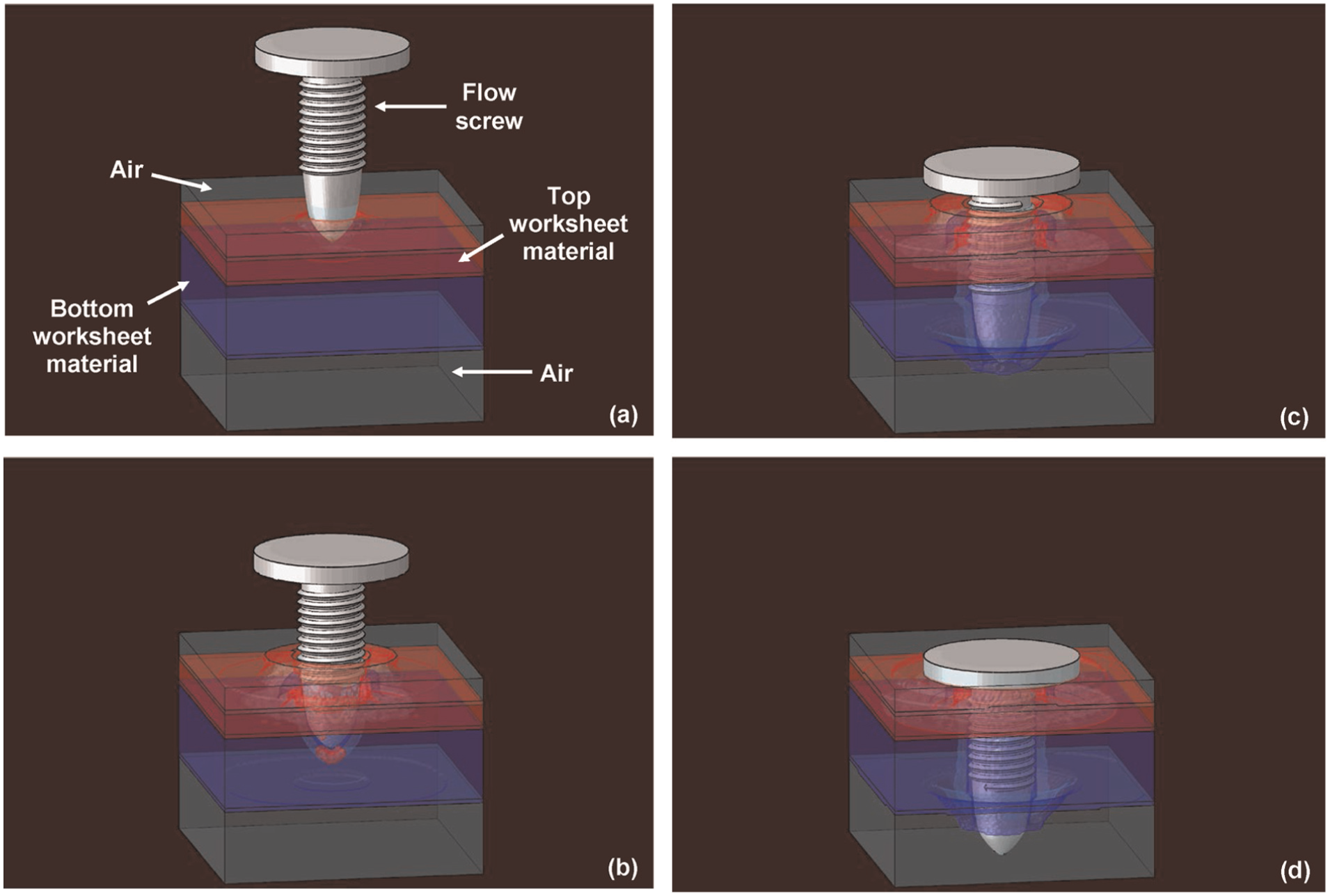
The problem analyzed in this portion of the work deals with virtual mechanical testing ²¹ of the FS joints. Four types of virtual mechanical tests are used: (a) normal-pull (also known as U-shaped tension) test, (b) shear test, (c) 45° oblique-pull test and (d) peel test. Unique details of the finite element analysis used to simulate these tests are presented in this section.

Geometrical and meshed models

Examples of the geometrical models used in this portion of the work are depicted in Figure 4(a)–(d). The four geometrical models pertain, respectively, to the cases of (a) a normal-pull test, (b) a shear test, (c) an oblique-pull test and (d) a peel test. The four test-specimen geometries differ only in the number (one or two, per worksheet), location (top/bottom, left/right) and orientation (vertical vs oblique) of the bent end sections. These end sections are used for specimen gripping during virtual testing. Geometrical boundaries for the flow screw and the upper and lower worksheets (in the vicinity of the FS joint) are obtained by mapping the Eulerian material distribution results of the finite element modeling of the FS process to a 3D Lagrangian geometrical model. The remainder of the upper and lower worksheets is reconstructed by simply assuming that their geometries/thicknesses were not affected by the FS process. The vertical and oblique end sections are obtained by bending the worksheet ends over a 4.0-mm radius rigid/immobile rod. For each of the test specimens, the direction of the applied loading is indicated, in Figure 4(a)–(d), using arrows, and the (vertical) symmetry plane is labeled.

Figure 4.

Geometrical models used in the FS joint virtual mechanical testing: (a) normal-pull, (b) shear, (c) 45° oblique-pull and (d) peel test specimens.

The newly created Lagrangian-type geometrical models for the two worksheets have been meshed using continuum four-node, first-order tetrahedron elements. The mesh in the vicinity of the FS joint has been refined to enable more accurate capture of the mechanical response of this region, since it experiences the largest deformation-field gradients. Sections of the upper and lower worksheets further away from the FS joint, including the vertical/oblique sections, are modeled using a coarser mesh. For brevity, examples of the typical mesh-size used are not shown.

Initial and boundary conditions

Since the FS process is associated with extensive plastic deformation of the two worksheets and introduces residual stresses and damage into the region surrounding the joint, the plastic strain, residual stress and damage fields obtained at the end of the FS process modeling had to be mapped onto the test specimens and used as initial conditions. This mapping procedure had to be carried out very carefully to ensure that the mapped stresses are self-equilibrating and do not cause extensive additional deformation (and rigid body motion) of the test specimens.

For the cases of the normal-pull, 45° oblique-pull and peel tests, the following boundary conditions were employed: (a) nodes on the bottom face of the lower, vertical/oblique section(s) have all their translational degrees of freedom (DOFs) constrained, as well as their rotational DOFs about the longitudinal and loading directions and (b) nodes on the top faces of the upper, vertical/oblique section(s) are subjected to a constant velocity in the loading direction. This velocity was not directly applied to the nodes associated with the subject face(s). Instead, the velocity is applied through a translator-type connector, a connector in which the only available DOF is the translation of the two nodes along the line connecting them (the line coinciding with the loading direction). The bottom node of the translator connector was joined with the subject top face(s) using a coupling kinematic constraint (a constraint that couples the DOFs of the nodes residing on the subject surface to the corresponding DOFs of a reference node, the bottom node of the translator connector in this case). The stiffness of the translator connector is then selected in such a way as to match the combined stiffness of the loading piston and the specimen gripping device. Finally, the velocity in the loading direction is applied to the upper node of the translator connector. As far as the remaining DOFs of the nodes residing on the top face(s) of the upper, vertical/oblique section(s) are concerned, they were constrained in the same way as their counterparts for the nodes residing on the bottom face(s) of the lower, vertical/oblique section(s).

For the case of the shear test, the following boundary conditions were employed: (a) nodes on the leftmost face of the lower, vertical section have all their translational DOFs constrained, as well as their rotational DOFs about the longitudinal (pulling) and the vertical directions and (b) nodes on the rightmost face of the upper, vertical section are subjected to a constant rightward velocity. Again, the velocity was not directly applied to the nodes of the subject face, but rather through the combination of a translator-type connector and a coupling kinematic constraint. As far as the remaining DOFs of the nodes residing on the rightmost face of the upper, vertical section are concerned, they were constrained in the same way as their counterparts for the nodes residing on the leftmost face of the lower, vertical section.

Typical results

Material evolution

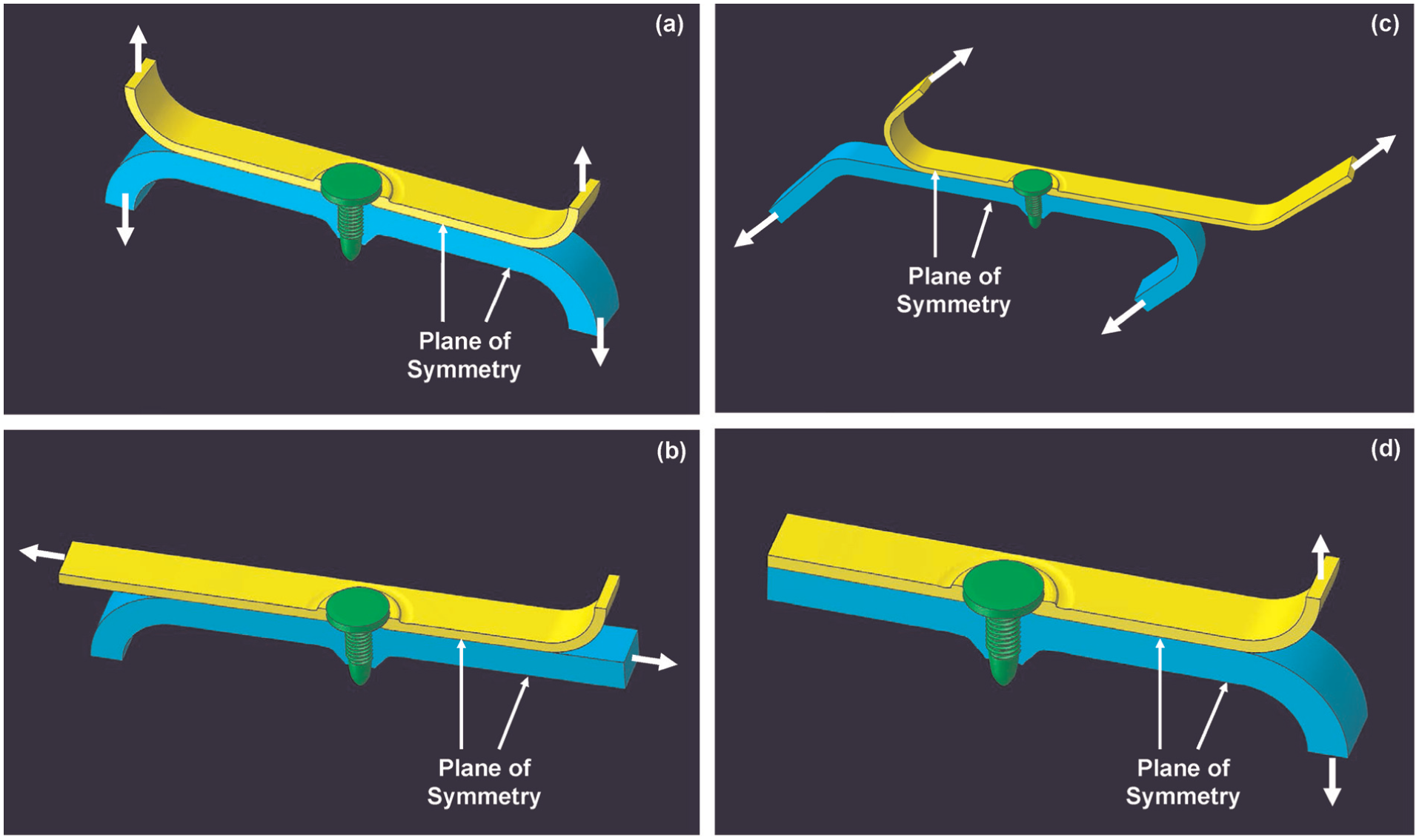
Figure 5(a)–(d) shows typical results pertaining to the spatial distribution and temporal evolution of the (rigid) flow screw, top worksheet and bottom worksheet materials during the normal-pull test. Examination of the results displayed in Figure 5(a)–(d) reveals that (a) the damage to the FS joint has been almost entirely localized within the bottom worksheet; (b) as the normal-pull test proceeds, the extent of damage in the bottom worksheet increases; (c) within the bottom worksheet, the damage is primarily localized in the region adjacent to the threaded portion of the screw and in the collar and (d) before the final loss of load-carrying capacity takes place within the FS joint, some of the damaged bottom worksheet material breaks off, forming loose chips/debris.

Figure 5.

An example of the results pertaining to the spatial distribution and temporal evolution of the flow screw, top worksheet and bottom worksheet materials during the normal-pull test at the relative times: (a) 0, (b) 1, (c) 2 and (d) 3.

For brevity, the corresponding results associated with the shear, 45° oblique-pull and peel tests are not shown. However, they will be briefly described below. In the case of the shear test, damage was localized on the loaded side of the bottom worksheet threaded region. Similarly, in the case of the oblique-pull test, damage was concentrated on the loaded side of the bottom worksheet threaded region. In the case of the peel test, the screw was rotated from its vertical position before it was pulled out from the bottom worksheet. This caused damage on one side of the bottom worksheet in the lower portion of the threaded region, and on the other side in the upper portion of the same region.

Load versus displacement

Typical load versus displacement curves obtained in this portion of the work for the normal-pull, shear, 45° oblique-pull and peel tests are depicted in Figure 6(a)–(d). Presently, there are no experimental results for AA5059-H131 FS joints which can be used for validation of the present computational procedure. However, in Holmstrøm and Sønstabø, ⁹ the experimental results are provided for AA6016-T4 alloy. These results are displayed as insets in Figure 6(a)–(d). Comparison of the present computational results with their experimental counterparts from Holmstrøm and Sønstabø, ⁹ shown in Figure 6(a)–(d), reveals that the general shapes of the corresponding force versus displacement curves are similar. The computational results displayed in Figure 6(a)–(d) will be further analyzed in the next section, where they will be compared with their counterparts obtained using the shell representation of the sheets and the connector representation of the flow screw.

Figure 6.

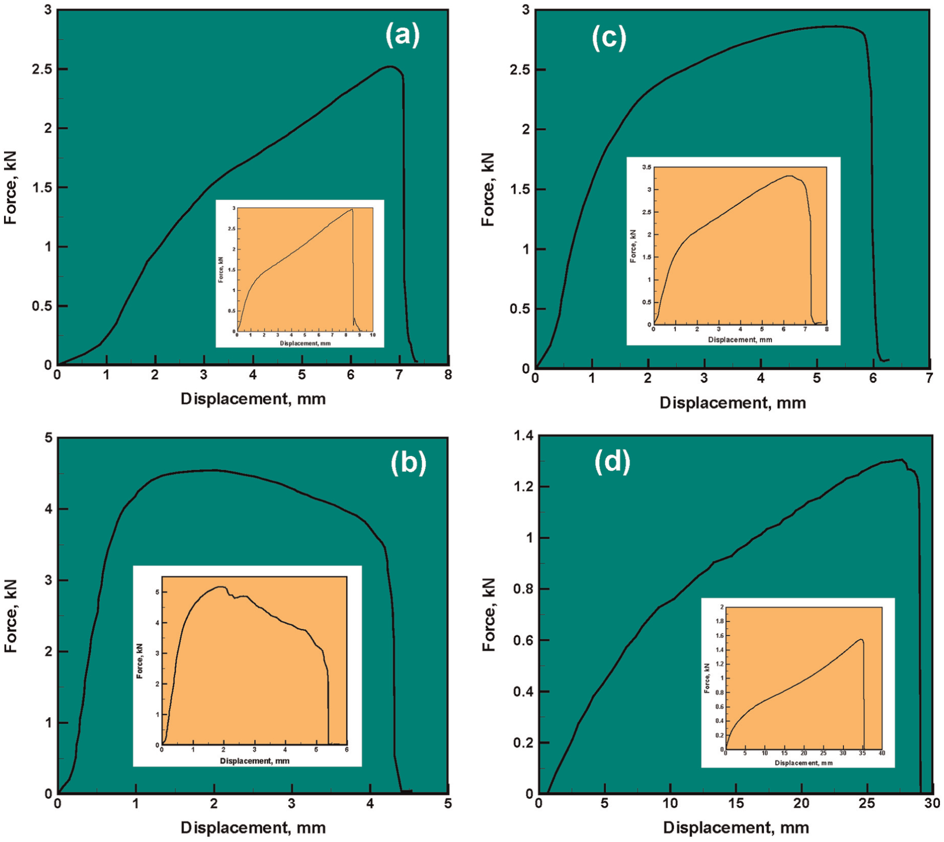
Examples of the present computational load vs. displacement results obtained during (a) normal-pull, (b) shear, (c) 45° oblique-pull and (d) peel tests of AA5059-H131 FS joint. Insets contain the corresponding experimental results for AA6016-T4 FS joint. ⁹

Construction of the FS joint connectors

Derivation of the connector constitutive relations

In whole-vehicle crash simulations, detailed 3D models of the FS joints are commonly replaced with the appropriate structural (point-to-point) connector elements. The basic force versus displacement and moment versus rotation relations characterizing elastic and plastic deformation, damage and ultimate failure of the FS joint connectors are derived and parameterized using the results of the finite element simulations like the ones discussed in the previous section (as well as the experimental results). In this section, a brief description is provided of the procedures used to derive and parameterize the governing deformation/failure relationships of the FS connectors. The constitutive relations for the FS joint connector are derived under the following conditions, assumptions and simplifications: (a) a local connector coordinate system is used, within which the connector is aligned with the x₃-direction, while directions x₁ and x₂ lie in the plane of the fastened worksheets; (b) elastic responses of the connector associated with each of the three translational and rotational DOFs are assumed to be independent/decoupled; (c) the fastened joint is assumed to be axisymmetric; (d) the elastic stiffness about the axis of symmetry of the FS connector (sixth DOF) is assumed to be fixed and controlled by the magnitude of the torque applied in the fourth stage of the FS process. In other words, the fact that the sixth-DOF elastic stiffness generally increases as the screw is tightened and decreases as the screw is loosened is not taken into account; (e) plastic behavior of the connector is described in a manner similar to the conventional metal plasticity and involves specifications of the yield potential, flow rule and the hardening/constitutive relations and (f) damage initiation and damage evolution relations are assumed to mimic those encountered in the case of ductile failure involving voids’ nucleation, growth and coalescence.

Elastic behavior

In accordance with the assumptions made above regarding the linear and decoupled character of the elastic response, as well as regarding free rotation about the connector axis (x₃), the elastic response of the FS connector is fully defined using five elastic stiffnesses E_i , i = 1–5.

Plastic behavior

The connector plastic response is defined through specification of the yield criterion, flow rule and hardening behavior. The driving force promoting plastic response of the connector is assumed to be governed by the following yield potential function

$$P={[{\left(\frac{F_N}{R_N}\right)}^{\beta }+{\left(\frac{F_S}{R_S}\right)}^{\beta }]}^{1/\beta }$$

(4)

where the equivalent normal force, $F_N$ , and equivalent shear force, $F_S$ , are, respectively, defined as

$$F_N=\left|f_3\right|+\frac{K}{r}\sqrt{m_1^2+m_2^2}$$

(5)

$$F_S=\sqrt{f_1^2+f_2^2}$$

(6)

where i = 1, 2, 3 denotes three components of a vector associated with the three coordinate axes; $f$ denotes a force; $m$ a moment; $r$ is the rivet radius and $R_N$ , $R_S$ , $\beta$ and $K$ are the connector yield potential parameters.

The onset and continuation of the plastic response are then assumed to be governed by the following yield criterion

$$\varphi =P(f_1,f_2,f_3,m_1,m_2)-F^0\left({\overline{u}}^{\mathrm{pl}}\right)\ge 0$$

(7)

where $F^0$ is the force equivalent of the yield strength, and ${\overline{u}}^{\mathrm{pl}}$ is the equivalent plastic relative motion (a quantity analogous to the equivalent plastic strain in metal plasticity).

Evolution of the plastic relative motion ${\overline{u}}^{\mathrm{pl}}={[u_1^{\mathrm{pl}},u_2^{\mathrm{pl}},u_3^{\mathrm{pl}},u_{r1}^{\mathrm{pl}},u_{r2}^{\mathrm{pl}}]}^T$ (where subscript $r$ denotes a rotational DOF, while superscript $T$ a transpose operator) is assumed to be governed by the associated/normality flow rule as

$${\stackrel{·}{u}}^{\mathrm{pl}}={\stackrel{·}{\overline{u}}}^{\mathrm{pl}}·\frac{\partial \varphi }{\partial f}$$

(8)

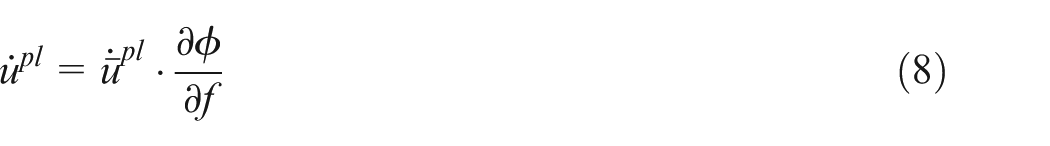
where a raised dot denotes a time derivative, and the generalized force vector is defined as $f={[f_1,f_2,f_3,m_1,m_2]}^T$ . The equivalent plastic relative motion rate and the equivalent plastic relative motion are then defined as

$${\stackrel{·}{\overline{u}}}^{\mathrm{pl}}=\sqrt{\frac{{\left({\stackrel{·}{u}}^{\mathrm{pl}}\right)}^T·\left({\stackrel{·}{u}}^{\mathrm{pl}}\right)}{(\frac{\partial \varphi }{\partial f^T}·\frac{\partial \varphi }{\partial f})}}$$

(9)

$${\overline{u}}^{\mathrm{pl}}=\underset{0}{\overset{t}{\int }}{\stackrel{·}{\overline{u}}}^{\mathrm{pl}}\mathrm{dt}$$

(10)

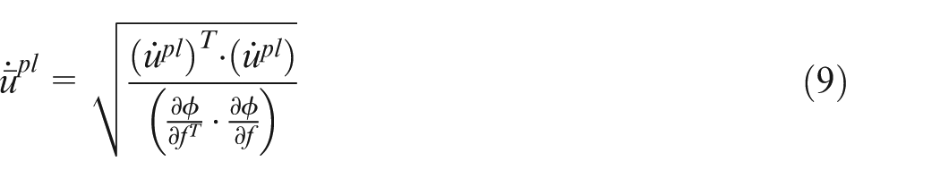
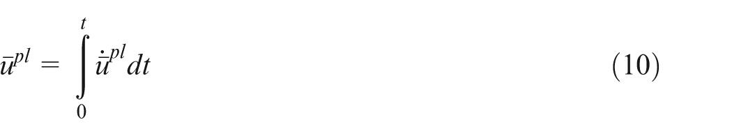
Equation (10) yields ${\overline{u}}^{\mathrm{pl}}=R_S·u_1^{\mathrm{pl}}$ for the case of pure shear in direction 1 and ${\overline{u}}^{\mathrm{pl}}=R_N·u_3^{\mathrm{pl}}$ for the case of pure tension in the axial direction x₃.

As plastic deformation proceeds, the connector is assumed to experience isotropic strain-hardening. Consequently, $F^0$ in equation (7) controls the size of the (fixed-shape) yield surface. As plastic deformation proceeds, ${\overline{u}}^{\mathrm{pl}}$ and, thus, $F^0$ increases, causing an expansion of the yield surface. Thus, hardening behavior is fully described by the $F^0$ versus ${\overline{u}}^{\mathrm{pl}}$ functional relationship (to be determined using a calibration procedure).

Damage initiation and evolution

As plastic deformation continues, the equivalent plastic relative motion crosses a critical value beyond which the connector continuously incurs internal damage. Both the critical value of ${\overline{u}}^{\mathrm{pl}}$ and the rate of damage evolution/accumulation are generally found to be functions of the connector loading angle (i.e. loading mode mixity). The loading mode mixity ${\Psi }_m$ is defined here as

$${\Psi }_m=\frac{2}{\pi }·{\tan }^{-1}\left(\frac{F_N}{F_S}\right)$$

(11)

Clearly, ${\Psi }_m=0.0$ for the case of pure shear, and ${\Psi }_m=1.0$ for the case of pure normal loading. Damage initiation is then fully defined by a ${\overline{u}}_{\mathrm{DI}}^{\mathrm{pl}}$ versus ${\Psi }_m$ functional relationship, where subscript DI denotes damage initiation.

As internal damage accumulates within the connector, its strength is assumed to decrease linearly with an increase in ${\overline{u}}^{\mathrm{pl}}$ . At ${\overline{u}}^{\mathrm{pl}}={\overline{u}}_f^{\mathrm{pl}}$ , connector strength becomes 0, causing it to fail. Under this simplifying assumption, damage evolution is fully defined by a $({\overline{u}}_f^{\mathrm{pl}}-{\overline{u}}_{\mathrm{DI}}^{\mathrm{pl}})$ versus ${\Psi }_m$ relation. This functional relationship, as well as the ${\overline{u}}_{\mathrm{DI}}^{\mathrm{pl}}$ versus ${\Psi }_m$ functional relationship, have to be determined using a calibration procedure. Due to their intrinsic mathematical complexity, both these functional relationships are often defined using a piecewise linear representation.

Parameter identification and calibration

Before the parameters pertaining to the elastic, plastic and damage/failure response of the connector are defined, it was recognized that the contribution of the bending moments $m_1$ and $m_2$ to the overall loading is small (and, hence, can be neglected) in the cases of normal-pull, pure shear and 45° oblique-pull loading. However, the bending moments generally make a substantial contribution in the case of peel tests. Since the contribution of the bending moments to the overall loading is proportional to the parameter $K$ in equation (5), normal-pull, pure shear and 45° oblique-pull virtual testing results are first used to determine the remaining parameters and functional relations defining the connector constitutive behavior. Then, the peel test results are used to determine $K$ .

Elastic behavior

Using the elastic portions of the force versus displacement results obtained under normal-pull, pure shear and 45° oblique-pull loading conditions, and employing a curve-fitting procedure, the first three elastic stiffness constants are determined as follows: E₁ = E₂ = 3.15 MN/m and E₃ = 3.69 MN/m. Following prior work of Weyer et al., ²² E₄ and E₅ are assumed to be infinite (a rigid-elastic approximation). E₆ has already been defined as a fixed torque-controlled quantity.

Plastic behavior

To fully define the plastic response of the FS connector, $R_N$ , $R_S$ , $\beta$ and the $F^0$ versus ${\overline{u}}^{\mathrm{pl}}$ relation must be defined. To determine $R_S$ and $R_N$ , the following procedure was employed:

1. It is first established that the initial level of the connector strength, $F_0^0$ , is independent of the mode of loading.

2. At the peak load under normal-pull, pure shear and 45° oblique-pull loading, the connector acquires the same (maximum) level of its strength, $F_{max}^0$ .

3. By combining equations (4) and (7), the following relation: $F_I^0=F_J^I/R_J,I=0,max,J=N,S$ is obtained. Using this relation, the plastic portions of the force versus displacement curves (up to the onset of damage), and a curve-fitting procedure, $R_N=21.1$ and $R_S=32.3$ , are obtained.

The parameter $\beta$ is obtained by curve-fitting different 45° oblique-pull force versus displacement results in the plastic region (up to the onset of failure) to the relation obtained by combining equations (4) and (7). This procedure yielded $\beta =1.57$ .

The $F^0$ versus ${\overline{u}}^{\mathrm{pl}}$ (strain-hardening) relationship is obtained by (1) extrapolating the elastic response of the connector into the elastic/plastic region and (2) estimating the plastic relative displacement (as a difference between the total and the elastic relative displacements) at different levels of $F^0$ . This procedure yielded the functional relationship $F^0$ versus ${\overline{u}}^{\mathrm{pl}}$ depicted in Figure 7.

Figure 7.

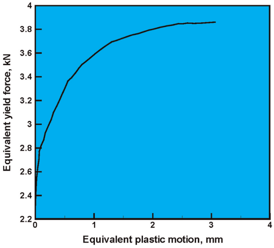
Equivalent yield force versus equivalent plastic displacement hardening behavior of the FS connector.

Damage initiation and evolution

To define the ${\overline{u}}_{\mathrm{DI}}^{\mathrm{pl}}$ versus ${\Psi }_m$ functional relationship, it was first assumed that damage initiates at the point of maximum load. Then the sought-after functional relationship is obtained by simply determining the equivalent plastic relative displacement associated with the corresponding peak loading for different tests, each corresponding to a different value of ${\Psi }_m$ . An example of the ${\overline{u}}_{\mathrm{DI}}^{\mathrm{pl}}$ versus ${\Psi }_m$ functional relationship obtained is depicted in Figure 8(a).

Figure 8.

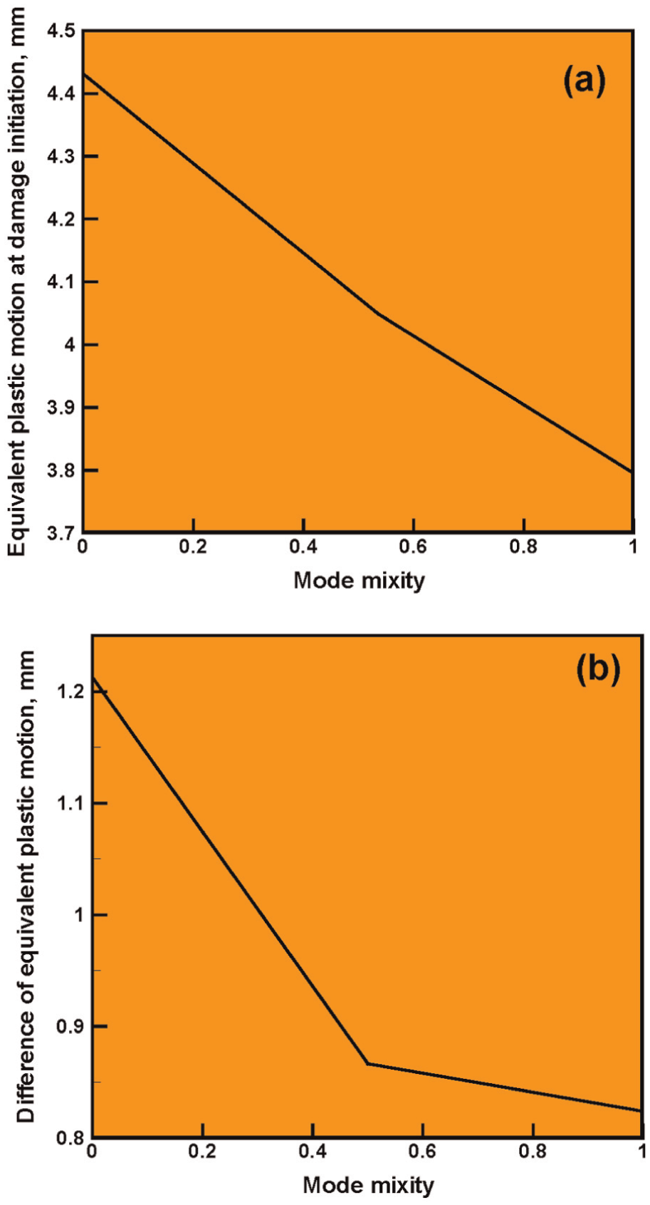
Effect of mode mixity on the (a) equivalent plastic motion at damage initiation and (b) the additional post-damage-initiation equivalent plastic motion at the point of failure in an FS connector.

To calibrate the $({\overline{u}}_f^{\mathrm{pl}}-{\overline{u}}_{\mathrm{DI}}^{\mathrm{pl}})$ versus ${\Psi }_m$ functional relationship, it is first recognized that in the post-damage-initiation portion of the load versus displacement curves, the mixity ratio changes during loading (except for the cases of pure normal and pure shear loading). Taking this into account, combining all the post-damage-initiation force versus displacement data, and utilizing a linear regression analysis, the piecewise linear form of the $({\overline{u}}_f^{\mathrm{pl}}-{\overline{u}}_{\mathrm{DI}}^{\mathrm{pl}})$ versus ${\Psi }_m$ functional relationship depicted in Figure 8(b) is obtained.

Parameter $K$ in equation (5)

To determine the last unknown parameter $K$ , an optimization procedure was employed in conjunction with the finite element simulations (for the peel test) as described in the next section. Within these simulations, riveted sheets are modeled as shell structures while the FS joint is modeled as the connector constructed and parameterized in this section. Within the optimization procedure, parameter $K$ was used as a single design variable while the extent of agreement between the peel test load versus displacement results obtained in section “Virtual mechanical testing of FS joints” and in the present section was defined as the objective function. This optimization procedure yielded $K=0.51$ .

Validation procedure

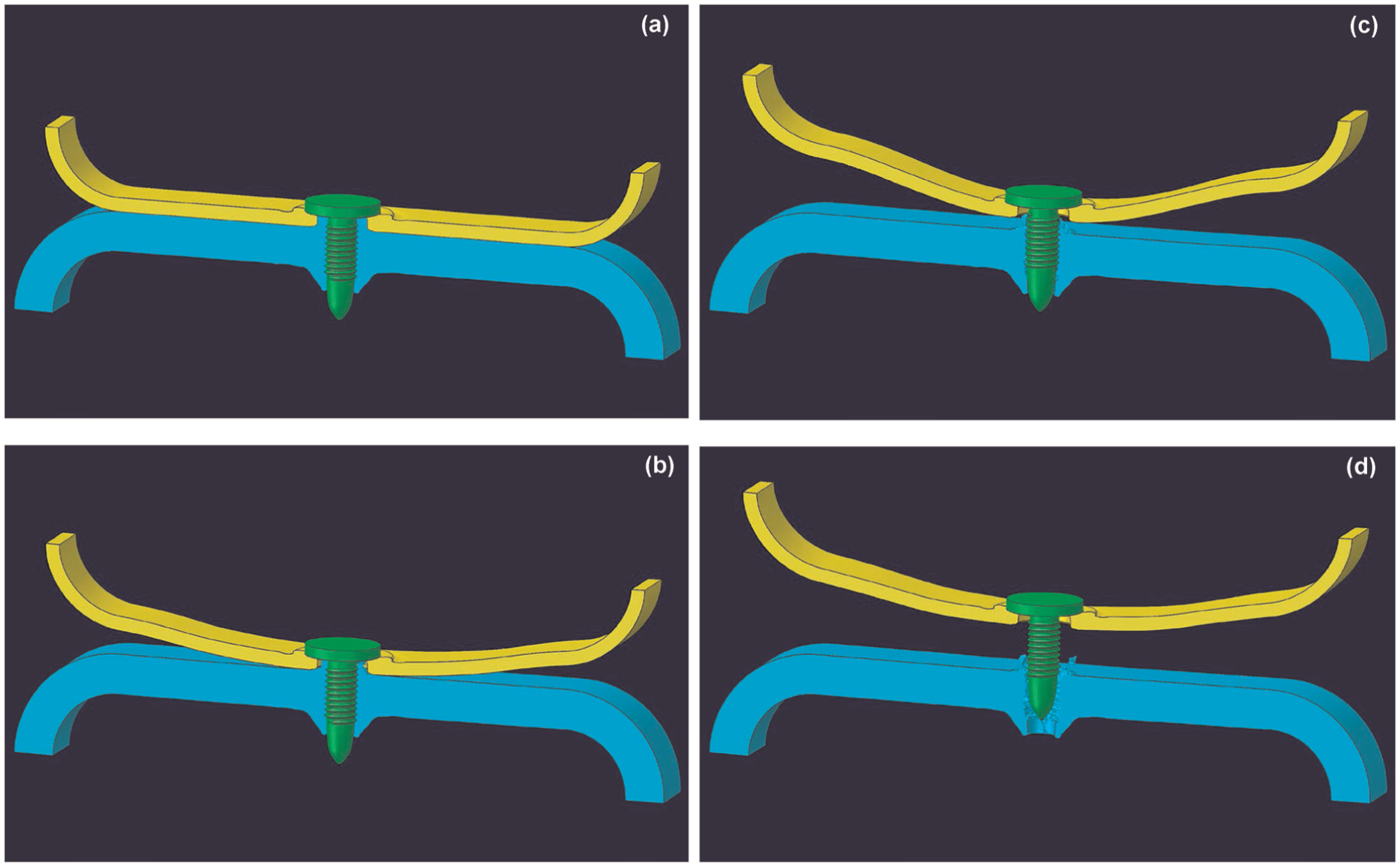
As mentioned earlier, FS joint connectors are typically used in whole-vehicle simulations in which fastened sheet-metal structures are represented as shells. To validate the derived and parameterized constitutive relations for the FS connector (described above), virtual (normal-pull, shear, 45° oblique-pull and peel) tests of fastened shell-type specimens are carried out. In these simulations, the fastened connections between the sheets are represented using the just-derived FS connectors. An example of the finite element mesh used (for the case of pure-normal/pull loading) is depicted in Figure 9. The domain of influence^23–26 is indicated in this figure, as well as the connector.

Figure 9.

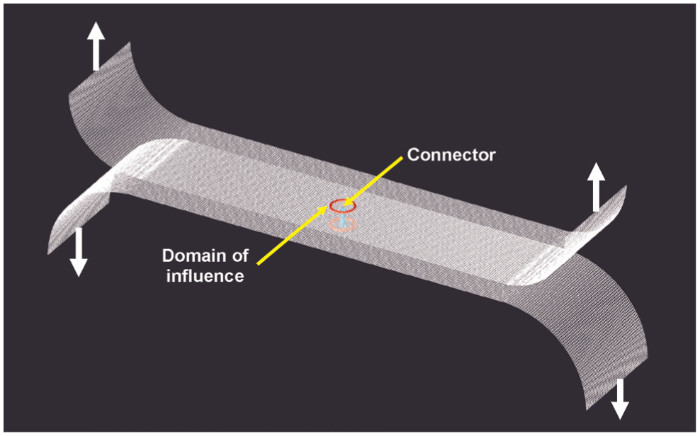
Finite element mesh used (for the case of pure-normal/pull loading) of the FS joint modeled as an assembly of two shell-type worksheets and a connector-type screw. See text for explanation of the term “domain of influence.”

Temporal evolution of the material within the two shells (fastened by an FS-joint connector), during the normal-pull test, is depicted in Figure 10(a)–(d). A comparison of these results with their counterparts in Figure 5(a)–(d) reveals that (a) the overall evolutions of the worksheet materials, represented either as 3D continuum structures or 3D shells, are comparable and (b) before the final failure of the joint, the bottom worksheet begins to experience damage in the region surrounding the joint.

Figure 10.

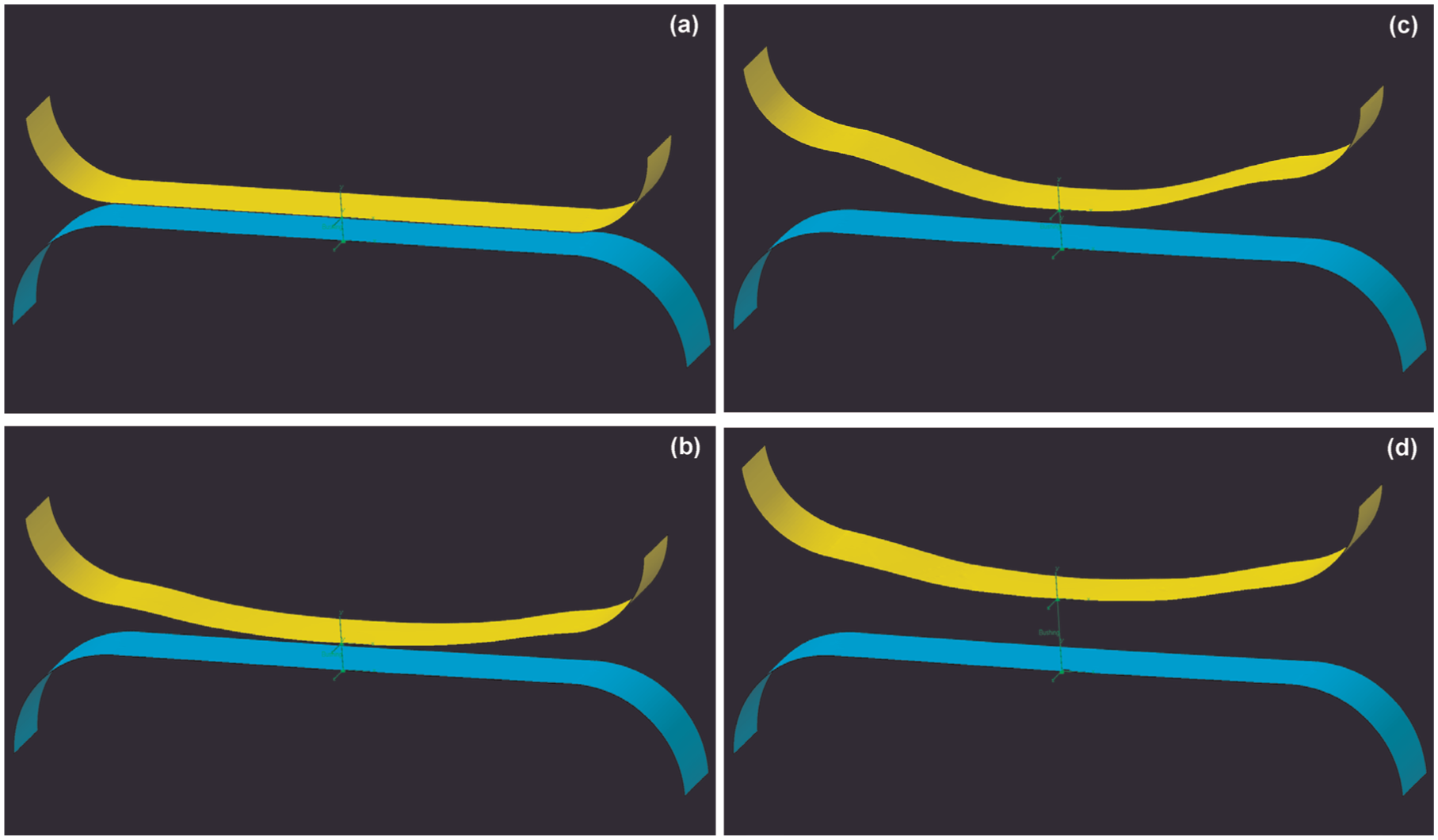
Temporal evolution of the material within the two shells (fastened by FS joint connector) during the normal-pull test at the relative times: (a) 0, (b) 1, (c) 2 and (d) 3.

Figure 11(a)–(d) displays the load versus displacement results for the normal-pull, shear, 45° oblique-pull and peel tests obtained in this portion of the work. These results are labeled as “FS-Joint Connector.” For comparison, the corresponding results obtained in section “Virtual mechanical testing of FS joints” are also shown in these figures. These results are labeled as “3-D FS Joint.”

Figure 11.

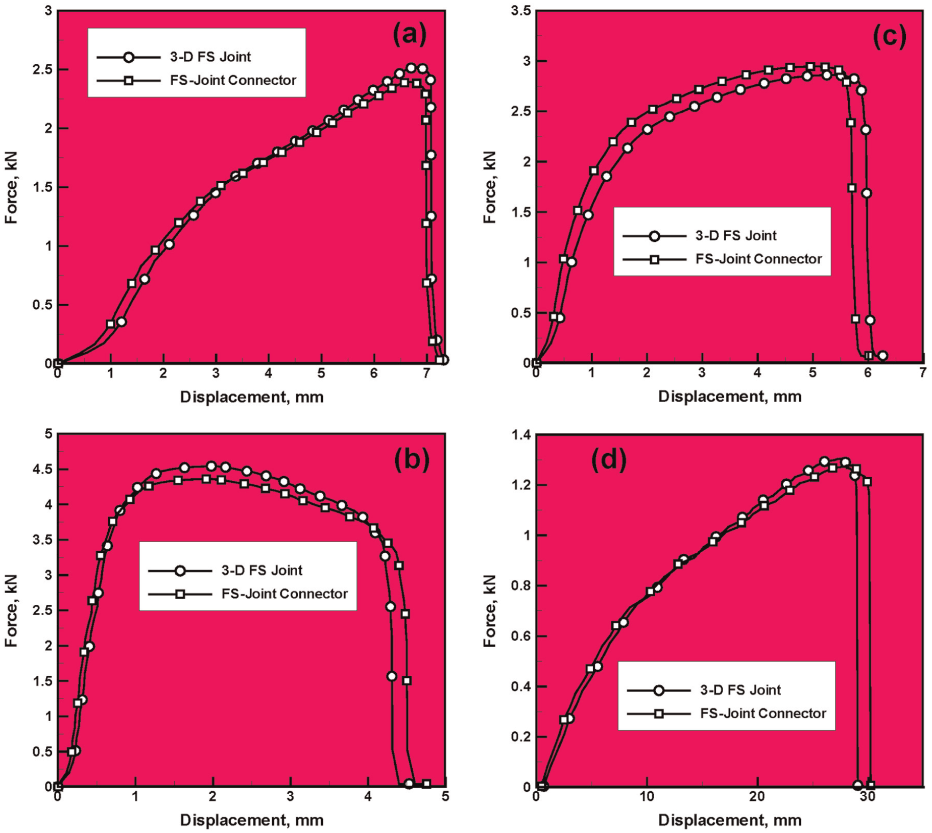
A comparison of the load vs displacement results obtained in the virtual testing of solid (three-dimensional) FS joints and shell sections fastened by FS joint connectors: (a) normal-pull, (b) shear, (c) 45° oblique-pull and (d) peel tests.

Examination of the results displayed in Figure 11(a)–(d) reveals that the overall level of agreement between the two (FS-Joint Connector and 3-D FS Joint) sets of results for each of the four tests is satisfactory, relative to the joint strength (as quantified by the maximum force), joint ductility (as quantified by the maximum displacement before a complete loss of the load-carrying capacity) and the overall toughness (as quantified by the area under the load vs displacement curve). This finding suggests that the FS connectors can reasonably well account for the mechanical response of the very detailed 3D continuum FS joints.

Summary and conclusion

Based on the results obtained in this work, the following main summary remarks and conclusions can be drawn:

1. A three-step computational procedure is developed to establish dependence of the mechanical properties of the flow screw (FS) mechanical joints on the FS process parameters: (a) flow screw design and material, (b) worksheet-metal thicknesses and materials and (c) history of the flow screw rotational speed, feed rate, axial torque and thrust force.

2. This procedure involves finite element modeling and simulations of the FS process and virtual testing of the resulting FS joints under different types of loading such as normal-pull, shear, 45° oblique-pull and peeling.

3. The results of the virtual mechanical testing are used to construct and parameterize FS joint point-to-point line-connector elements. These elements are needed in large-scale simulations of whole-vehicle crash in the vehicle-body manufacturing process (e.g. car-body electro-coat paint-baking process).

4. Virtual testing of the shell components fastened using the joint connectors validated the ability of these line elements to realistically account for the strength, ductility and toughness of the 3D FS joints.