Sage Journals: Discover world-class research

Abstract

An analytical and finite element investigation of the effect of different cryogenic cooling nozzle configurations on temperature and residual stress in a model friction stir weld is presented. A new configuration adopting a distributed cooling approach is proposed based on an analytical cooling model. Finite element models are implemented to verify the effect of distributed cooling on welding temperature and longitudinal residual stress. The results presented indicate that new active cooling methods can improve mitigation of welding-induced residual stress.

Keywords

Distributed cooling active cooling residual stress friction stir welding finite element analysis

Introduction

Friction stir welding (FSW), invented by TWI in 1990,^1–5 is a solid-state welding process in which heat from a rotating tool softens the material along a join line in the workpiece, enabling mechanical mixing of the material along the weld. The process is known for its capability to join metals that are difficult to weld using conventional fusion welding techniques, such as high-strength aluminium alloys.^6–10 Figure 1 shows a schematic of the FSW butt welding process. Compared to conventional fusion welding, FSW usually results in lower residual distortion due to the relatively low thermal input to the workpiece. However, the process induces residual stress that could influence the mechanical performance^11–13 and the mechanical–chemical performance^14,15 of the welds.

Figure 1.

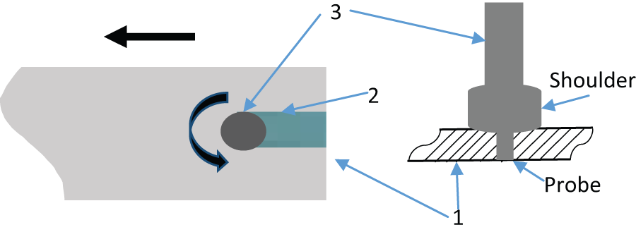
Schematic representation of FSW process.

To investigate the factors that influence residual stress, researchers have investigated various materials and process parameters using numerical methods such as the finite element (FE) method. These studies have mainly focused on residual stress caused by unbalanced heat progress during welding. Using a simplified two-dimensional (2D) model incorporating the pin effect to material flow patterns, Zhang et al.¹⁶ found that longitudinal residual stress of the weld was symmetric to the welding line, with an M-shaped transverse profile. In addition, the maximum longitudinal residual stress was found to vary with welding velocity. Khandkar et al.¹⁷ investigated thermal residual stress in sequentially coupled three-dimensional (3D) simulation, considering aluminium alloys and steel. The properties of all three materials were treated as temperature dependent. The predicted results showed good agreement with data reported by other researchers^18,19 and indicated that longitudinal tensile stress was the main component of residual stress in all three cases. More complex and realistic material models, heat source models and boundary conditions have been studied by other workers.^20–26 These investigations indicated that thermal-induced stress contributed the majority to the residual stress with the largest component in the longitudinal direction.

Use of active cooling to control residual stress in both conventional fusion welding and FSW has been widely reported. The effect of a cooling source was investigated through FE modelling and experimental validation by Van der Aa²⁷ for aluminium alloy and steel, although there is a risk of martensite formation and consequent cracking for carbon steels due to the rapid cooling. The results indicated that cooling sources trailing the welding torque can reduce residual stress, as well as buckling distortion induced by fusion welding. Furthermore, it was observed that increasing cooling power above 6000 W m⁻² K did not have a significant effect on further reducing residual stress. Staron et al.²⁸ applied liquid CO₂ cooling media to friction stir–welded Al sheets by experiment and found tensile residual stresses in the weld zone were reduced significantly and it was even possible to generate compressive residual stress, which is considered to be able to improve fatigue life for components. Richards et al.²⁹ modelled the progress of active cooling applied to FSW using liquid CO₂ and also identified that there is a cooling power limit, above which little reduction in residual stress occurs. They also investigated a two-nozzle strategy aimed at further reduction in longitudinal residual stress but without success. This was attributed to the near-seam areas getting colder and yield strength becoming higher, making it difficult to generate more tensile plastic strain.

This article presents an analytical and numerical investigation of the effect of cooling nozzle configuration and a new distributed cooling method proposed. As the welding temperature plays an important role in FSW,³⁰ the effect of high cooling power on welding temperature is investigated when applied close to the heating source. The resulting longitudinal residual stress was studied in particular, as this has been shown to be a significant stress component.^31,32

Nozzle configurations and analysis

According to investigations in Richards et al.,²⁹ active cooling can generate tensile plastic strain to compensate compressive plastic strain incurred during welding. It is therefore only effective when the nozzle is placed trailing the welding tool. A common configuration for active cooling is shown in Figure 2(a). The left circle indicates that the cooling nozzle used is a cylinder perpendicularly placed to workpiece top surface. The cooling nozzle’s diameter Dc is usually not smaller than that of the tool diameter Dt. The cooling rate within the nozzle is usually considered to be uniform. For convenience of investigation, the cooling nozzle in this article is rectangular, as shown in Figure 2(b) (referred as non-distributed cooling), and its width of cooling area Wca and length of cooling area Lca are 10 and 20 mm, respectively.

Figure 2.

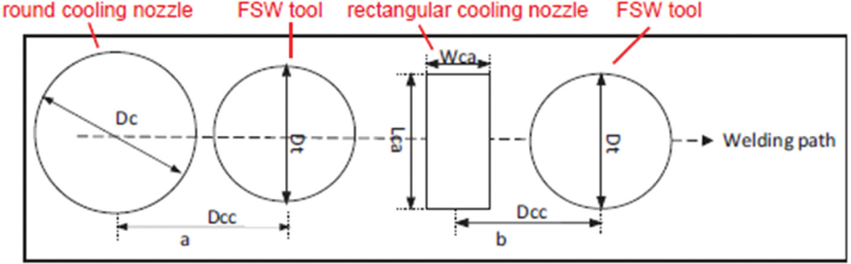
Schematics for non-optimized cooling nozzle.

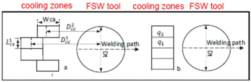
Another nozzle configuration (referred as distributed cooling) is presented in Figure 3. The cooling nozzle is divided evenly into four zones, as shown in Figure 3(a), each with adjustable distance centre-to-centre $D_{cc}^{i}$ (for i = 1 and 2; i = 3 or 4 is not shown due to symmetry). Theoretically, the cooling rate $q_{i}$ (i = 1, 2) of the zones can be different, as shown in Figure 3(b), but physically precise control of its distribution might be difficult in practice and this approach is not considered here.

Figure 3.

Schematics for distributed cooling.

Welding temperature

Provided the cooling nozzle is close enough to the heat source, applying active cooling will decrease welding temperature of the material under the welding tool. To simplify the analysis presented in this section, 2D planar heat transfer is assumed and the material properties related to heat transfer calculations are temperature independent.

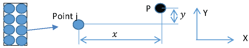
The cooling area is equally discretized into n points (or lines through the thickness), as shown in Figure 4. The temperature increment of point P during the time increment from 0 to $t$ due to one of the n cooling points, point j, can be expressed as equation (1),³³ which is derived from Laplace’s equation

Figure 4.

Schematic for welding temperature analysis.

T = \frac{Q}{4 π α cpht} \exp (\frac{- r^{2}}{4 α t})

(1)

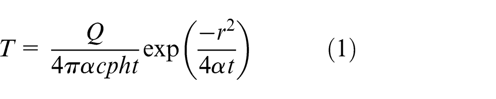
where T represents the temperature after time t; Q is the instantaneous energy input (negative); h is the thickness of plate; $α$ , $c$ and $p$ are the constant material property parameters thermal diffusivity, specific heat and density, respectively; $r$ is the distance between point P and point j and $t$ is the time duration since the line heating source applied.

Based on temperature cumulative law, the temperature induced by a non-distributed cooling source and a distributed cooling source can be expressed as equations (2) and (3), respectively

\begin{matrix} T_{cool}^{nc} = \sum_{j = 1}^{n} \int_{0}^{t_{0}} \frac{qdt}{4 π cp α h (t_{0} - t)} \\ \exp (\frac{- [{(x_{j}^{nc} - vt)}^{2} + y_{j}^{nc 2}]}{4 α (t_{0} - t)}) \end{matrix}

(2)

\begin{matrix} T_{cool}^{dc} = \sum_{j = 1}^{n} \int_{0}^{t_{0}} \frac{qdt}{4 π cp α h (t_{0} - t)} \\ \exp (\frac{- [{(x_{j}^{dc} - vt)}^{2} + y_{j}^{dc 2}]}{4 α (t_{0} - t)}) \end{matrix}

(3)

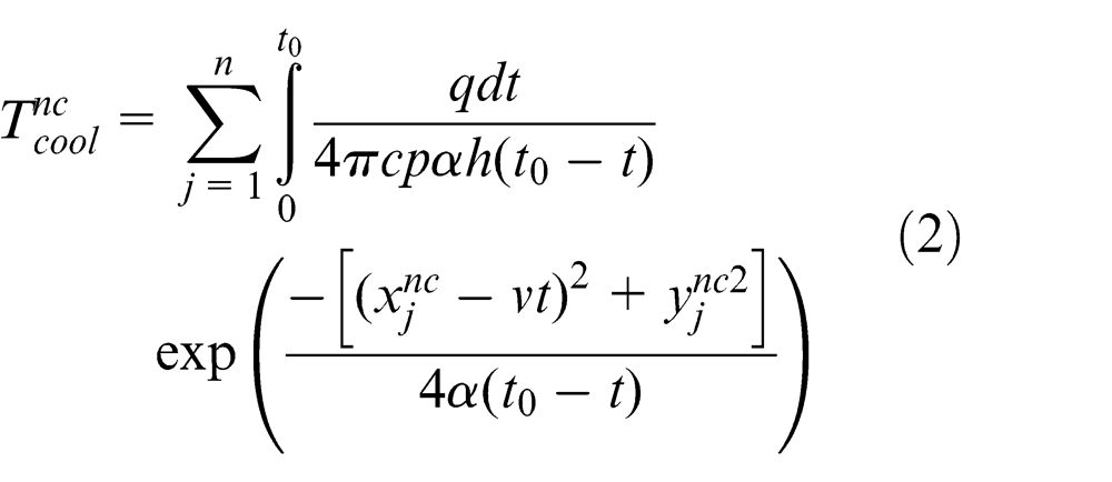
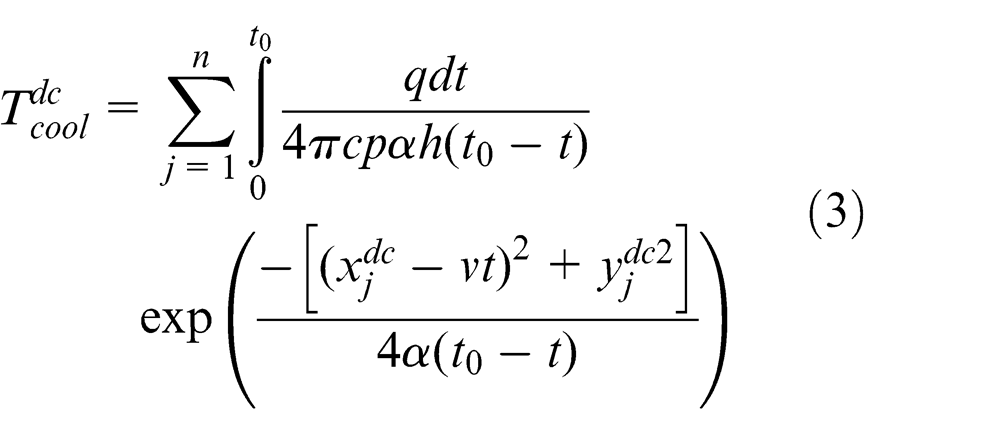
where n is the total amount of discrete points; $T_{cool}^{nc}$ and $T_{cool}^{dc}$ are the temperature increment of point P from time 0 to $t_{0}$ in the non-distributed and distributed cooling models, respectively; $q$ is the cooling rate of point j in the non-distributed and distributed cooling models; $x_{j}^{nc}$ , $y_{j}^{nc}$ and $x_{j}^{dc}$ , $y_{j}^{dc}$ are the X and Y coordinate distances between point j and point P in the non-distributed cooling model and distributed cooling model and v is the welding velocity. When t = t ₀, $x_{j}^{nc} - vt > 0$ .

$x_{j}^{dc} > x_{j}^{nc}$ and $y_{j}^{dc} = y_{j}^{nc}$ when point C belongs to zone 1;

$x_{j}^{dc} = x_{j}^{nc}$ and $y_{j}^{dc} = y_{j}^{nc}$ when point C belongs to zone 2.

Thus, $T_{cool}^{dc} > T_{cool}^{nc}$ , indicating that the welding temperature in the distributed cooling model is higher than that of the non-distributed cooling.

Temperature gradient

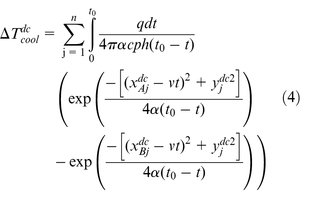
The temperature gradients between points A and B, as shown in Figure 5, for the distributed cooling and non-distributed cooling are expressed by equations (4) and (5), respectively (material properties are assumed constant)

\begin{matrix} Δ T_{cool}^{dc} = \sum_{j = 1}^{n} \int_{0}^{t_{0}} \frac{qdt}{4 π α cph (t_{0} - t)} \\ (\exp (\frac{- [{(x_{Aj}^{dc} - vt)}^{2} + y_{j}^{dc 2}]}{4 α (t_{0} - t)}) \\ - \exp (\frac{- [{(x_{Bj}^{dc} - vt)}^{2} + y_{j}^{dc 2}]}{4 α (t_{0} - t)})) \end{matrix}

(4)

Δ T_{c o o l}^{n c} = \sum_{j = 1}^{n} \int_{0}^{t_{0}} \frac{q d t}{4 π α c p h (t_{0} - t)} (\exp (\frac{- [{(x_{A j}^{n c} - v t)}^{2} + y_{j}^{d c 2}]}{4 α (t_{0} - t)}) - \exp (\frac{- [{(x_{B j}^{n c} - v t)}^{2} + y_{j}^{d c 2}]}{4 α (t_{0} - t)}))

(5)

Figure 5.

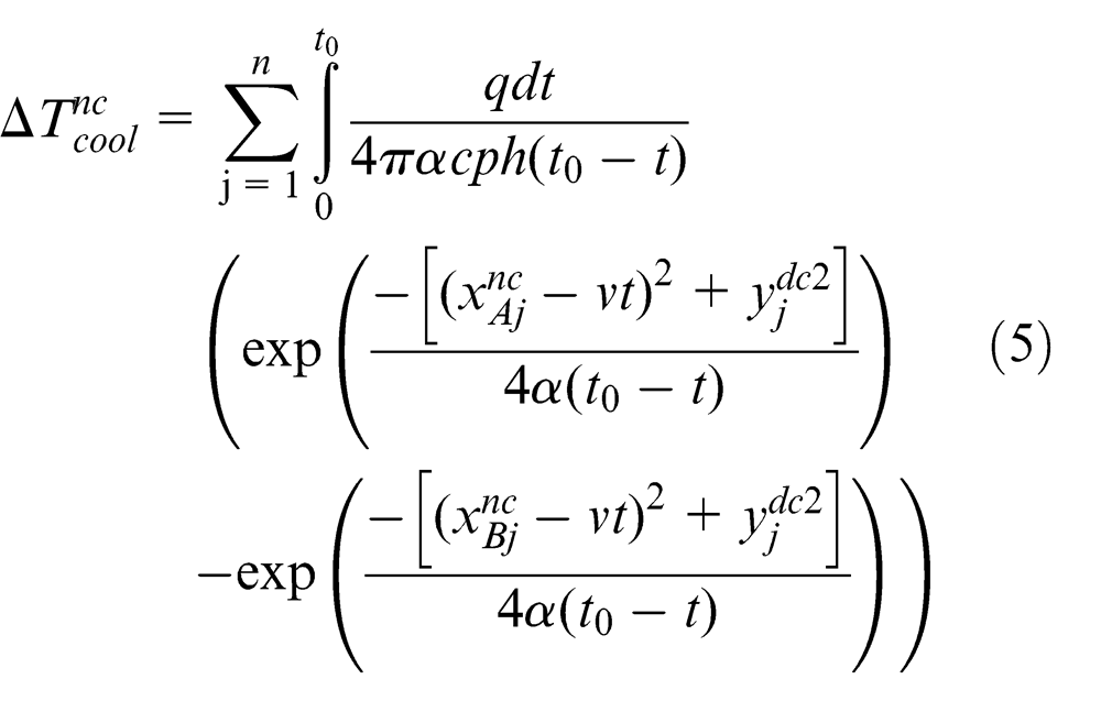
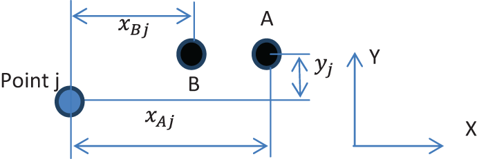
Schematics of temperature gradient analysis.

where $Δ T_{cool}^{dc}$ is the temperature difference between point A and point B in the distributed cooling and $Δ T_{cool}^{nc}$ is the temperature difference between point A and point B in the non-distributed cooling.

For point j in zone 2

Δ T_{cool}^{dc} = Δ T_{cool}^{nc}

(5)

For point j in zone 1

Δ T_{cool}^{dc} < Δ T_{cool}^{nc}

(5)

Therefore, the temperature gradient for the material under the welding tool could be reduced by distributed cooling. The lower temperature gradient indicates lower local temperature-induced tensile stress after the tool has passed.

Temperature-dependent material properties

The mechanical properties of the metals such as aluminium alloys and steels are temperature dependent and they become softer at higher temperature. Figure 6 shows a temperature–yield strength curve for aluminium alloy AA2024. The temperature dependence of the strength influences the effect of active cooling. To generate tensile plastic strain, it is better to place the active cooling power as close as possible to the welding tool, where the material is hot and temperature gradient is high. However, as the temperature drops quickly between the tool and cooling source, the material quickly becomes more difficult to yield.

Figure 6.

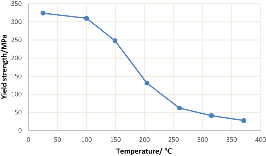
Temperature-dependent yield strength for aluminium alloy 2024.

Although the longitudinal temperature gradient in distributed cooling will be smaller than that of the non-distributed cooling, the local temperature itself is higher, giving a possibility of lower longitudinal residual stress.

FE analysis modelling

The analyses presented in sections ‘Welding temperature’ and ‘Temperature gradient’ are simplified and provide a qualitative description of the effect of distributed cooling. To achieve a quantitative assessment of the effect of the distributed cooling arrangement, ABAQUS Standard-based thermal–mechanical coupled FE models were used. The FE models include the thermal effect of the welding tool but do not include mechanical effects such as material stirring and local forces. Three cooling arrangements are considered: no active cooling, non-distributed cooling and distributed cooling.

In the ABAQUS-based models, the main heat source is the friction between the welding tool and the material, which is modelled as a heat flux in the FE model. It moves synchronously with the welding tool and is applied as a user-defined load implemented by user subroutine DFLUX (ABAQUS user subroutine to apply user-defined heat flux).³⁴ DFLUX is programmed in FORTRAN and it defines the heat flux distribution and variation with time. It is called at each step increment and heat flux inputs for the elements are updated.

The passed-in parameters in DFLUX include step time, total time, coordinates, flux type, surface name and so on. The step time and total time can be used to calculate the reference position based on welding velocity. The coordinates are the current coordinates of the current point and are represented by a vector. In case that multiple types of heat flux are involved, the heat flux type is identified as either body flux or surface flux. The surface name helps to identify different surface heat fluxes in different surfaces if necessary.

The basic implementation of DFLUX to define the moving heat source in the present investigation is shown in Figure 7. When the ABAQUS main program needs the heat flux value at an integration point, it calls DFLUX. First, it calculates the current position of heat source centre based on the current step time and constant welding velocity. Then the distance between the integration point and the heat source centre is judged if within the radius of the welding tool’s shoulder. The heat flux value of the integration point is determined by the total power input and the distance and is returned to the ABAQUS main program.

Figure 7.

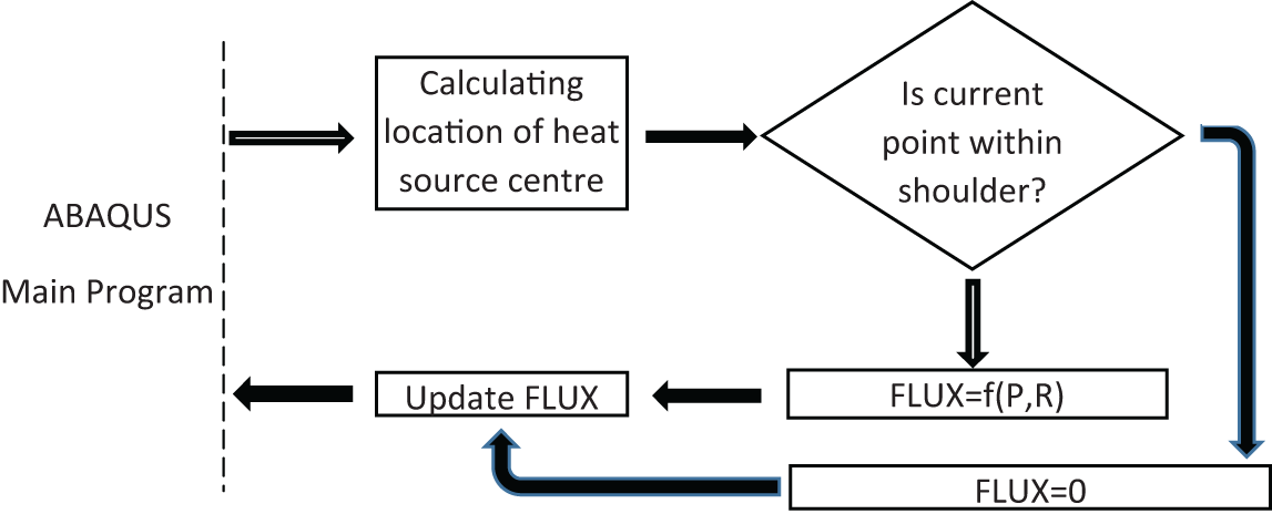
Work flow of user subroutine DFLUX.

The active cooling and heat loss between the workpiece and support plate are defined as user-defined interaction and implemented in a user subroutine FILM (ABAQUS user subroutine to apply user-defined film coefficient).³⁴ The passed-in parameters of FILM include step time, total time, coordinates, flux type, surface name and so on. The step time and total time are used to calculate the tool position based on the welding velocity. The coordinates are those of the current point and are represented by a vector. The flux type defines the film condition type (when multiple types of non-uniform film conditions are involved). The surface name relates different surface film conditions to different surfaces. The parameters to be defined in the FILM include the film coefficient and sink temperature for the current point and film coefficient rate with respect to time.

Figure 8 illustrates the implementation of the FILM for the distributed active cooling. First, the requested film coefficient defines whether there is active cooling or natural heat loss, based on the surface name of the current integration point and its coordinates. If it is for active cooling, the current coordinates of the welding tool centre are determined, based on step time and welding velocity. Then the location of the current integration point is identified as either inside or outside the cooling area. Finally, the film coefficient value for active cooling is calculated.

Figure 8.

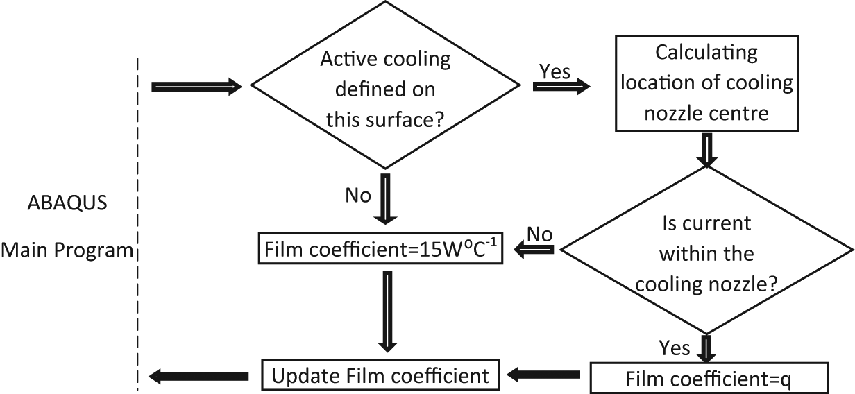
Work flow of user subroutine FILM.

The models can be divided into two separated steps, namely, the welding step and natural cooling step. In the welding step, the heating source and active cooling (if applicable) are loaded.

Geometry

The model workpiece comprises two plates with dimensions of 50 mm × 150 mm × 3 mm. Only half is modelled due to symmetric geometry, boundary conditions and loads, as shown in Figure 9. The welding tool moves along the X+ axis.

Figure 9.

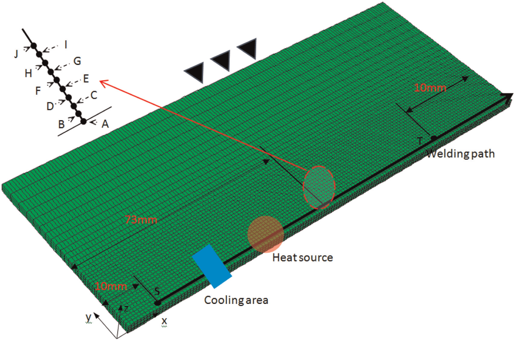
Finite element model for friction stir welding.

Material properties

The material investigated is AA2024, which has the following properties:

Thermal conductivity = 121 W m⁻¹ °C⁻¹;

Thermal expansion coefficient = 2.268 E−5 °C⁻¹;

Density = 2780 kg m⁻³;

Young’s modulus = 73.1 GPa;

Poisson’s ratio = 0.33.

The temperature-dependent yield strength properties³⁵ are listed in Table 1.

Table 1.

Yield strength variation with temperature for AA2024.³⁵

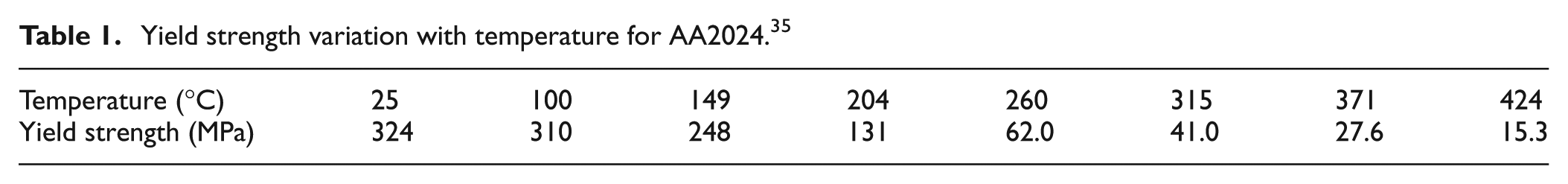
Temperature (°C)	25	100	149	204	260	315	371	424
Yield strength (MPa)	324	310	248	131	62.0	41.0	27.6	15.3

The temperature-dependent values for Young’s modulus from Brammer and Percival³⁶ and thermal expansion coefficient from ASM International³⁷ are also examined to assess the sensitivity of residual stress to temperature dependence of these properties.

Boundary conditions and loads

Physically, the workpiece is in contact with a rigid backing plate. As representing this contact interaction using a contact algorithm is computationally expensive, this is simplified to a zero Z-direction (vertical) constraint applied to the bottom face of the workpiece in the mechanical model. Heat loss from the other faces to air through radiation and convection is incorporated in the film condition, where the ambient temperature is constant 25 °C and film coefficient is 15 W m⁻² °C⁻¹. A symmetry boundary condition is applied in the Z–X plane.

In the welding step, the heat loss rate for the bottom face area directly under the welding tool should be larger than other areas because of its Z-axis force.⁵ Here, the assumed film coefficient in this area is 500 W m⁻² °C⁻¹, while for other areas it is 200 W m⁻² °C⁻¹. The total heat input power is programmed in DFLUX as 700 W surface heat flux in a circular area of radius 10 mm. The welding speed is 5 mm s⁻¹.

In the non-distributed cooling models and distributed cooling models, the cooling source moves at the same velocity as the tool. The Y-direction of one side of the plate is constrained, as shown in Figure 9. In the natural cooling step, the heat input and active cooling are removed, as well as the Y-direction constraint on the side.

The welding starts 10 mm away to one side and ends 10 mm away to the other side, as shown in Figure 9. In the natural cooling step, all loads and clamps are released.

Mesh

The element type used in the model is C3D8RT. The mesh is graduated such that the elements increase in size as the location moves from the welding path. A mesh dependence study was performed to determine a suitable mesh size near the welding path. As shown in Figure 10, changing mesh size from 1 to 2 mm³ does not significantly change the temperature curve. The model contains 16,200 elements and 22,348 nodes.

Figure 10.

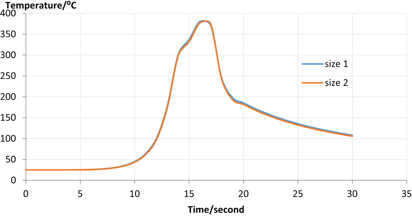
Mesh independence investigation.

Output and solver control

To balance calculation accuracy/convergence and computational cost, the time increment size in both welding step and natural cooling step is automatically controlled. The maximum increment is limited to 0.1 s in the welding step and 1.0 s in the natural cooling step. The non-linear geometry feature is turned on in the solver. The results are output every second in the welding step and every 20 s in natural cooling step.

Results and Discussion

No active cooling model

In the model with no active cooling, the temperature profile in the moving coordinate system attached to the welding tool is similar to an oval, as shown in Figure 11. The temperature field for weld time greater than 14 s is seen to be quasi-static, with the maximum welding temperature increment in the region of 2 °C s⁻¹. The reference points identified in Figure 9 achieve their maximum temperature at this moment. Their longitudinal residual stress distribution in the transverse direction is representative of most workpiece area.

Figure 11.

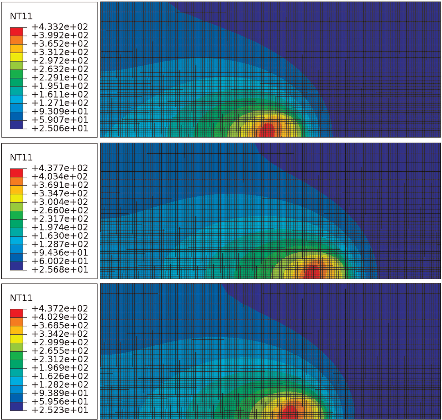
Temperature field for the no active cooling model at different weld times.

The maximum longitudinal residual stress (also referred to as MAX S11) calculated for the no active cooling model is 176.5 MPa. The longitudinal residual stress of the weld is tensile except in the welding start and end sections, and a high value is observed near the tool edge, as shown in Figure 12.

Figure 12.

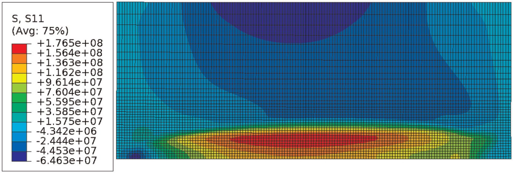
Longitudinal residual stress for the no active cooling model.

Figure 13 shows the longitudinal residual stress distribution along the reference line. The peak value is located 8 mm from the welding path (where the tool shoulder radius is 10 mm).

Figure 13.

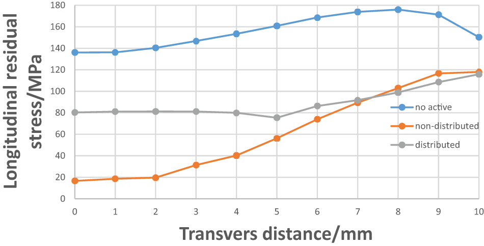
Longitudinal residual stress distribution of the no active cooling, non-distributed cooling and distributed cooling.

Non-distributed cooling model

The temperature distribution in the model with active cooling at time t = 14 s is shown in Figure 14. The distribution close to the cooling nozzle is significantly different to the distribution for no active cooling shown in Figure 11. The welding temperature under the tool is also reduced.

Figure 14.

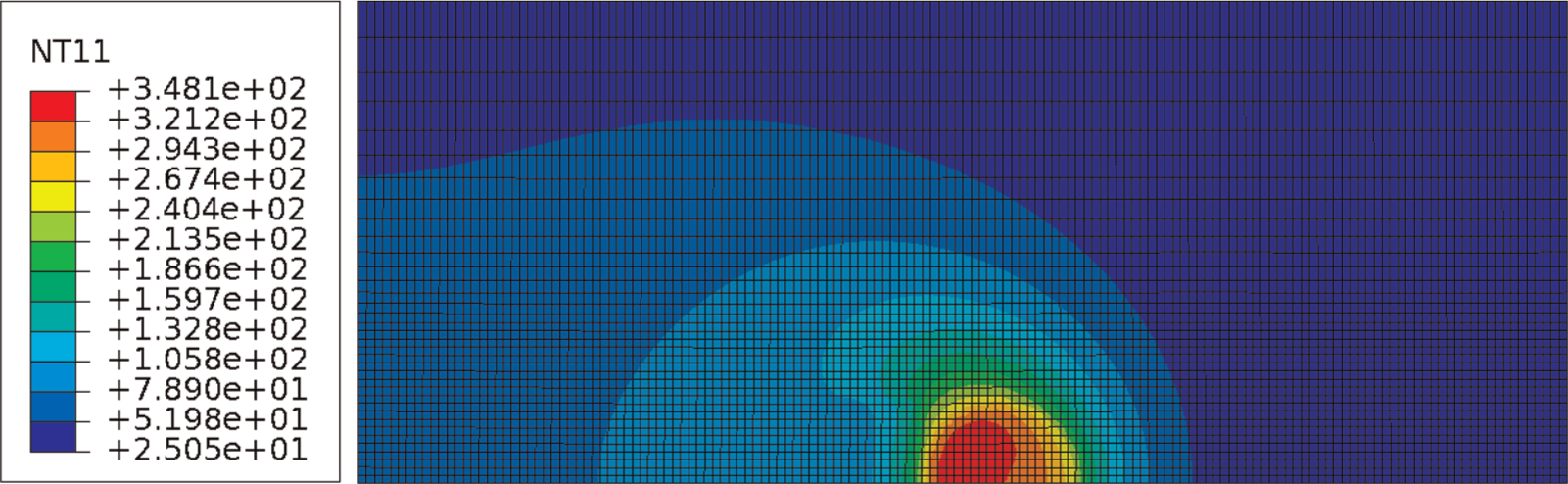
Temperature field for non-distributed cooling with Dcc = 15 mm and cooling rate = 1.6 E4 W m⁻² ° C⁻¹.

Active cooling also lowers the longitudinal residual stress. In case of Dcc = 15 mm and cooling rate = 1.6 E4 W m⁻² °C⁻¹, which is the maximum cooling rate achieved in Richards et al.,²⁹ the maximum longitudinal residual stress is 122.8 MPa, 53.7 MPa smaller than that of the no active cooling model. In addition, the longitudinal residual stress distribution along transversal direction is different, as shown in Figure 13. The disparity between the tool centre and near the edge is increased: on reference line it is 101 MPa, compared to 40 MPa in the no active cooling model.

The welding temperature drops dramatically when Dcc is decreased in Figure 15, although the longitudinal residual stress also gets lower. When Dcc = 15 mm, the welding temperature at weld time t = 14 s drops from original 433.2 °C to 348.1 °C. These findings agree well with Richards et al.²⁹

Figure 15.

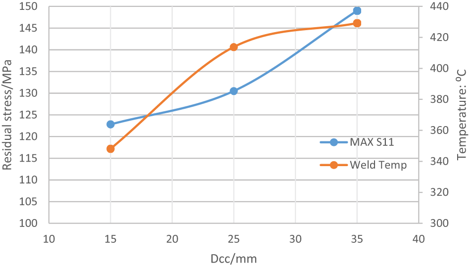
Longitudinal residual stress and welding temperature variation with Dcc for non-distributed cooling.

Distributed cooling model

Two distributed cooling arrangements are considered. In the first arrangement, Zone 1 (defined in Figure 3) is moved a further 2 mm away from the tool centre. In the second arrangement, it is moved another 2 mm.

The temperature field for distributed cooling, shown in Figure 16 for time 14 s, differs from that found for non-distributed cooling. First, the temperature contour under the cooling nozzle is almost rectangular for non-distributed cooling, as seen in Figure 14, while in distributed cooling this area becomes smaller and is not rectangular. Second, the welding temperature is increased. These changes in response are related to the adjusted cooling areas with greater centre-to-centre distances. Consequently, maximum S11 drops from 122.8 to 118.8 MPa.

Figure 16.

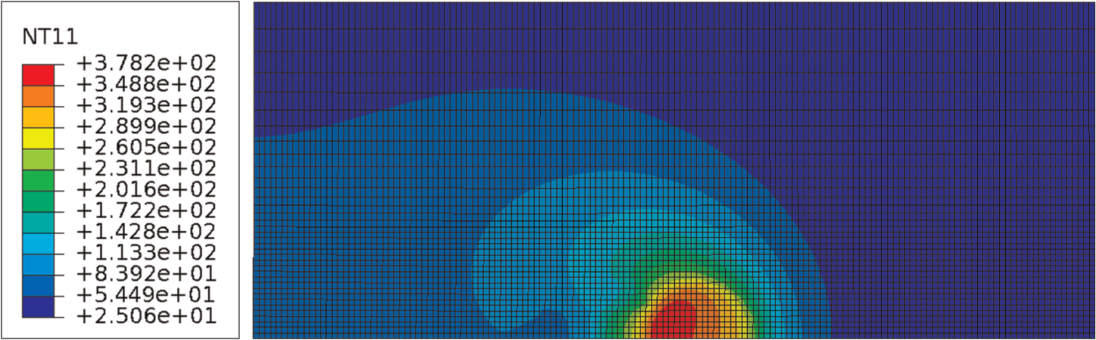
Temperature field for distributed cooling: $D_{cc}^{1} = 19 mm, D_{cc}^{2} = 15 mm$ , rate = 1.6 E4 W m⁻²°C⁻¹.

The temperature of the material under the welding tool is significantly increased in the distributed cooling models compared to the non-distributed cooling, as shown in Figure 17 at weld time t = 14 s, where Temp-dis1 identifies the first arrangement and Temp-dis2 the second. In addition, the temperature gradient is decreased, as shown in Figure 17. Here, the temperature gradient is quantified by temperature difference between two 5-mm spaced nodes (near the reference line) in the longitudinal direction.

Figure 17.

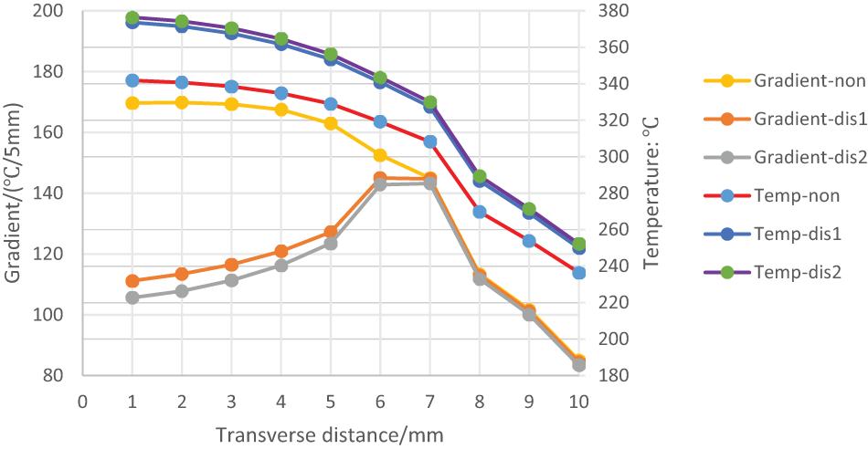
Temperature and temperature gradient compared between distributed and non-distributed cooling.

In Figure 13, the longitudinal residual stress near the welding path is increased, compared to the non-distributed cooling, while for the material near the tool edge it is slightly decreased. Although the temperature is higher at the tool centre, as shown in Figure 17, the temperature gradient is significantly decreased in distributed cooling, indicating lower tensile plastic strain will be generated after the tool has passed. For the material near the tool edge, the temperature gradient is almost the same but the temperature is increased in distributed cooling. These findings support the simplified analysis of the welding temperature and temperature gradient presented in section ‘Nozzle configurations and analysis’.

Conclusion

This article compares the temperature, temperature gradient and longitudinal residual stress for FSW processes including a non-distributed cooling model and two distributed cooling models. The main findings of the investigation are as follows:

The simplified analytical and FE models considered in the investigation indicate that distributed cooling may result in higher welding temperature than conventional cooling. In practice, this response would be influenced by factors such as the actual input heat flux, the material flow introduced by the rotating tool, the real heat conductivity, the actual cooling rate of the cooling nozzle and the convection rates.

Distributed cooling changes the temperature gradient distribution in FSW. The temperature gradient near the welding path is significantly affected by distributed cooling, while for regions away from the welding path, it is almost unaffected.

The results presented indicate that distributed cooling arrangements such as those considered could lead to improved mitigation of FSW residual stress compared to a conventional cooling arrangement of the same cooling power. The possibility of achieving both higher welding temperature and lower residual stress through distributed cooling is identified in the numerical models, indicating that the welding temperature plays an import role in reducing residual stress.

Experimental investigation of the results from the analytical and numerical models is required to validate the findings of the investigation and will be undertaken in future work.

Footnotes

Appendix 1 Declaration of conflicting interests

The authors declare that there is no conflict of interest.

Funding

This research received no specific grant from any funding agency in the public, commercial or not-for-profit sectors.

References

Mishra

. Friction stir welding and processing. Mat Sci Eng R 2005; 50: 1–78.

Cam

Mistikoglu

. Recent developments in friction stir welding of Al-alloys. J Mater Eng Perform 2014; 23: 1936–1953.

Cam

. Friction stir welded structural materials: beyond Al-alloys. Int Mater Rev 2011; 56: 1–48.

Nanda

DebRoy

Bhadeshia

HKDH

. Recent advances in friction-stir welding – process, weldment structure and properties. Prog Mater Sci 2008; 53: 980–1023.

Threadgill

Leonard

Shercliff

. Friction stir welding of aluminium alloys. Int Mater Rev 2009; 54: 49–93.

Cam

Kocak

. Progress in joining of advanced materials. Part 2: joining of metal matrix composites and joining of other advanced materials. Sci Technol Weld Joi 1998; 3: 159–175.

Ipekoglu

Erim

Cam

. Investigation into the influence of post-weld heat treatment on the friction stir welded AA6061 Al-alloy plates with different temper conditions. Metall Mater Trans A 2014; 45: 864–877.

Ipekoglu

Erim

Cam

. Effects of temper condition and post weld heat treatment on the microstructure and mechanical properties of friction stir butt-welded AA7075 Al alloy plates. Int J Adv Manuf Tech 2014; 70: 201–213.

Ipekoglu

Kiral

Cam

. Investigation of the effect of temper condition on the friction-stir weldability of Aa7075 Al-alloy plates. Mater Technol 2012; 46: 627–632.

10.

Ipekoglu

Erim

Kiral

. Investigation into the effect of temper condition on friction stir weldability of AA6061 Al-alloy plates. Kovove Mater 2013; 51: 155–163.

11.

Bussu

Irving

. The role of residual stress and heat affected zone properties on fatigue crack propagation in friction stir welded 2024-T351 aluminium joints. Int J Fatigue 2003; 25: 77–88.

12.

Altenkirch

Steuwer

Withers

. Residual stress engineering in friction stir welds by roller tensioning. Sci Technol Weld Joi 2009; 14: 185–192.

13.

Richards

Prangnell

Williams

. Global mechanical tensioning for the management of residual stresses in welds. Mat Sci Eng A: Struct 2008; 489: 351–362.

14.

Lin

Chen

. Possibility of inducing compressive residual stresses in welded joints of SS400 steels. J Mater Sci Technol 2001; 17: 661–663.

15.

Chen

Fricke

Krohn

. Experimental study of inducing compressive stress by anti-welding heating treatment in a thin plate weldment with variant temperatures. J Mater Sci Technol 2002; 18: 151–154.

16.

Zhang

Chen

. The finite element simulation of the friction stir welding process. Mat Sci Eng A: Struct 2005; 403: 340–348.

17.

Khandkar

MZH

Khan

Reynolds

. Predicting residual thermal stresses in friction stir welded metals. J Mater Process Tech 2006; 174: 195–203.

18.

Reynolds

Tang

Gnaupel-Herold

. Structure, properties, and residual stress of 304L stainless steel friction stir welds. Scripta Mater 2003; 48: 1289–1294.

19.

Sutton

Reynolds

Wang

. A study of residual stresses and microstructure in 2024-T3 aluminum friction stir butt welds. J Eng Mater: T ASME 2002; 124: 215–221.

20.

Chen

Kovacevic

. Finite element modeling of friction stir welding – thermal and thermomechanical analysis. Int J Mach Tool Manu 2003; 43: 1319–1326.

21.

Soundararajan

Zekovic

Kovacevic

. Thermo-mechanical model with adaptive boundary conditions for friction stir welding of Al 6061. Int J Mach Tool Manu 2005; 45: 1577–1587.

22.

Bastier

Maitournam

Roger

. Modelling of the residual state of friction stir welded plates. J Mater Process Tech 2008; 200: 25–37.

23.

Buffa

Fratini

Pasta

. On the thermo-mechanical loads and the resultant residual stresses in friction stir processing operations. CIRP Ann: Manuf Techn 2008; 57: 287–290.

24.

Fratini

Macaluso

Pasta

. Residual stresses and FCP prediction in FSW through a continuous FE model. J Mater Process Tech 2009; 209: 5465–5474.

25.

Buffa

Ducato

Fratini

. Numerical procedure for residual stresses prediction in friction stir welding. Finite Elem Anal Des 2011; 47: 470–476.

26.

Liu

Zhu

. Analysis of residual stresses in thick aluminum friction stir welded butt joints. Mater Design 2011; 32: 2000–2005.

27.

Van der Aa

. Local cooling during welding: prediction and control of residual stresses and buckling distortion. PhD Thesis, Delft University of Technology, Delft, 2007.

28.

Staron

Kocak

Williams

. Residual stress in friction stir-welded Al sheets. Physica B 2004; 350: E491–E493.

29.

Richards

Prangnell

Withers

. Efficacy of active cooling for controlling residual stresses in friction stir welds. Sci Technol Weld Joi 2010; 15: 156–165.

30.

Gadakh Vijay

Adepu

. Friction stir welding window for AA6061-T6 aluminium alloy. Proc IMechE, Part B: J Engineering Manufacture 2014; 9: 1172–1181.

31.

Grujicic

Arakere

. Fully coupled thermomechanical finite element analysis of material evolution during friction-stir welding of AA5083. Proc IMechE, Part B: J Engineering Manufacture 2010; 4: 609–625.

32.

Zhang

. Numerical investigations of size effects on residual states of friction stir weld. Proc IMechE, Part B: J Engineering Manufacture 2014; 4: 572–581.

33.

Zhang

. Heat transfer for welding. Beijing, China: China Machine Press 1987, pp.21–24.

34.

Dassault Systémes. ABAQUS Scripting Reference Manual V6.10. Pawtucket, USA: Dassault Systémes, 2010.

35.

Shi

. Residual stresses simulation for friction stir welded joint. Sci Technol Weld Joi 2007; 12: 664–670.

36.

Brammer

Percival

. Elevated-temperature elastic moduli of 2024 aluminum obtained by a laser-pulse technique. Exp Mech 1970; 10: 245–250.

37.

ASM International. ASM metals handbook, vol. 2. Materials Park, OH: ASM International, 1990.

A new distributed cooling method for mitigating residual stress in friction stir welding

Abstract

Keywords

Introduction

Nozzle configurations and analysis

Welding temperature

Temperature gradient

Temperature-dependent material properties

FE analysis modelling

Geometry

Material properties

Boundary conditions and loads

Mesh

Output and solver control

Results and Discussion

No active cooling model

Non-distributed cooling model

Distributed cooling model

Conclusion

Footnotes

Appendix 1

Declaration of conflicting interests

Funding

References