Modeling the cutting edge geometry of scalpel blades

Abstract

Scalpel blades are commonly used in surgery to perform invasive medical procedures, yet there has been limited research on the geometry that makes up these cutting instruments. The goal of this article is to define scalpel blade geometry and examine the cutting forces and deflection between commonly used scalpel blades and phantom gel. The following study develops a generalized geometric model that describes the cutting edge geometry in terms of normal rake and inclination angle of any continuously differentiable scalpel cutting edge surface. The parameter of scalpel-tissue contact area is also examined. The geometry of commonly used scalpel blades (10, 11, 12, and 15) is compared to each other and their cutting force through phantom gel measured. It was found that blade 10 displayed the lowest average total steady-state cutting force of 0.52 N followed by blade 15, 11, and 12 with a cutting force of 1.17 N (125% higher than blade 10). Blade 10 also displayed the lowest normalized cutting force of 0.16 N/mm followed by blades 15, 12, and 11 with a force of 0.19 N/mm (17% higher than blade 10).

Introduction

Scalpel blades are commonly used handheld instruments designed to cut tissue effectively to perform various invasive surgical procedures. These procedures include those that end with the suffix “ectomy” which means “to cut.” Common examples of this would be lumpectomy (removal of cancerous breast tissue) and prostatectomy (removal of the prostate). These are cutting processes where soft tissue is the work material and the scalpel blade acts as the tool. The goals of all these procedures are to cut tissue accurately and to minimize trauma to the patient. In order to reach these goals, sharp-edged cutting tools apply cutting forces to the tissue to fracture the bonds that hold cells in the tissue together.

Scalpels used in medicine are designated with a blade number which allows for the identification of the cutting edge shape. Figure 1 displays common industry scalpels which are used in this study. Varying the scalpel blade cutting direction allows for the use of three basic incision methods: press cutting, slide cutting, and scrape cutting, as shown in Figure 2. Utilizing these methods, tissue can be accurately removed for a wide variety of invasive surgical procedures.

Figure 1.

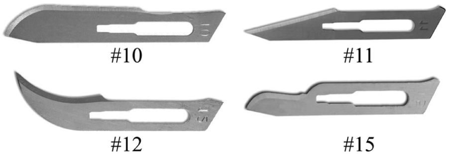
Commonly used scalpel blades.

Figure 2.

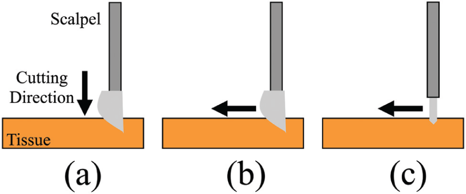
Tissue cutting techniques of (a) press cutting, (b) slide cutting, and (c) scrape cutting.

A better understanding of scalpel blade geometries can lead to improved geometry designs that can reduce the cutting forces necessary to mechanically fracture tissue. Large cutting forces generated during tissue cutting limit the design of instruments used in minimally invasive surgery (MIS). There is a continual drive in MIS procedures to reduce the number and size of the abdominal incisions using smaller instruments to reduce pain, shorten length of stay in hospital, allow for faster return to activity, and create better cosmetic outcomes. ¹ However, these small instruments must be made large enough to withstand the high tissue cutting forces they experience in operation. More effective cutting edge design can reduce the tissue cutting force and allow for the development of smaller MIS instruments.

Standardized geometric information about scalpel cutting edges will allow for scalpels to be effectively described and compared. Scalpels come in a wide variety of shapes and sizes, yet there is no research about scalpel cutting geometry, the topic of this article. Much of the work currently performed on tissue cutting instruments have examined the topics of intraoperative blood loss, operative time, operative cost, and post-operative healing time of various tissue cutting instruments including scalpels, harmonic scalpels, and electrocautery devices.^2–4 Blade tissue cutting force and modeling of forces,^5–8 as well as tissue cutting mechanics and the response of tissue under applied force,^9,10 have been previously studied. Cutting edge geometry has been a well-studied topic in traditional metal cutting to accurately identify tool cutting edges.^9,11,12 Recently, both curved and flat plane needle tip cutting edge geometries have been characterized in terms of rake, α, inclination, λ, and contact length, η.^13–15 This study standardizes the geometry of scalpel blades by defining the cutting edge in terms of λ, α, and the contact surface area, A.

Tool geometry is critical to the success of any cutting operation. ¹¹ Three of the most important cutting parameters are λ, α, and A. ⁹ λ and α will affect the cutting forces, and A will affect the frictional force between the scalpel and the tissue. ⁹ In this study, a model is developed to define the scalpel cutting edge geometry in terms of λ and α. A system to measure A using computer-aided design (CAD) models based on visual imaging is then discussed. Finally, slide cutting experimental results for four typical scalpel blade geometries in phantom gel are presented and discussed followed by conclusions.

Scalpel geometry model

The geometry of a scalpel cutting edge can be characterized by the same parameters used in oblique cutting for machining tools. These parameters include λ and α. In addition to these parameters, tissue cutting force is also dependent on A. Defining the scalpel edge geometry allows for the comparison of different blade numbers based on their unique configuration.

Inclination angle of scalpel blades

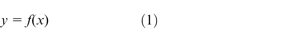
The cutting edge shape of industry standard scalpel blades can be expressed as continuously differentiable polynomials, f(x), as shown in Figure 3 and equation (1). Here, x is the cut depth of the scalpel blade measured from the scalpel tip, point O. The y-direction is perpendicular to the x-direction and is also the cutting direction of the blade when used in slide cutting. The unit vector in the y-direction is v (x) = {0, 1, 0}. The unit vector in the x-direction is c (x) = {1, 0, 0}. The vector tangent to f(x) is $s(x)=\{1,|f\prime (x)|,0\}$ (see Figure 3)

$$y=f(x)$$

(1)

Figure 3.

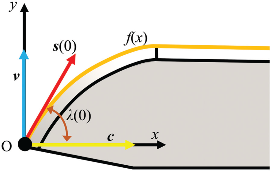
Coordinate system and vectors used in the geometric model to define the inclination angle of scalpels.

The inclination angle is a function of x, λ(x), and is defined as the angle between the P_r plane and the s (x) vector as shown in Figures 3 and 5.^16,17 The P_r plane has the normal vector v (x). Therefore, the inclination angle can be solved as the complimentary angle between v (x) and the s (x) as shown in equation (2)

$$\sin \left(\lambda \left(x\right)\right)=\frac{|\mathit{s}(x).\mathit{v}(x)|}{\left||\mathit{s}(x)||\mathit{v}(x)|\right|}$$

(2)

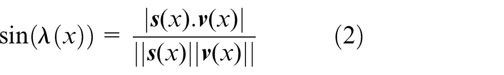
On solving equation (2) explicitly for λ(x) and substituting the values for s (x) and v (x) vectors, equation (3) is produced

$$\lambda \left(x\right)={\sin }^{-1}\left(\frac{|f\prime (x)|}{\sqrt{1+{|f\prime (x)|}^2}}\right)$$

(3)

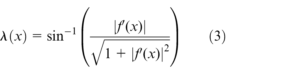
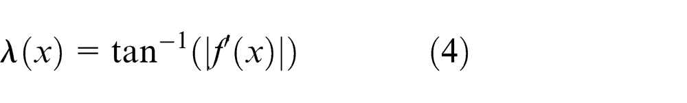
This expression can be further simplified as an inverse tangent of the absolute value f′(x) as shown in equation (4)

$$\lambda \left(x\right)={\tan }^{-1}\left(|f\prime \left(x\right)|\right)$$

(4)

Normal rake angle of scalpel blades

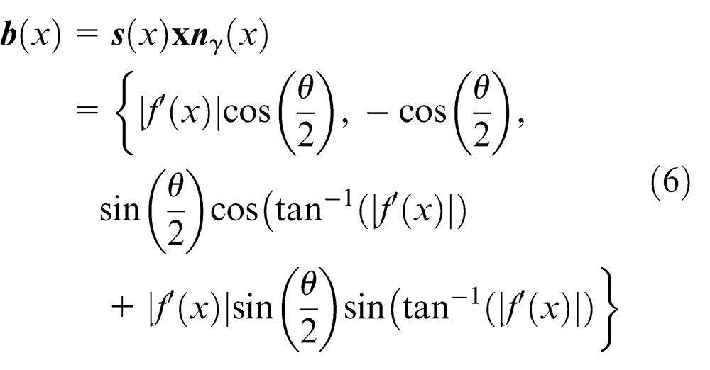
The definition of a tool normal rake angle is the angle between plane P_r and A_γ measured in plane P_n when the bottom rake face acts as the reference plane as shown in Figure 4 with vectors a ′(x) and b (x).^16,17 However, the x–y plane has been used as the reference in this study for simplifying the analysis. Thus, the normal rake angle has been computed by finding the angle between vector a (x) and vector b (x), where a (x) is the cross product of s (x) and v (x) as shown in equation (5) and b (x) is the cross product of s (x) and n_γ (x) as shown in equation (6), where ${\mathit{n}}_{\gamma }(x)=\{-\sin (\theta /2)\sin ({\tan }^{-1}(|f\prime (x)|)),\sin (\theta /2)\cos ({\tan }^{-1}(|f\prime (x)|)),\cos (\theta /2)\}$ and $\theta (x)$ is the angle ground into the cutting edge, which is the normal rake angle of the blade overestimated by a value of $\theta /2$ as shown in Figures 4 and 5

$$\mathit{a}\left(x\right)=\mathit{s}\left(x\right)\mathbf{x}\mathit{v}\left(x\right)=\{0,0,1\}$$

(5)

$$\begin{array}{cc}\multicolumn{1}{c}{\mathit{b}\left(x\right)}& =\mathit{s}\left(x\right)\mathbf{x}{\mathit{n}}_{\gamma }\left(x\right)\hfill \\ \multicolumn{1}{c}{}& =\{|f\prime \left(x\right)|\cos \left(\frac{\theta }{2}\right),-\cos \left(\frac{\theta }{2}\right),\hfill \\ \multicolumn{1}{c}{}& \sin \left(\frac{\theta }{2}\right)\cos ({\tan }^{-1}\left(|f\prime \left(x\right)|\right)\hfill \\ \multicolumn{1}{c}{}& +|f\prime \left(x\right)|\sin \left(\frac{\theta }{2}\right)\sin ({\tan }^{-1}\left(|f\prime \left(x\right)|\right)\}\hfill \end{array}$$

(6)

Figure 4.

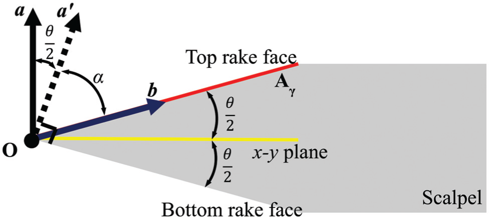
Cross section of scalpel blade displaying the vectors used in the geometric model of the normal rake angle.

Figure 5.

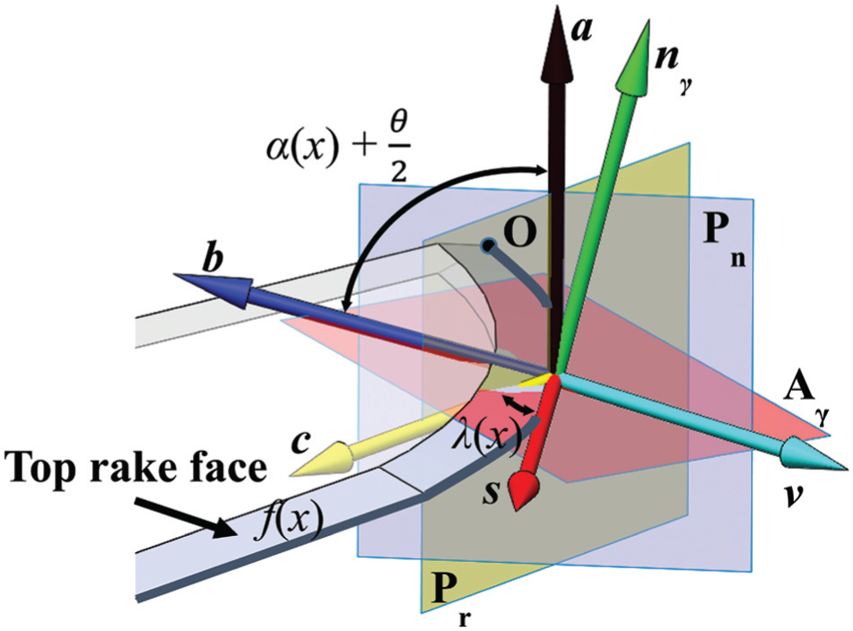
Coordinate system and vectors used in the geometric model to define the normal rake angle of scalpels.

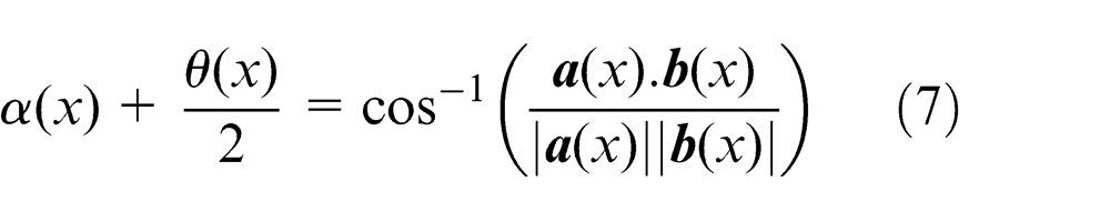
The normal rake angle can be calculated as shown in equation (7). This then simplifies to equation (8) where the normal rake angle is solely dependent on θ(x)

$$\alpha (x)+\frac{\theta (x)}{2}={\cos }^{-1}\left(\frac{\mathit{a}(x).\mathit{b}(x)}{|\mathit{a}(x)||\mathit{b}(x)|}\right)$$

(7)

$$\alpha (x)=90-q(x)$$

(8)

Contact surface area

Scalpel blades with different geometries have different surface areas in contact with tissue during cutting for a given cut depth (x). The total tissue cutting force (F_t ) can be decomposed into tissue stiffness force (F_s ) and tissue friction force (F_f ) as shown in Figure 6. The stiffness force of the tissue varies between 0 and the tissue rupture force. When a tissue cutting instrument initiates contact with the tissue, the tissue will deflect until the rupture force is reached and tissue cutting occurs. ¹⁷ The friction force is primarily dependent on the amount of surface area in contact with the tissue. There are numerous analysis techniques available to determine the surface area of the scalpel in contact with tissue during the cutting process. However, in this study, accurate three-dimensional CAD models were developed for the scalpel blades being studied. These models were then used to evaluate A(x) based on x (see Figure 6).

Figure 6.

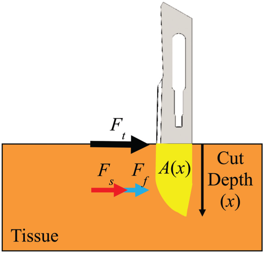
Force decomposition and contact area between scalpel and tissue during slide cutting.

Phantom gel slide cutting experiment

A scalpel cutting experiment was developed to investigate the relationship between cutting forces and the geometry of the 10, 11, 12, and 15 scalpel blades. The experiment consisted of a scalpel blade cutting through phantom gel in a linear, single axis direction at a fixed initial cutting depth to determine the overall cutting force. The setup for the experiment is displayed in Figure 7. The experimental setup comprises a linear motor (Dunkermotoren, Germany), a 6-degree-of-freedom (DOF) force sensor (Nano17 from ATI Industrial Automation, NC) mounted on a lead screw driven translating base, a scalpel holder, a rigid stand and a clear polycarbonate base that restrains the phantom gel while testing. For all experiments, a phantom gel was made of polyvinyl chloride modified with plastisol with a 5:1 ratio of plastic to softener (M-F Manufacturing Company). This material has been used previously as a consistent phantom material to simulate soft tissues inside the body.^13,18 The 5:1 ratio produces a measured material Young’s modulus of 3.6 Pa which is in the range of normal healthy fat tissue, 3.25 ± 0.91 kPa, that is commonly found throughout the body such as in the breasts. ¹⁹

Figure 7.

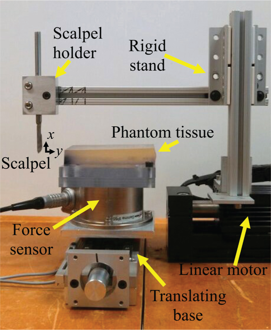
Experimental setup for slide cutting of phantom gel.

Surgical carbon steel scalpel blades made by Havel (Cincinnati, Ohio) (see Figure 1) were mounted on a scalpel holder, and the linear motor propelled the blade through the phantom gel material. The x-axis of the scalpels formed a 90° angle with the cutting direction (y-axis) in all the tests performed. The initial cutting depth was set to 6 mm. A LabVIEW computer code was written to precisely control the cutting speed at 2.54 mm/s. All the phantom gel samples were constrained at the bottom surface by the means of double-sided tape to provide consistent boundary conditions which is crucial for repeatable machining results as illustrated by Shih et al. ²⁰ in machining elastomers.

A total of 12 trials were conducted, 3 trials for each of the 4 blades. The cutting force and cutting depth were recorded. The phantom gel samples dimensions were 119 × 66 × 19 mm. The first cut was made 20.3 mm from the edge of the sample, and two successive cuts were made 12.7 mm apart from the first cut allowing for three test cuts per cutting sample. This minimized boundary effects and isolated each cut from the previous cut, thus improving the consistency of the tests.

Analysis and results

Analysis of cutting tool dimensions

The first step in determining the geometry of the blades is to be able to describe the cutting edge of the blade in terms of a continuously differentiable function, f(x) as shown in equation (1). This was accomplished using image-processing techniques that trace the exterior boundaries of objects as shown in Figure 8. These pixilated data are converted to length measurements, which can be done by dividing the number of pixels in a known length (n_L ) on the blade by the length itself (L). Every pixel coordinate was then divided by the ratio $n_L/L$ to convert the pixel data to length data. The origin, O, was placed at the tip of the cutting edge of the scalpel blade as mentioned above. Various polynomial fits were used to generate a function that describes the cutting edge of the blade with a high accuracy; R ² values were between 0.997 and 0.999. The polynomials that describe the shapes of the four blades studied are shown in Figure 9 and listed in Table 1. This technique can be extended to any blade with a continuously differentiable cutting edge geometry.

Figure 8.

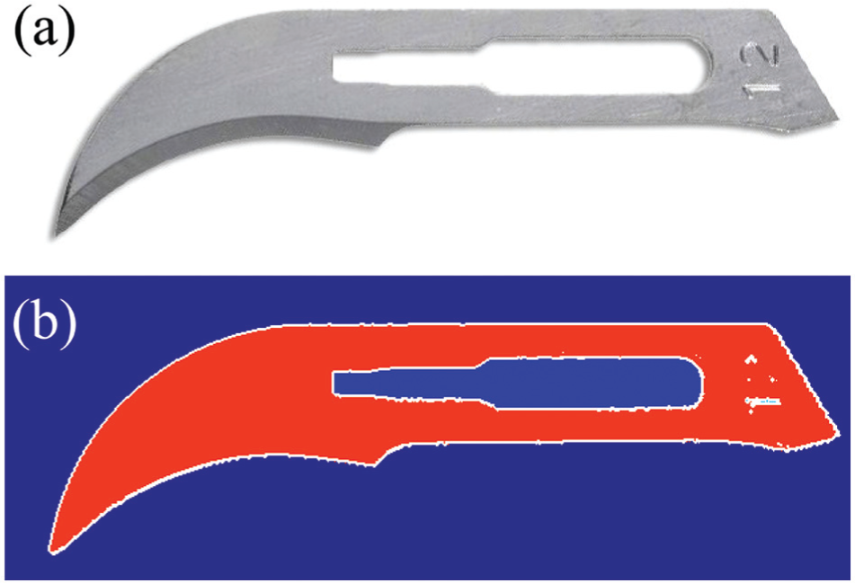
(a) Digital image of scalpel 12 and (b) digitized boundary of scalpel 12 depicted by white pixels.

Figure 9.

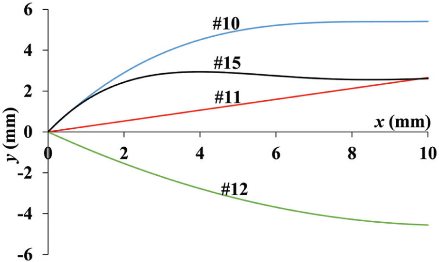
Cutting edge geometry of scalpels used in this study.

Table 1.

List of scalpel cutting edge polynomials and measured ground angles.

Blade	Polynomial f(x) (x in mm)	Average θ±σ(°)
10	7.810 × 10−3 x 3−2.071×10−1 x 2 + 1.831 x	26.43±0.74
11	2.658×10−1 x	14.07±2.40
12	3.965×10−2 x 2−8.523×10−1 x	20.39±1.36
15	−1.313×10−3 x 4 + 4.119×10−2 x 3−4.509×10−1 x 2 + 1.964 x	27.53±1.07

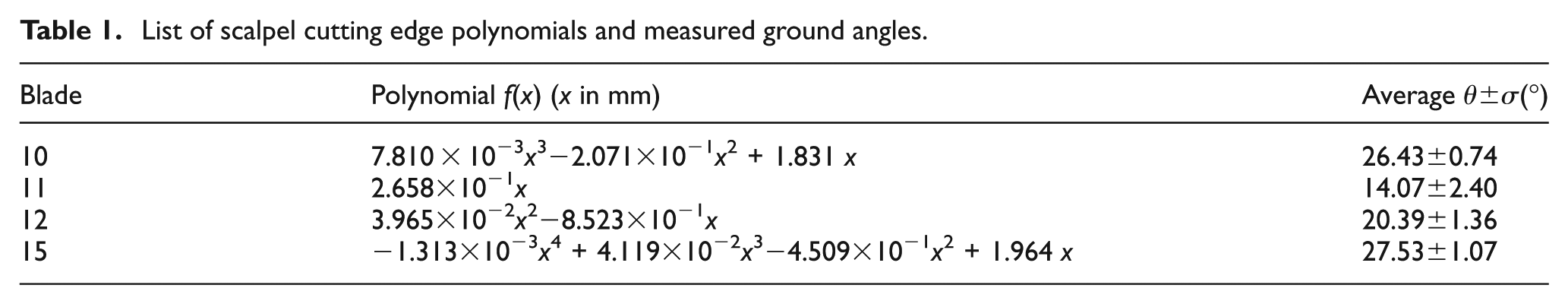
The scalpel blades 10 and 15 have the greatest initial positive slope, while the scalpel blade 11 has the smallest slope magnitude. The scalpel blade 11 displays a constant slope on the plot due to its linear cutting edge (see Figure 9). Due to the scythe shape cutting geometry of the scalpel blade 12, it is the only blade examined in this experiment with a negative initial slope. Scalpel blade 15 is the only examined blade that gradually changes its curvature from convex to concave along its cutting edge. This illustrates how geometries of blades can greatly vary and therefore will display a variety of slide cutting characteristics.

The value of θ was measured using a Zeiss Axio optical microscope, and the results are shown in Table 1. This value of θ changed minimally in relationship to x; therefore, it was assumed in the calculations of λ and α that θ was constant.

Analysis of cutting depth

The initial cut depth for all the slide cutting experiments was 6 mm; however, the compliance of the phantom gel caused this value to change continuously as the scalpel cut through tissue. Also, different scalpel geometries led to different amounts of tissue deflection which affects the value of F_t . Thus, to closely estimate the value of the cut depth at each point in the scalpel’s trajectory through the tissue, ink was poured into the top of the cut groove after each cut was complete. Once the ink seeped all the way through the cut and dried, a knife was used to separate a section of the tissue containing the cross section of the scalpel cut which showed up in the dried black ink as shown in Figure 10.

Figure 10.

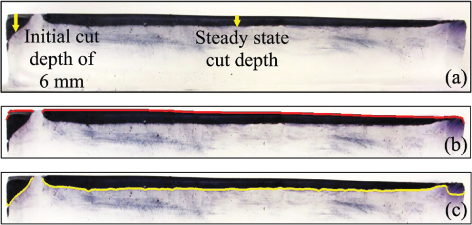
Section of phantom gel showing (a) cut pattern used to estimate cut depth, (b) digitization of top surface of cut pattern, and (c) digitization of bottom surface of cut pattern.

After this, the top and bottom surfaces of the cut were digitized similarly to the previous method used to measure the scalpel cutting surface. After digitization, the pixel data were converted to length data and then the vertical difference between the two curves is the cut depth or x value as a function of cut length (y).

Results of geometric model

The value of $\theta$ has no effect on the value of λ(x) since the two parameters are unrelated; however, it does have a major influence on α(x). A lower $\theta$ and, therefore, a sharper blade leads to an increase in the angle that its normal rake face vector b (x) makes with the vector vertical to the x–y plane a (x) to give higher normal rake angle values.

Equations (4) and (8) are used to calculate λ(x) and α(x) (see Figures 11 and 12). The accuracy of these models was verified using the CAD models developed for the four scalpels. The results of the A(x) were measured using the CAD models of the scalpel blades (see Figure 13).

Figure 11.

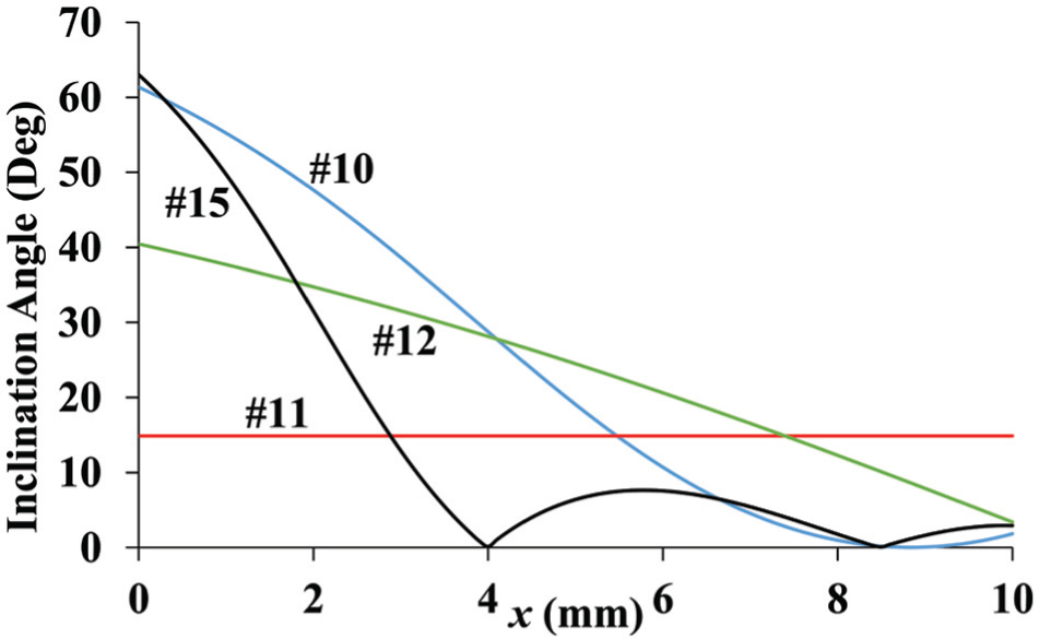
Inclination angle estimation as a function of cutting depth.

Figure 12.

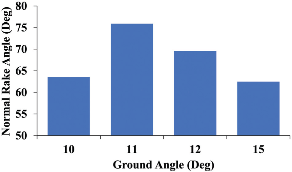
Bar graph of normal rake angle estimation.

Figure 13.

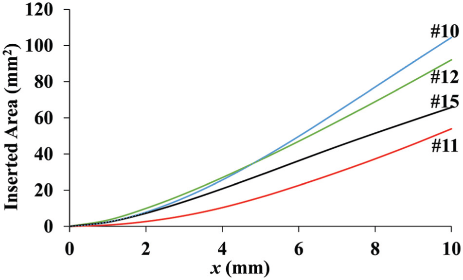
Contact surface area between tissue and scalpel during slide cutting as a function of cutting depth.

Figure 11 displays the inclination angles of all four scalpel blades as a function of cutting depth x. The scalpel blades 10 and 15 have high initial inclination angles at point O (x is zero). However, they also exhibit a steep drop in the inclination angle which quickly reduces to values lower than scalpels 12 and 11 for higher cutting depths. Scalpel 15 reaches an inclination angle of zero at x = 4 mm due to the change in curvature from convex to concave. The scalpel blade 11 shows a zero slope because of its linear cutting edge geometry, giving it a constant inclination angle. For scalpel 12, the inclination angle also decreased, but more gradually compared to 10 and 15.

Figure 12 displays the normal rake angle of each of the four scalpel blades used in this study. A high normal rake angle signifies a sharper scalpel cutting edge surface. Irrespective of the shape of the cutting edge, the normal rake angle for scalpel blades remains constant as it is by definition measured in the plane P_n which always stays normal to the s (x) vector (see Figure 5). Equation (8) captures this behavior as α is only a function of the ground angle or θ which has been assumed to be constant in this study, and hence, α also displays a constant value. Blade 11 displays the highest value of normal rake angle followed by blade 12, blade 10, and finally blade 15 which has the smallest normal rake angle of the four blades studied.

Figure 13 displays the contact surface area of the scalpel blades used in the experiment as a function of cut depth (x). All plots have a similar upward trend as a result of increasing contact surface area as cutting depth increases. At the full 10 mm of insertion, scalpel 10 has the highest contact area followed by scalpels 12, 15, and 11. At x < 4.66 mm of insertion, scalpel 12 has the highest amount of contact area. These differing scalpel geometries result in different contact areas between scalpel and tissue. Scalpels with higher surface area will increase the friction between the scalpel and the tissue and therefore lead to higher F_t values.

Results of slide cutting experiments

Figure 14 depicts the results of the total cutting force averages obtained over the three cuts made per sample in the test method described previously. The varying geometry of the four blades creates unique cutting force profiles for each of the blades. All four graphs have an initial spike as expected due to the fracture mechanism required at the beginning of the cut. However, they all settle to a relatively steady value once x becomes fairly constant by y > 30 mm. Although the initial cut depth was 6 mm for all samples, the average cut depth in the steady force region varied for the four blades based on how their geometry interacted with the phantom gel and the amount of deflection it caused during slide cutting.

Figure 14.

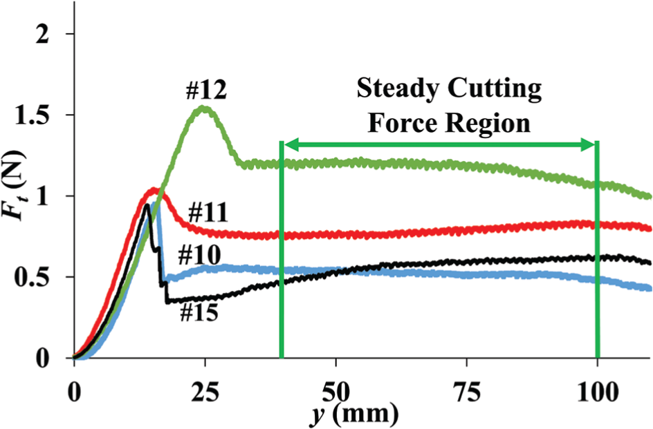
Total cutting force during slide cutting as a function of cut length.

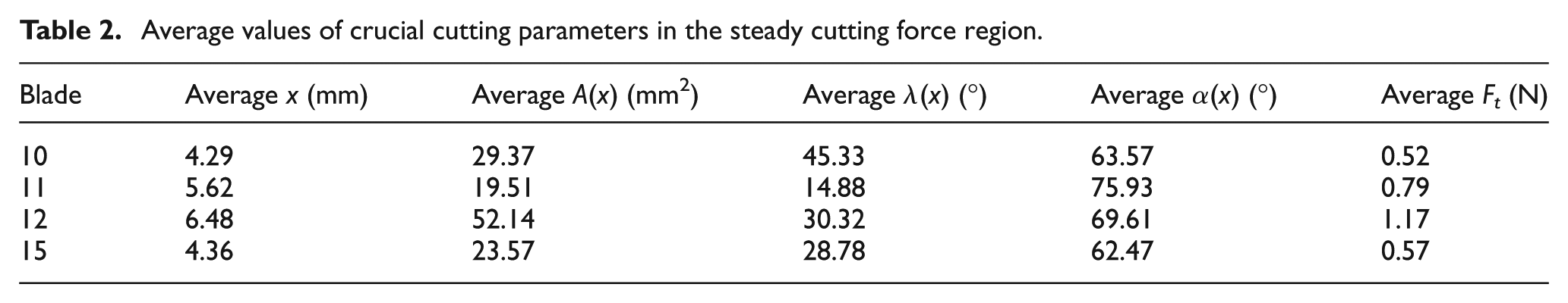
Table 2 depicts the average values of x, A(x), λ(x), and α(x) along cut length values (y) with a relatively steady cutting force region which is taken to be where y is between 40 and 100 mm (see Figure 14). Blade 10 displays the lowest average F_t value followed by blades 15, 11, and 12, respectively. Using the data from the scalpel cut digitization along with the F_t graph, one can normalize the F_t with respect to x as shown in Figure 15. Blade 10 displays the lowest average normalized F_t value of 0.16 N/mm followed by blades 15, 12, and 11 with a value of 0.19 N/mm.

Table 2.

Average values of crucial cutting parameters in the steady cutting force region.

Blade	Average x (mm)	Average A(x) (mm2)	Average λ(x) (°)	Average α(x) (°)	Average Ft (N)
10	4.29	29.37	45.33	63.57	0.52
11	5.62	19.51	14.88	75.93	0.79
12	6.48	52.14	30.32	69.61	1.17
15	4.36	23.57	28.78	62.47	0.57

Figure 15.

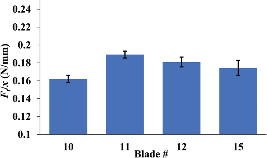
Bar plot of normalized total cutting force with its standard deviation.

In conventional cutting, a lower cutting force is able to be obtained by reducing contact area and increasing normal rake and inclination angle. This trend appears to be true also in scalpel tissue cutting as shown in Table 2. It is shown that blade 10 contains the highest average inclination angle and the lowest average cutting force. Blade 12 contains the highest contact area and the highest average cutting force.

Conclusion

In this study, a generalized geometric model that describes the cutting edge of scalpel blades was developed. This study specifically focused on four industry standard scalpel blades 10, 11, 12, and 15. Analytical solutions to determine the inclination angle and normal rake angle have been found and are expressed in equations (4) and (8), respectively. CAD models of the four blades were developed to estimate the contact surface area between the scalpel and the phantom gel.

Through the results of the analytical expressions developed, it was found that the geometries of the four blades studied have various similarities and differences. It was found that blade 11’s constant sloped profile caused it to be the only measured blade to have a constant inclination angle. The rake angle of the blades varied based only on the ground blade angle. The profile of blade 10 produced the largest surface area when inserted 10 mm followed by blades 12, 15, and 11.

The differences in geometry between the four measured blades resulted in differences in experimentally measured slide cutting force. The experimental results showed that blade 10 displayed the lowest average total cutting force of 0.52 N followed by blades 15, 11, and finally 12 with a force value of 1.17 N. Blade 10 also displayed the lowest average normalized cutting force of 0.16 N/mm followed by blades 15, 12, and finally 11 with a force value of 0.19 N/mm.

Further investigation is required in order to model the relationship between geometric parameters and the cutting force. The generalized analytical solutions developed to calculate the crucial cutting parameters provides for the first time a quantitative technique to compare any scalpel blade cutting geometries.