
Abstract
A large aircraft fuselage panel is commonly composed of a variety of thin-walled components. Most of these components are large, thin and compliant, and they are also prone to some flexible deformation during assembly and remain deformed after assembly. Besides, many different fabrication and assembly manners are adopted in order to guarantee the complicated assembly relationships between each component. The above characteristics often cause large aircraft fuselage panels to exhibit low stiffness and weak strength, thereby inducing deformation during assembly. Since the posture of a large aircraft fuselage panel is commonly evaluated by matching the theoretical and actual positions of the measurement points placed on it, and its assembly deformation is also represented by the position errors of the measurement points, a reasonable measurement point placement is significant for the large aircraft fuselage panel in digital assembly. This article presents a method based on the D-optimality method and the adaptive simulated annealing genetic algorithm to optimize the placement of the measurement points which can cover more deformation information of the panel for effective assembly error diagnosis. By taking the principle of the D-optimality method, an optimal set of measurement points is selected from a larger candidate set through adaptive simulated annealing genetic algorithm. As illustrated by an example, the final measurement point configuration is more effective to maximize the determinant of the corresponding Fisher Information Matrix and minimize the estimation error of the assembly deformation than those obtained by other methods.
Keywords
Introduction
Fabrication and assembly of a large aircraft involves a variety of fabrication and assembly operations. A number of raw materials are machined and fabricated into detail parts, which are then assembled into various levels of structural configurations. Starting with basic assembly of detail parts into simple panels, they are then combined together to produce the fuselage, wings and finally the complete aircraft. 1
An aircraft fuselage is commonly assembled by a plurality of fuselage sections, and the fuselage section is generally joined by several large aircraft fuselage panels (LAFPs) such as lower panels, upper panels and lateral panels. Generally, an LAFP is composed of a variety of thin-walled components such as skins, frames, stringers and clips according to design criteria and technical requirements. Different from rigid structures, most of these components are large, thin and compliant, and they are prone to some flexible deformation during assembly and remain deformed after assembly, which causes the assembly variation. Besides, the complicated assembly relationships between each component involve many different fabrication and assembly manners. Because of these characteristics, the LAFP has the characteristics of low stiffness and weak strength, which usually cause the assembly deformation to exceed the allowable tolerance range and generate a large deviation between the ideal and the actual assembly shapes.
For aviation industries, dimensional integrity is a major quality concern in assembly processes. Therefore, digital positioning and alignment systems (DPASs2,3) are widely applied in modern aircraft assembly. A typical DPAS for the LAFP is shown in Figure 1. In this system, to guarantee the accuracy of the posture of the LAFP, a certain number of measurement points is needed to be placed on the LAFP in advance, then the measurement system controls a laser tracker 4 to measure these points so as to evaluate the deviation between the ideal and the actual postures of the LAFP, which can be used as the reference information for further positioning and alignment. 5 The measurement system transfers the measurement data to the control system via a transmission control protocol/Internet protocol (TCP/IP)-based network. The control system calculates the corresponding trajectory data and moves the numerical control positioners (NCPs) using a field bus.
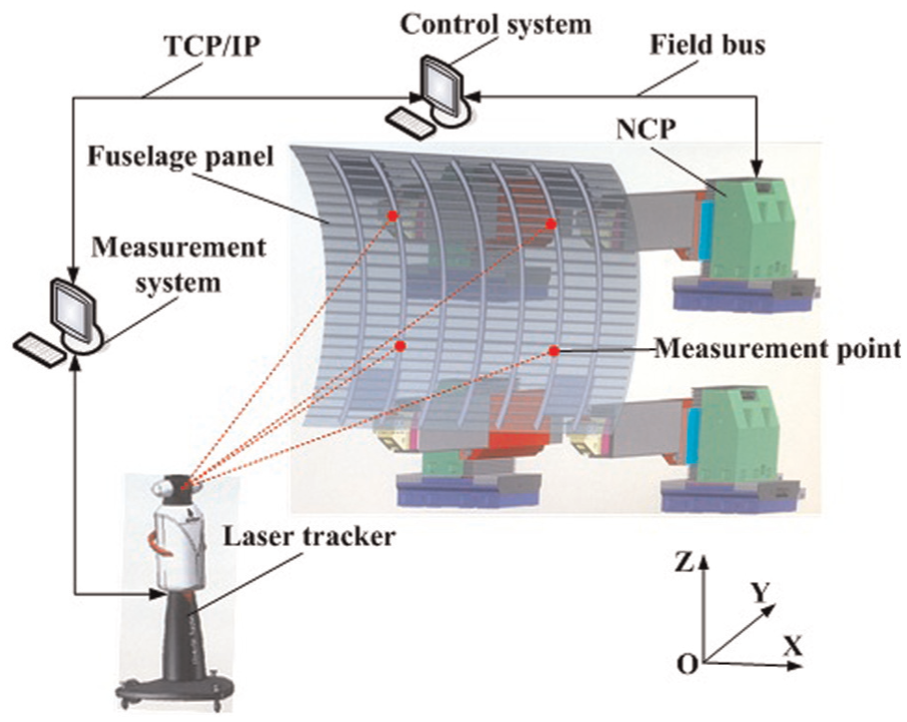
DPAS of an LAFP.
As illustrated in Figure 2, an NCP mainly consists of a chassis, an x-direction slide, a y-direction slide, a z-direction slide and a locating mechanism. The whole NCP is located and fixed on the ground or rigid jigs through its chassis. Each slide is driven by a servo motor, and its current position is fed back to the control system in real time by an absolute encoder. Therefore, an NCP has three translational degrees of freedom (DOFs), and its positioning accuracy in each direction is 0.05 mm. The locating mechanism is installed at the end of the y-direction slide. Non-ideal locating positions of NCPs may lead to the unaccepted assembly deformation of the LAFP. To avoid the quality accidents and dimensional failures of the LAFP, it is necessary to predict the individual contribution of each NCP’s locating variation to the assembly deformation, and appropriate preventive measures, either online or off-line, must be taken accordingly to eliminate the variation sources. For example, Bi et al. 6 proposed an online method to control and correct the assembly deformation effectively by moving NCPs.
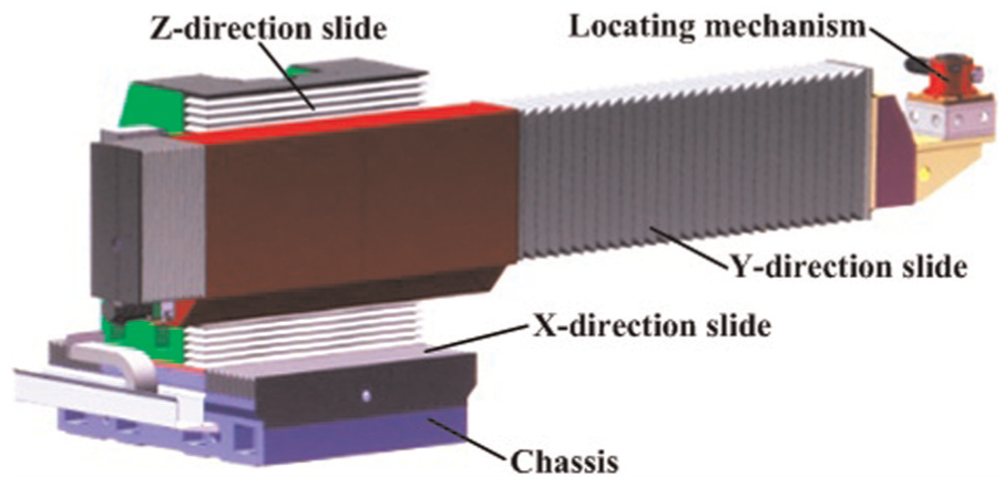
Numerical control positioner (NCP).
In digital assembly, the assembly deformation of the LAFP can be evaluated by the position errors of the discrete measurement points. Different placements of the measurement points generally carry different amounts of assembly deformation information, so how to place the measurement points or choose the positions of product features for the measurement data is very important. An unreasonable placement of the measurement points can adversely affect the accuracy of the posture evaluation and the assembly deformation estimation. For the purpose of covering more deformation information, it is necessary to optimize the placement of the measurement points on the LAFP.
To ensure the dimensional integrity of complex assembled parts, various research efforts have been made into the development of optimal measurement point (sensor) placement methods for assembly processes. Khan et al. 7 and Khan and Ceglarek 8 suggested an optimization method for the sensor locations through estimating a maximal Euclidean distance spread of fault types in space. Ding et al. 9 investigated a strategy for sensor distribution in a multi-station assembly system and presented backward propagation algorithm for the allocation of measurement stations along the process and the determination of the minimal number of sensors within each sensing station. Wang and Nagarkar, 10 Camelio et al. 11 and Jin et al. 12 developed sensor placement methodologies based on the effective independence (EfI) method, which started with a larger candidate set and reached the given number by iteratively deleting those having the least contributions to the linearly independent manifestation of the fixture variations. Liu et al. 13 presented statistical and optimization methods for the coordinate sensor placement for the estimation of the mean and variance components of variation root causes. Liu et al. 14 optimized the sensor placement for fixture fault diagnosis using Bayesian network. However, the objectives of above methods are known to be computationally complex due to their nonlinear characteristics; furthermore, the sensor placement problem becomes even more complex when these objectives are evaluated in a high-dimensional search space. Djurdjanovic and Ni 15 proposed genetic algorithm (GA)-based systematic procedures for synthesizing measurement schemes that carry the most information about the root causes of dimensional machining errors, and they also verified that the new measurement scheme synthesis procedure robustly outperformed the synthesis procedures based on the heuristics of successive measurement removal. Camelio and Yim 16 incorporated a GA-based optimal sensor placement algorithm to determine the key measurement points in assembly, and they found the GA method was significantly faster than the iterative elimination method in Camelio et al. 11 Shukla et al.17,18 presented a feature-based sensor distribution approach for root cause analysis and diagnosis of product variation faults in multi-station assembly processes, the proposed approach integrated state-of-the-art approaches with GA-based procedure for optimal sensor distribution.
As can be seen from the research mentioned above, the optimal placement of the measurement points can not only improve fault diagnosability of assembly variation but also play an important role in assuring the product dimensional or assembly accuracy. For the purpose of guaranteeing LAFP assembly quality, the placement of the measurement points is also needed to be optimized. Because GAs may have a tendency to converge toward local optima or even arbitrary points rather than the global optimum, a method based on the adaptive simulated annealing genetic algorithm (ASAGA) is proposed. The format of the remainder of this article is organized as follows. Section “Modeling for optimal placement of measurement points” establishes the guideline for the optimal measurement point placement based on the D-optimality method. 10 Following this, the strategy for the optimal measurement point placement through the ASAGA is presented in section “ASAGA-based method for optimal measurement point placement.” In section “Case study,” the method is applied to a real LAFP example for verifying its feasibility. Finally, section “Conclusion” draws the conclusions.
Modeling for optimal placement of measurement points
Based on the concept of geometric covariance, 19 it can be assumed that the assembly deformation of the LAFP can be decomposed into the individual contribution of each deformation pattern. Suppose s measurement points are to be placed on the LAFP at s distinct locations, then each deformation pattern can be denoted as follows
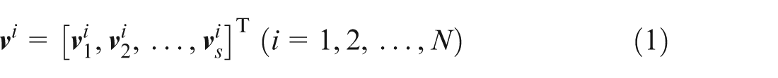
where N is the total number of deformation patterns, and
Now, assume that the sum of the assembly deformation denoted as
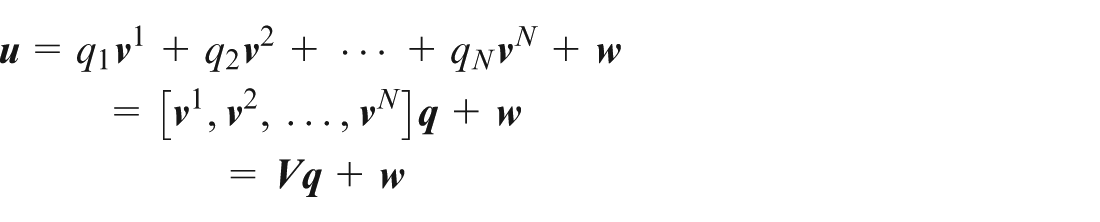
where
As can be seen from equation (2), for obtaining N unknowns,
where
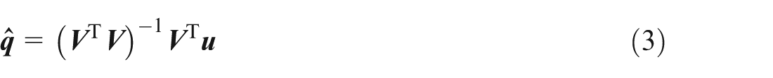
Referring to equation (3), the best set (say, set

For an efficient unbiased estimator, equation (4) can be evaluated by the covariance matrix of the estimate error of
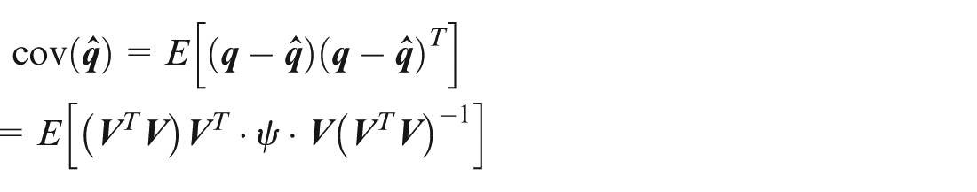
where E[·] denotes the expected value of the quantity in the brackets,
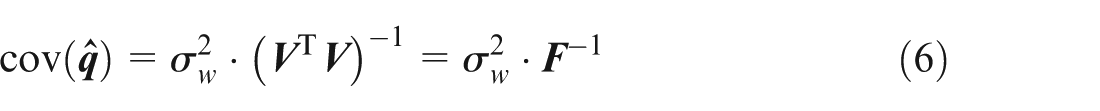
where
According to the EfI method, the EfI of the ith measurement point can be used to represent the fractional contribution of the ith measurement point to the linear independence of the
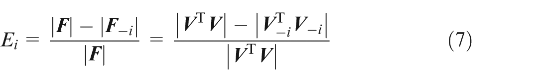
Therefore, in each iterative step, the measurement point which has the lowest value of

where
ASAGA-based method for optimal measurement point placement
GA
GA is a search method based on the principles of natural selection and genetics. 23 In the GA iterative process, the decision variables of a search problem are encoded into finite-length individuals of certain population and then through the operators such as selection, crossover and mutation; the fitter individuals in the current population are stochastically selected and retained to form a new generation, which is further used in the next iteration of the algorithm until a maximum number of generations has been produced or a satisfactory fitness level has been reached.
Fitness function
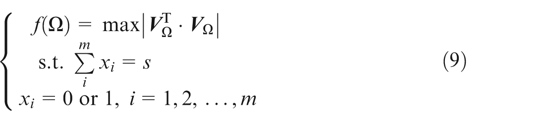
The optimal placement of the measurement points can be regarded as a 0-1 programming problem. 24 If the value of the ith gene is 1, it denotes that a measurement point is placed at the ith location. If the value of the ith gene is 0, it indicates that no measurement point is placed at the ith location. The total number of 1 in a chromosome is equal to the specified number of the measurement points. Suppose the number of initial candidate points is m, and s points are needed to be placed, then the fitness function can be expressed as
Coding and selection schemes
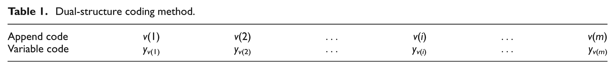
The dual-structure coding method is adopted. As shown in Table 1, the chromosome is composed of two rows, where the upper row v(i) denotes the append code of yj, v(i) = j, and the lower row represents the variable code yv (i) corresponding to append v(i). To code certain individuals, {v(i), (i = 1, 2,..., m)}, list on the upper row, is produced stochastically and then the variable code (0 or 1) is generated randomly. The genetic operators only operate on the upper append code, while the lower variable code is fixed all along.
Dual-structure coding method.
Selection is the process of choosing the fittest individuals from the current population for further operation to yield fitter generation. For the initially generated N individuals, k individuals which are the best ones in current population are defined through the roulette wheel selection scheme. To ensure the diversity, in the residual N–k individuals, the stochastic universal sampling method is adopted.
Crossover operator
The partially matched crossover (PMX) operator 25 is adopted. In PMX, two parents are randomly selected and two random different crossing points are chosen. Alleles within crossing points of a parent are exchanged and swapped with the alleles of another parent.
Mutation operator
The mutation is a random process whereby alleles within a chromosome are changed; it guarantees the diversity of a population and thus reduces the chance that the optimization process becomes trapped in a local optimal region. The swap mutation is adopted herein.
Evolutionary reverse operator
To improve the local search ability of GA, multiple times of evolutionary reverse operators are introduced after mutation, where “evolutionary” refers to the characteristic of the single direction of the reverse operator, that is, only the reverse that improves the fitness values are valid, otherwise invalid.
Adaptive mechanism
In order to vary pc and pm adaptively in response to the fitness values, pc and pm are increased when the population tends to get stuck at a local optimum and decreased when the population is scatter in the solution space. 26 Assume the range of pc is within [pc min, pc max], and the range of pm is within [pm min, pm max], then the new pc and pm can be calculated as follows
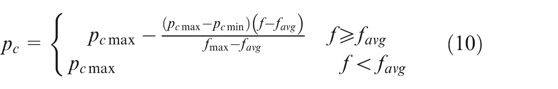
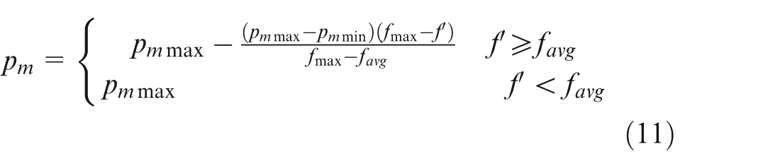
where f is the larger fitness value of the individuals which are to be crossed, f max is the maximum fitness value of the individuals, favg is the mean fitness value of the individuals and f′ is the fitness value of the individual to be mutated.
SA
SA is a random-search technique which exploits an analogy between the way which a metal cools and freezes into a minimum energy crystalline structure and the search for a minimum in a more general system. SA was developed to deal with highly nonlinear problems. 27 The acceptance criteria, initial temperature T 0, final temperature Tf and rules for decrementing the temperature should be specified in SA.
Acceptance criteria
In SA, the candidate solution is accepted as the current solution based on the Metropolis acceptance criterion
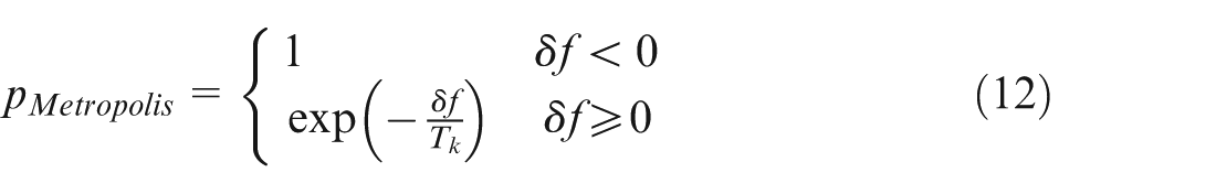
where δf is the increase of the objective function and Tk is the temperature at iteration k.
Initial temperature
A suitable initial temperature T
0 is one that results in an average increase of acceptance probability pr
. The value of T
0 will clearly depend on the scaling of f and, hence, be problem specific. It can be estimated by conducting an initial search in which all increases are accepted and calculating the average objective increase
Final temperature
The stopping criterion can be a suitably low temperature Tf or when the system is “frozen” at the current temperature (i.e. no better or worse moves are being accepted).
Temperature decrement
The simplest and most common temperature decrement rule is as follows

where q is a constant, and its value is usually between 0.8 and 0.99.
ASAGA
Both of GA and SA search a solution space through a sequence of iterative steps. GA mechanism is parallel on a set of solutions, exchanges information using the crossover operator and uses the same selection strategy during the run of the algorithm, while SA works on a single solution at a time and regulates the temperature parameter to evaluate the solution. The differences between the two algorithms lead to different search criteria, and both of them have advantages and disadvantages. A disadvantage of GA is that it might be trapped at local minima, or it is time-consuming to find an optimum solution. In case of SA, only one candidate solution is used; thus it is slow and cannot build up an overall view of the search space, but it can effectively avoid becoming trapped in local minima, while GA has the advantage of discovering the search space rapidly but has difficulty in finding the exact optimum solution. In this study, ASAGA is proposed, which combines the advantages of GA and SA in order to improve the quality of solutions and reduce execution time. The whole flow chart of ASAGA is shown in Figure 3.
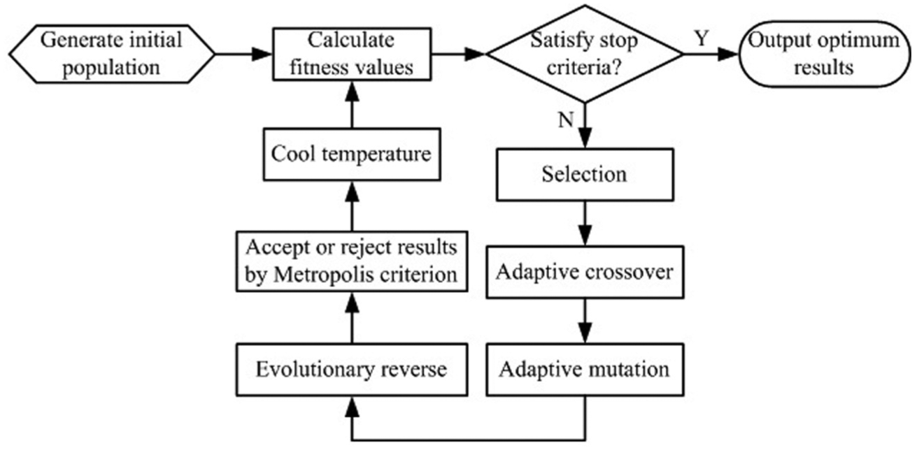
Flow chart of ASAGA.
Case study
LAFP model
A lateral fuselage panel of a large transport aircraft is selected as an example to verify the proposed method for the optimal placement of measurement points in digital assembly. Generally, in the structure of an LAFP, there is no joint reserved for NCPs, so load-transmitting devices (LTDs) (Figure 4) are designed for the transitional connection between the LAFP and NCPs (Figure 5(a)). As can be seen in Figure 4, an LTD comprises a connection body and a ball-head, and there are several bolt holes and hoisting holes in the connection body. The bolt holes are used to install high-strength shear bolts which locate the LTD and bond it tightly with the outer surface of the LAFP (Figure 5(b)), while the hoisting holes are reserved for mounting lifting pins to transfer the panel in each assembly station. As shown in Figure 5(c) and (d), the ball-head is used to form a spherical hinge joint with the ball-socket of the locating mechanism mounted on the NCP. The locating mechanism can keep the ball-head in the ball-socket in an unescaped state by a locking motor, where the ball-head can rotate freely only in the ball-socket (Figure 5(d)). Through the multiple hinge joints between LTDs and NCPs, the LAFP is located and supported finally.
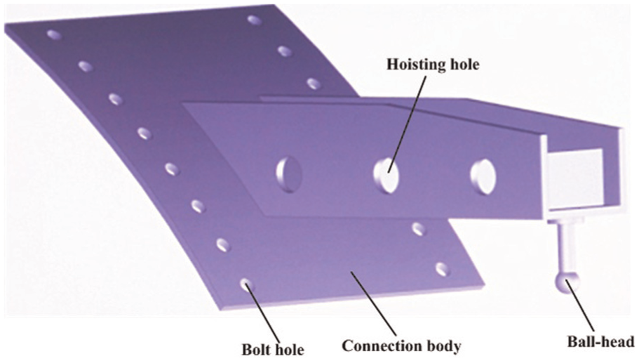
LTD structure.
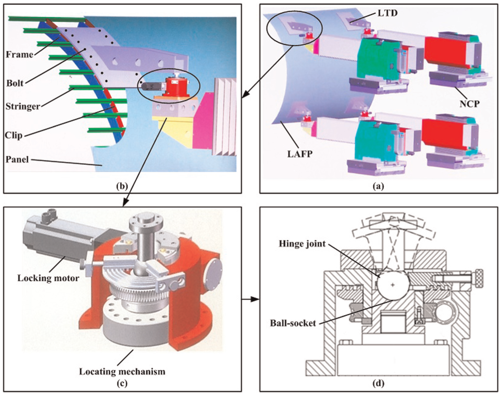
Locating mechanism. (a) DPAS (b) LAFP structure (c) Isometric drawing of locating mechanism (d) Cutaway view of a locating mechanism.
Strictly speaking, in the DPAS, there are many factors that can generate effects on final assembly results. However, in actual assembly processes, before transferring the LAFP from other stations to the assembly station for digital positioning and alignment, some assembly requirements such as the shape and size of the LAFP and the joining must be satisfied. Therefore, in the DPAS, the most important factors that can induce deformation patterns are the non-ideal locating positions of NCPs. In this article, only the deformation patterns due to each NCP’s locating variation are considered.
As depicted in Figure 6, the length of the LAFP in the x-direction is 4260 mm, and the span of the LAFP in the z-direction is 3400 mm. The number of the frames indexed from I to VII along the x-direction is 7, and the number of stringers along the circumferential direction is 26.
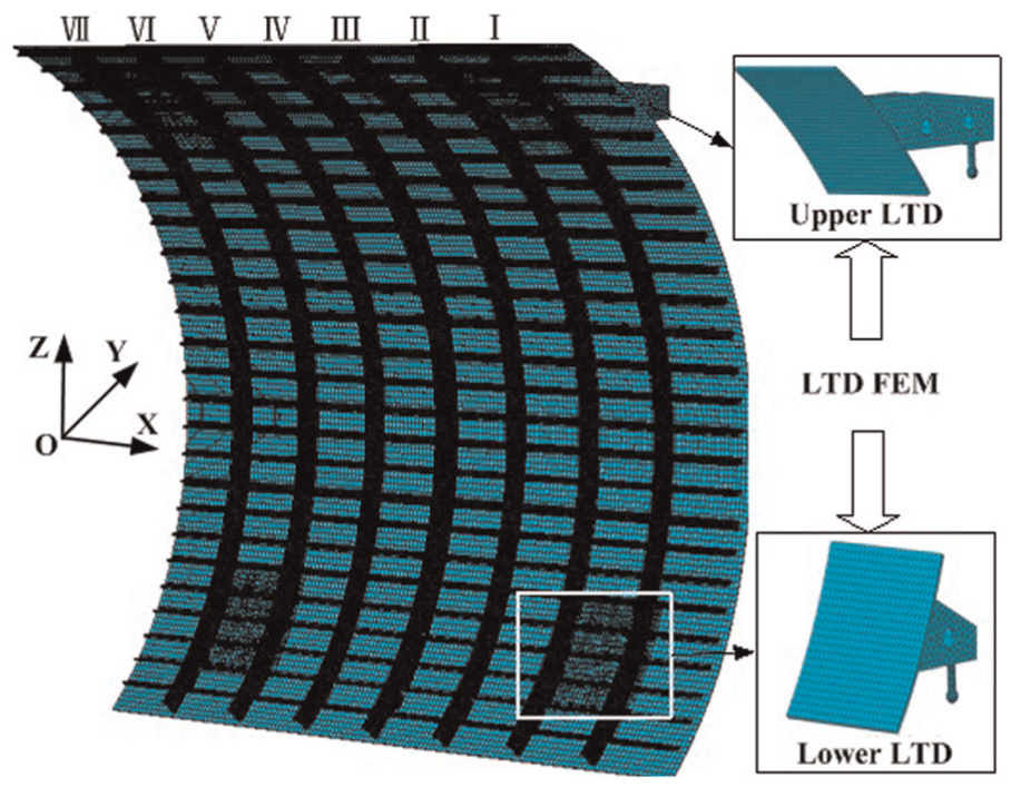
FE model of the LAFP.
To obtain the optimal measurement point placement of this case, the FE model of the LAFP is created using ABAQUS CAE 28 as the pre-processor. All components of the LAFP are modeled by C3D8I elements, and the total number of grid units in the whole model is about 329,110. Parts of the LAFP are usually connected by rivets and bolts, and the position relationships between each part in assembly remain unchanged. In ABAQUS, a tie constraint can tie two separate surfaces together, so that there is no relative motion between them. This type of constraint is able to fuse together two regions automatically, even though the meshes created on the surfaces of the regions may be dissimilar. Therefore, tie constraints are adopted and imposed between each part.
As the actual structure of the LTD is very complex, C3D10M elements are adopted to mesh the grids of each LTD. The LTD is usually connected tightly with the panel by a set of bolts, which can guarantee there is no relative motion between the LTDs and the LAFP. In view of this, using the similar method adopted in panel modeling, the mechanical joints between the LTDs and LAFP can be approximated with tie constraints in order to keep their relative positions unchanged. The axial span and circumferential span of the LTD always contain two frames and four or five stringers, respectively. The material physical and mechanical property parameters of the main parts are listed in Table 2.
Physical and mechanical property parameters of the materials.
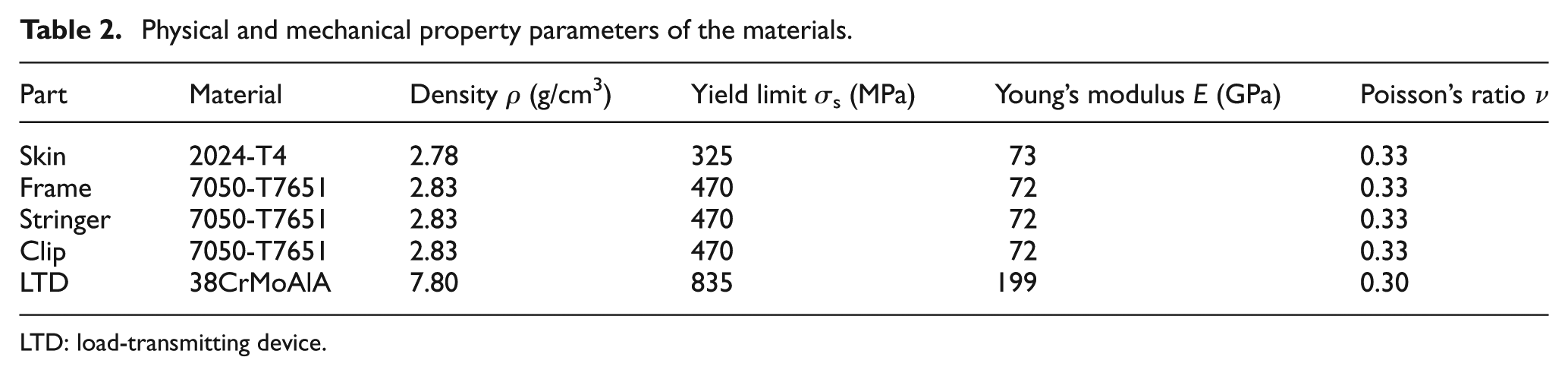
LTD: load-transmitting device.
The LTD is generally designed to be more rigid than the fuselage panel, and its dimension is also smaller than the fuselage panel’s, so each LTD is regarded as a rigid body, and the boundary condition is to establish a reference point in the center of each ball-head, whose translational DOFs in the x-, y- and z-directions are all constrained to simulate the spherical hinge joint between the ball-head of the LTD and the ball-socket of the locating mechanism of the NCP, as shown in Figure 5.
According to the FE model, each deformation pattern can be obtained by loading a unit displacement on the corresponding translational degree of the ball-head; meanwhile, the positioning errors of the initial candidate measurement points can also be obtained.
Initial candidate measurement points
Theoretically, the searching space should contain all nodes of the FE model. However, it is impossible and impractical to select a small quantity of measurement points from a large number of nodes. In practical assembly, the stiffness of frame parts is generally more rigid than that of other parts; frame parts are usually regarded as the assembly benchmarks to sequentially locate and clamp other thin-walled parts such as stringers, skins and clips, exactly coordinating their assembly relationships and guaranteeing the shape accuracy of the LAFP. Therefore, in this article, partial nodes of frame parts are selected as the initial candidate measurement points.
The lateral surface of the frame part, whose normal is the negative x-direction, is used to connect with clips, so that the measurement points are usually placed on its opposite surface. As illustrated in Figure 7, the width of the lateral surface is 64 mm, and spherically mounted retro-reflectors with diameter of 12.7 mm are commonly used to play the roles of measurement points. For the purpose of making a tradeoff between accuracy and economy, the number of initial candidate nodes on a frame part is 50, and the distance between two neighboring measurement points is 70 mm. Thus, the whole model contains 350 nodes as initial candidate measurement points whose indices in the FE model are 225181I−225230I, 622201II−622250II, 623137III−623186III, 624073IV−624122IV, 625009V−625058V, 625945VI−625994VI and 626881VII−626930VII, respectively. The locations of the initial candidate measurement points on Frame I are depicted in Figure 7, while other candidate measurement points’ locations on the rest frames are similar to those on Frame I.
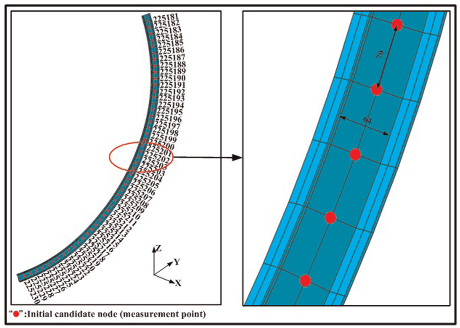
Initial candidate nodes of a frame part.
Parameters of ASAGA
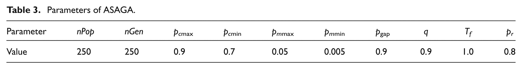
The parameters for running the ASAGA-based method are listed in Table 3, where nPop is the quantity of the population, nGen denotes the maximum genetic generations. nPop and nGen are determined after several test runs. Moderate values of crossover probability (0.5 < pc < 1.0) and small values of mutation probability (0.005 < pm < 0.05) are commonly used. In this article, the parameters for crossover and mutation are pcmax = 0.9, pcmin = 0.7, pmmax = 0.05 and pcmin = 0.005, respectively. pgap denotes the fraction of the population that changes every generation. It has the bounds 0 < pgap ≤ 1. Commonly, pgap = 0.9. q is a constant in the temperature decrement function, and its value is between 0.8 and 0.99. Too large q will decrease the calculation efficiency, while too small q will possibly cause the final result not to be the optimal solution. Therefore, we set q = 0.9 as a tradeoff parameter. T 0 is one that results in an average increase of acceptance probability pr . Generally, pr ranges from 0.6 to 0.99. By referring to Franco, 29 the value of pr is 0.8. It is not necessary to let the Tf reach 0 because as it approaches 0, the chances of accepting a worse move are almost the same as the temperature being equal to 0. Therefore, the stopping criteria can either be a suitably low temperature or when the system is “frozen” at the current temperature. In this article, 1.0 is enough for Tf to satisfy the convergence requirement.
Parameters of ASAGA.
In addition, as can be seen from Figure 5, the LAFP is positioned and supported by four LTDs, that is, there are four NCPs in the DPAS. Therefore, the number of deformation patterns induced by the NCPs is 12. To satisfy the requirement that the matrix
Optimal placement results
Due to the nature of GA method, the results are usually dependent on the randomly generated initial conditions, which mean the algorithm may converge to a different result in the parameter space. For the problem considered in this article, the ASAGA and standard genetic algorithm (SGA) processes have been run for 10 times with a different stochastic initial population.
The ASAGA-based method has been implemented successfully with the parameters listed in Table 3. As can be seen from Figure 8(a), (c) and (e), this method presents a good characteristic of convergence, the best fitness values tend to a constant along with the increasing number of generations, despite lots of fluctuations caused by the search process through the genetic operators such as crossover, mutation and “revolutionary” reverse. From Table 4, it can be observed that for the optimal placement of 20 measurement points, the best fitness value (i.e. the maximum determinant of the FIM) is 5.3436e+04 after 2059 generations, and the computational time is approximately 1876 s; while for the optimal placement of 24 measurement points, the best fitness value is 4.5542e+05 after 2188 generations, and the computational time is approximately 1916 s; the best fitness value of the optimal placement of 28 measurement points is 2.8986e+06 after 1509 generations, and the computational time is approximately 1717 s.
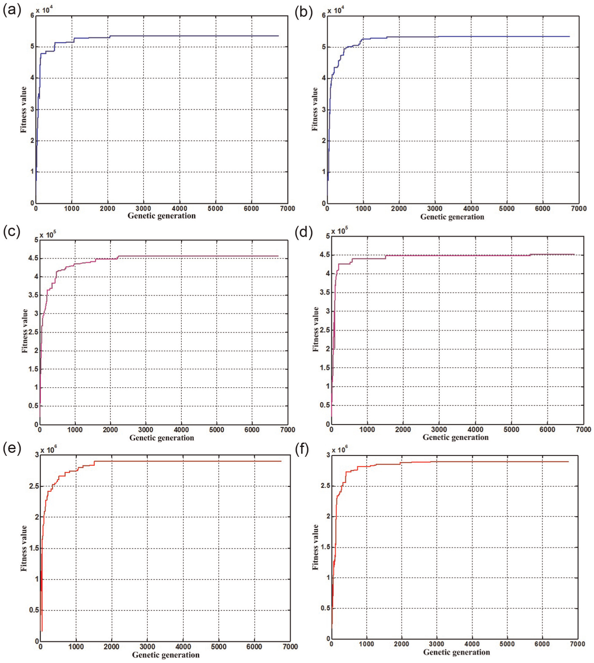
Evolution progress of the best fitness values: (a) fitness value of 20 measurement points using ASAGA, (b) fitness value of 20 measurement points using SGA, (c) fitness value of 24 measurement points using ASAGA, (d) fitness value of 24 measurement points using SGA, (e) fitness value of 28 measurement points using ASAGA and (f) fitness value of 28 measurement points using SGA.
Comparison of results using ASAGA, EfI and SGA.
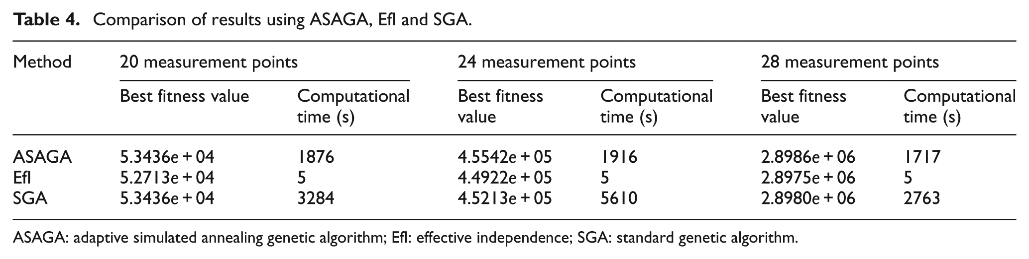
ASAGA: adaptive simulated annealing genetic algorithm; EfI: effective independence; SGA: standard genetic algorithm.
To compare the result obtained by the ASAGA-based method with the results gained by other two methods, in this article, the EfI-based method and the method based on the SGA are adopted, respectively, to get the results under the same conditions.
When adopting the SGA-based method, as shown in Figure 8(b), (d) and (f), the best fitness value of the optimal 20 measurement point placement is 5.3436e+04 after 4221 generations, and the computational time is approximately 3284 s; while the best fitness value of the optimal 24 measurement point placement is 2.8980e+06 after 5523 generations, and the computational time is approximately 5610 s; for the optimal 28 measurement point placement, the best fitness value of is 2.8980e+06 after 2865 generations, and the computational time is approximately 2763 s. If applying the EfI-based method, the maximum determinants of the FIMs of the three cases are 5.2713e+04, 4.4922e+05 and 2.8975e+06 after 5 s, 5 s and 5 s, respectively.
Through comparing the results obtained by the three different methods, it has been demonstrated that the EfI-based method is much faster than other two methods, but its result is relatively poorer than that of other two methods. Although the results obtained by the SGA-based method is close to the result obtained by the ASAGA-based method, it takes more computational time and iterations to estimate the optimal measurement point locations. Therefore, the ASAGA-based method is more effective in solving the problem of the optimal placement of measurement points than other two methods.
The final results of the optimal measurement point placements are listed in Table 5. From Table 5, it can be observed that for the different optimal placements of different numbers of measurement points obtained by the ASAGA-based method, the locations of fewer measurement points are completely included in the locations of more measurement points, and with the increase in the number of measurement points, the maximum determinant of the FIM is also improved, which implies that the deviation between the real deformation and the estimated deformation by the measurement points placed at the locations determined by the ASAGA-based method is also reduced, namely, more measurement points can cover more deformation information. This also shows that the optimization results of different numbers of measurement points have an inheritable characteristic and demonstrates that the convergent result is credible, while for the SGA-based method, the locations of fewer measurement points are not completely included in the locations of more measurement points, which implies that the SGA’s convergent capability is inferior to the ASAGA’s. By comparing the final measurement point placements determined by the EfI-based method and the SGA-based method, respectively, with that selected by the ASAGA-based method, it can be found that for the 20 measurement point placement, there are 1 different point and 0 different point, respectively; for the 24 measurement point placement, there are 1 different point and 3 different points, respectively; and for the 28 measurement point placement, there are 2 different points and 2 different points, respectively. The different nodes are marked in bold in Table 5.
Results of the optimal placements of different numbers of measurement points using ASAGA, EfI and SGA.
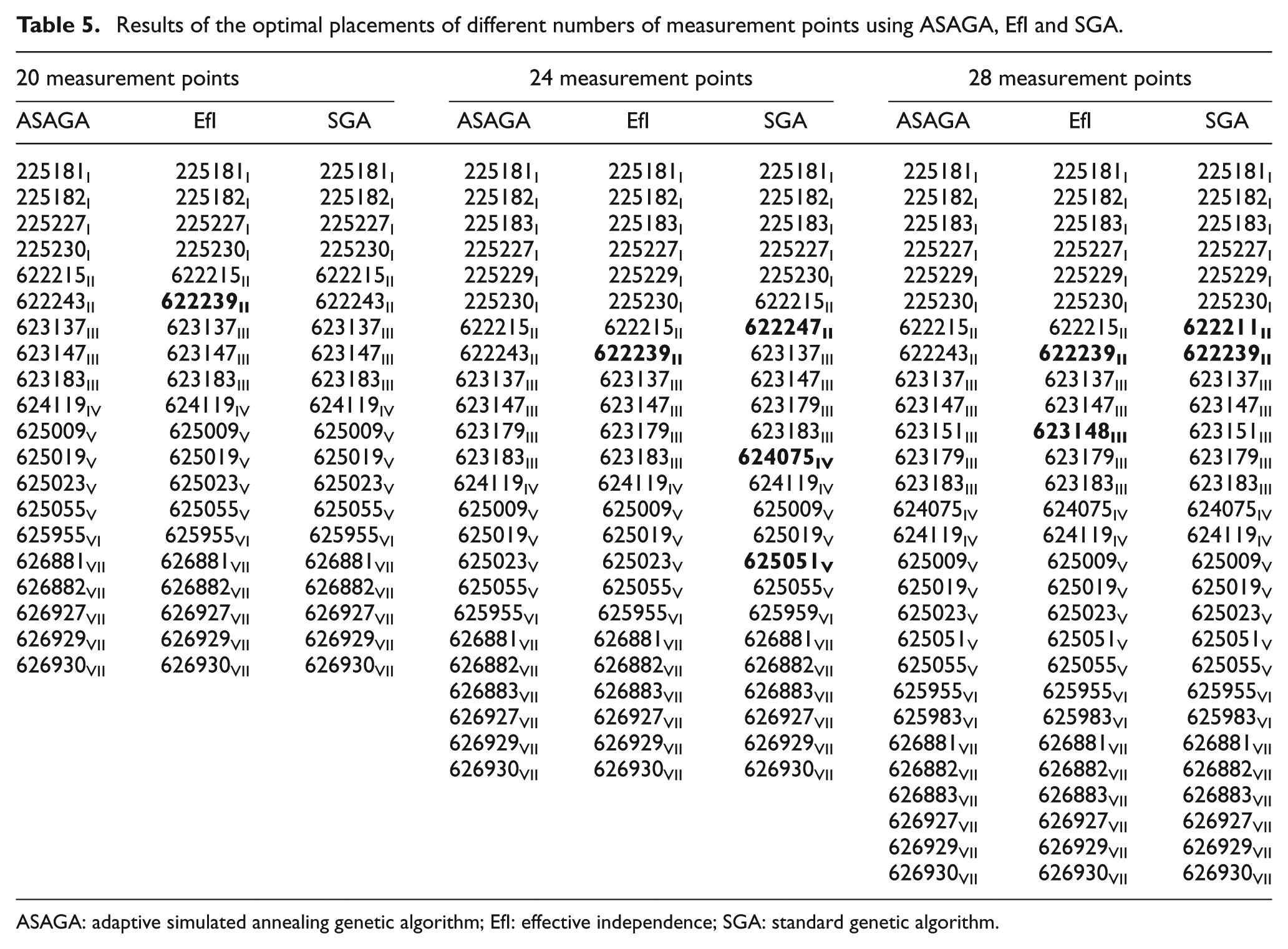
ASAGA: adaptive simulated annealing genetic algorithm; EfI: effective independence; SGA: standard genetic algorithm.
According to the above analysis, to cover more assembly deformation information of the LAFP, more measurement points should be placed at their optimal locations. Therefore, if the conditions such as time and costs permit, enough measurement points are needed to more completely illustrate assembly deformation. For the model depicted in Figure 5, if 28 measurement points are adopted, as can be seen in Table 5, the numbers of measurement points placed on frame parts from I to VII are 6, 2, 5, 2, 5, 2 and 6, respectively.
Conclusion
Ensuring the dimensional integrity of the LAFP has assumed critical importance in modern aircraft assembly. Therefore, it is essential to evaluate the assembly deformation of the LAFP more accurately and completely. The assembly deformation of the LAFP is usually represented by the position errors of measurement points, and different placements of measurement points always cover different assembly deformation information. Aiming at covering more deformation information under the condition that places the same number of measurement points, this article has achieved the optimal measurement point placement on the LAFP through minimizing the estimate error of the assembly deformation. For the purpose of solving the problem of the optimal measurement point placement effectively, the ASAGA-based method has been proposed, which has also been compared with the EfI-based method and the SGA-based method, and the results have shown that the ASAGA-based method is superior to other two methods.
There are many factors that can cause the LAFP to generate assembly deformation, such as the environmental temperature of the assembly workshop, the non-nominal shape and size of parts, the non-nominal location and deteriorated condition of tooling and imperfect joining. Each variation source will lead to a different degree of assembly deformation and ultimately affect the whole aircraft assembly quality. Besides, due to the deformation patterns and initial candidate measurement points determined by the FE model, the modeling errors will also influence the result to some extent. This article optimizes the placement of the measurement points only considering the deformation patterns induced by NCPs, while other variation sources that affect the panel assembly quality are also worthy of in-depth study.
Footnotes
Declaration of conflicting interests
The authors declare that there is no conflict of interest.
Funding
This work was supported by grants from the National Natural Science Foundation of China (No. 51275463) and the Science Fund for Creative Research Groups of National Natural Science Foundation of China (No. 51221004).