
Abstract
The load spectrum is the basis of performing the reliability and fatigue life analysis for the structures of tracked vehicles. In order to obtain the load spectrum, the load cycles should be extracted from the measured or simulated load time history using rainflow counting method. After that, the distribution of the load cycles can be modeled by a continuous distribution function. For the purpose of finding a common modeling method and effective parameters’ estimation method for the load spectrum, we used a mixture of multivariate Gaussian functions to model the probability density function of general load time history on the basis of extracted load cycles. Additionally, we proposed an approach for unknown parameters’ estimation based on variational Bayesian inference. This parameter estimation method can automatically infer the number of components from the observed data set. Numerical examples were given to illustrate the effectiveness of our proposed modeling method and unknown parameters’ estimation method. We compared the distributions of the load cycles reconstructed by the load spectrum models with those of the original load cycles. At the same time, we obtained the quantitative optimal results of the parameters for the load cases. The results showed that the mixture Gaussian functions can model complex distribution of the rainflow load cycles for tracked vehicles by choosing suitable number of components and suitable parameters of them, and the variational Bayesian inference is an effective unknown parameters’ estimation method for the mixture models which have latent variables.
Keywords
Introduction
Tracked vehicles are widely used in the construction machinery and military machinery fields. In the research and development process of tracked vehicles, it is necessary to perform fatigue life analysis for the key structures. At the same time, bench test is an important way to check and improve the quality and performance of the tracked vehicles. Before fatigue life analysis and bench test, we need to accurately predict the loads applied on the structures of tracked vehicles. But the load time history of operating tracked vehicles is a stochastic process. A fragment of measured load time history cannot reflect all the characters of the loads. But the load spectrum can reflect the distribution of the loads. It represents the dynamic loads applied on the structures. 1
In order to determine the load spectrum of tracked vehicles, the load cycles must be extracted from the load time history using suitable counting method. After that, a continuous distribution function should be used to model the distribution of load cycles according to their characteristics. The continuous distribution function is what we called load spectrum. The load spectrum cannot be directly determined by the distribution of load cycles extracted from measured load time history using some counting method. Because of the costs of measurements, the length of measured load time history is usually limited. And the sample data set cannot reflect all the characteristics of the real tracked vehicles’ loads. If the load spectrum is directly determined by the distribution of load cycles extracted from measured load time history. It is not possible to evaluate the influence of the load cycles whose amplitudes and means are higher than those realized in the original measured load time series. This problem is particularly acute when the measured load time series are relatively short. In addition, the distributions of load cycles are different when the load cycles come from different measured load time histories under actual operating conditions. That makes the determination of the load spectrum much more complex. 2 As a consequence of this, the distribution of the load cycles should be modeled by a continuous distribution function.
Because the rainflow counting method takes into account the amplitude and the number of closed hysterias loops simultaneously, it is often used for extracting the load cycles from load time histories. 2 And the load cycles extracted by this method are described in two-dimensional (2D) space. So they have two parameters: the amplitude and the mean, which can be denoted by Y = (Ya, Ym ). In order to model the load spectrum, a proper continuous probability density function (PDF) is often assigned to the extracted load cycles.
Nagode and Fajdiga 2 presented a method of using a multi-model Weibull distribution to model load spectrum. And they developed an unknown parameters’ evaluation method based on histograms of loading frequencies to estimate the parameters of their multiple model. The load spectrum that has more than one basic distribution can be modeled using their method. But because of the solution accuracy, their method cannot model the PDFs of tracked vehicles’ loads very well. Nagode et al. 3 developed a model to simulate random load history by multilayer perceptron. However, it has the shortage of needing much longer load time history. Their method has not been widely used in practice. Furthermore, multi-model Weibull distribution4,5 and multilayer perceptron 6 are not appropriate for modeling most of load time histories
As we all know, the Gaussian has many important analytical properties. It is widely used to model the distribution of continuous variables. But a simple Gaussian has significant limitations and is unable to model the real complex data set. By taking linear combinations of more than one basic Gaussians, we can get the Gaussian mixture model. With a sufficient number of Gaussians, and by adjusting the mean and covariance, as well as the coefficients of the Gaussian components, almost any PDF can be approximated to arbitrary accuracy. 7 Klemenc and Fajdiga 8 applied the mixtures of Gaussian functions to model the different shapes of distribution of the load cycles. They make it possible to describe very different and non-symmetrical PDFs of random variables through application of the mixtures of Gaussian functions. However, the unknown parameters’ estimation is a big problem in this kind of mixture model because of the latent variables. One way to get the estimations of these parameters is the maximum likelihood (ML) estimation method.9,10 Due to the presence of the summation inside the logarithm, we cannot get the closed-form analytical solution by maximum logarithms of likelihood functions. A general approach to find ML estimations for the models which have latent variables is the expectation–maximization (EM) algorithm.11,12 But the EM algorithm cannot detect the proper number of components in the mixture model. We have to select a number of the components in advance. Additionally, the quality of the solution depends on the initial conditions and the number of the components we selected. Furthermore, there will be over-fitting if we choose a large number of components in the mixture models. 13 Markov chain Monte Carlo (MCMC) 14 is another efficient approach to estimate the unknown parameters of mixture Gaussian models. It can use the parameters’ prior distribution information when evaluating the posterior distributions. But the convergence rate of MCMC is relatively slow and the computation is too heavy. 15 It is necessary to develop a general load spectrum model and an efficient unknown parameters’ estimation method for the mixture Gaussian models.
We presented a mixture of multivariate Gaussian functions to model the PDF of tracked vehicles’ load time history on the basis of extracted load cycles or rainflow matrix, as well as proposed an approach for unknown parameters’ estimation based on variational Bayesian inference, which can automatically infer the number of components in the mixture Gaussian model from the observed data set.
Model structure and parameters’ estimation
Load spectrum model structure
The mixture Gaussian distribution is a linear combination of basic Gaussians, which is used to describe the load cycles extracted from load time history of tracked vehicles with rainflow counting method. The PDF can be written as
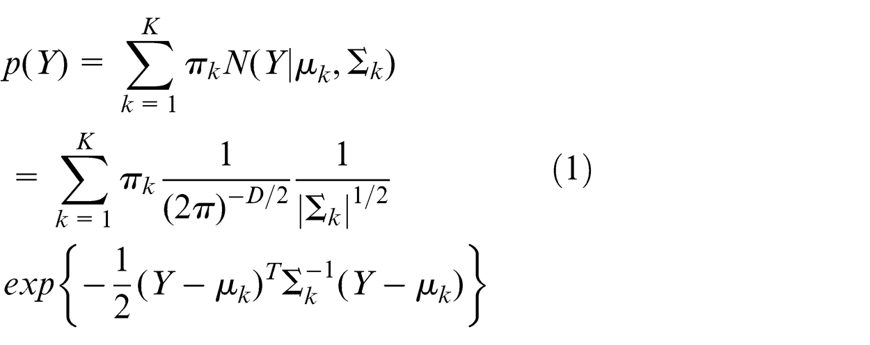
where Y is the 2D random variable which represents the load cycles and Y = (Ya, Ym
); K is the components number; πk
is the mixing coefficient of the Kth Gaussian component, and πk
satisfies 0 ≤ πk
≤ 1 and
Suppose we have a set of observed data
The load spectrum represents the statistical distribution of the rainflow load cycles and is the dependence of entire load cycles’ amplitudes and means. It is obtained from the cumulative density function (CDF) of load cycles. And the load cycle is described by a 2D variable y
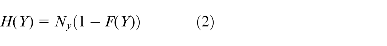
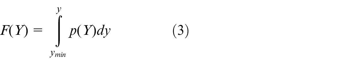
where H(Y) is the load spectrum. Ny stands for the total number of load cycles. p(Y) is the PDF of the load cycles which has the form of equation (1). F(Y) is the cumulative distribution function of the load cycles.
In this mixture model of load spectrum, πk, µk
, and Σ
k
are the unknown parameters.
Variational Bayesian inference
The main task in the process of parameters’ estimation for the mixture model of the tracked vehicles’ load spectrum is the evaluation of posterior distribution of the latent variables given the observed data set (measured or simulated load cycles). Because the posterior distribution has a highly complex form, the evaluation of the posterior distribution is usually infeasible. In such situation, we can rely on some approximate schemes. Bayesian theorem leads us to apply the prior knowledge when calculating the posterior distribution with some new observed data sets. At the same time, the variational inference can provide an approximation method to find approximate solutions in the parameters’ evaluation process. In a Bayesian model, all the latent variables and parameters are considered random variables and given prior distributions. And then, the corresponding posterior distribution can be calculated using the Bayes’ theorem.
Supposing we have a probabilistic model with latent variables and some deterministic parameters. The model has two kinds of unknowns: the latent variables and the parameters. We use vector Z to represent all latent variables and parameters, and
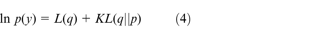
where
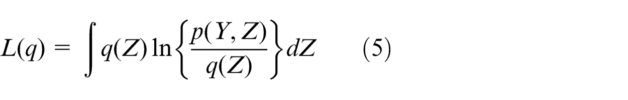
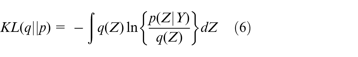
Here, we use integrations in formulating the decomposition, since assuming that Z is continuous. KL(q|p) is the Kullback–Leibler (KL) divergence between q(Z) and the posterior distribution p(Z|Y). KL(q|p) ≥ 0, with equality if, and only if, q(Z) = p(Z|Y). So we can obtain L(q) ≤ ln p(Y), it means that L(q) is a lower bound on ln p(Y).
Notice working with the true posterior distribution directly is intractable in this kind of model. We can change the way and seek a member of the family of distribution q(Z), which is tractable and can provide a good approximation to the true posterior distribution, to minimize the KL divergence. Based on this point, Z can be partitioned into disjoint group and denoted by
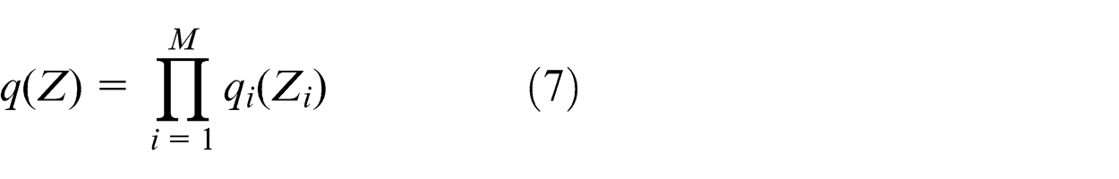
In order to make the algorithm tractable, we make a crucial assumption for the factorization between latent variables and parameters. There is no problem in other factorizations, since the latent variables are i.i.d. on the parameters. Substitute equation (7) into equation (5), we can obtain
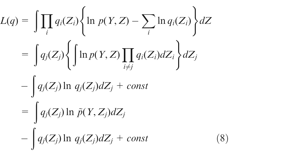
where
In equation (8),
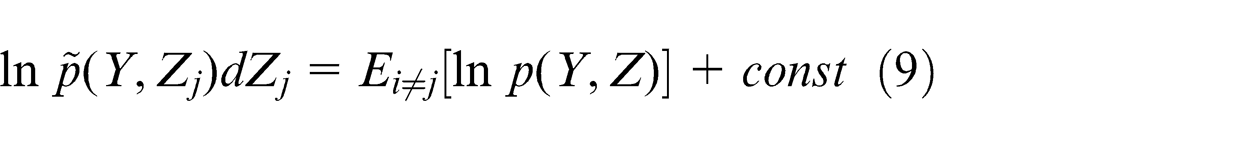
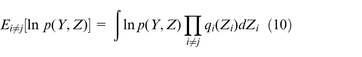
This equation is the basis for application of variational methods. But we cannot use it to get the optimal solution of the lower bound L(q) directly. Because the optimal
Establish an appropriate mixture probability model over observed variables.
Choose an initial setting for all the parameters and latent variables by setting a prior probability over them.
Get a set of observed data.
Cycle over the factors, revising each of them given the current estimations of others until convergence.
Parameters’ estimation for the load spectrum model
In this section, we introduce how to use the variational Bayesian inference to perform unknown parameters’ estimation for the mixture Gaussian model built in section “Load spectrum model structure” over the load spectrum of the tracked vehicles. In order to formulate a variational treatment of the mixture model, we write down the joint distribution of all the random variables including latent variables and parameters in the form of
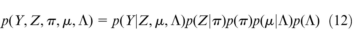
where
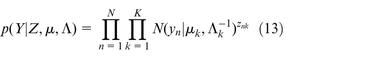
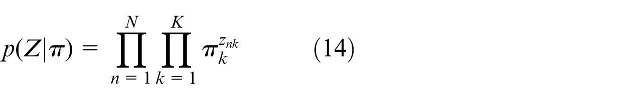
where µk and Λ k are the mean matrix and the precision matrix of the Gaussian component, respectively. znk = 1 if the data point n belongs to the component k, and znk = 0 otherwise.
In equation (12), p(Z|π) is the conditional distribution of the latent variable Z given the mixing coefficient π, and it can be written as
In order to use the prior knowledge in the Bayesian treatment, we assign a prior distribution over each of the parameters in our mixture model. Since the conjugate priors have the same functional forms with the posteriors, as well as it can greatly simplify the Bayesian analysis. We choose the conjugate priors over the parameters µ, Λ, and π.
Therefore, we choose a Dirichlet distribution over the mixing coefficient π
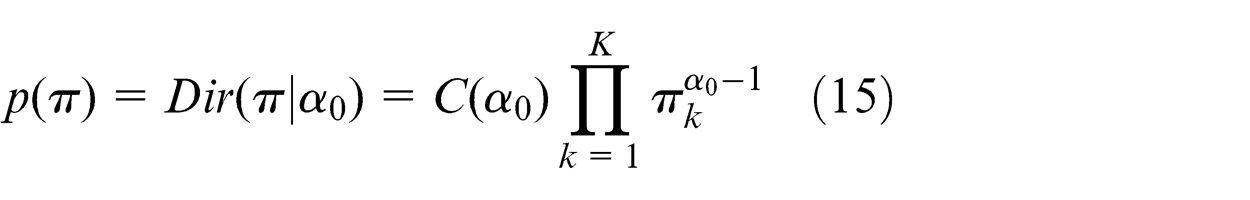
where C(α
0) is the normalization constant for the Dirichlet distribution. And for convenience, we assume that all the coefficients have the same prior. That means
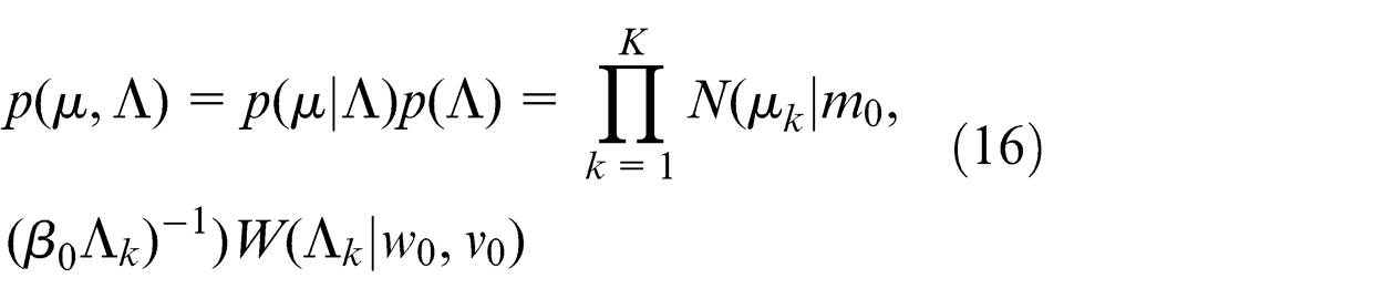
Similarly, we choose an independent Gaussian–Wishart distribution as the conjugate prior distribution over mean and precision of each Gaussian component, which is given by
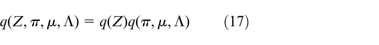
In order to obtain a tractable practical solution to the Bayesian mixture model, we write down a variational distribution which factorizes between the latent variables and parameters
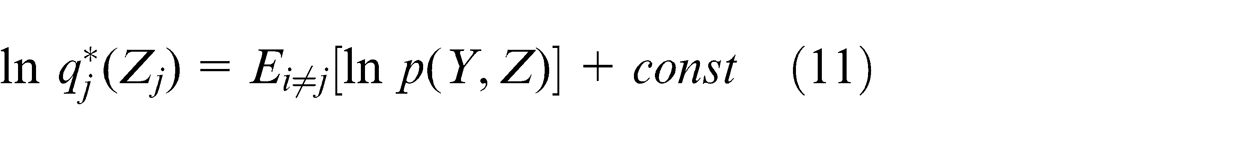
Then, making use of the general optimal result (equation (11)), the log of the optimized factor q(Z) can be given as
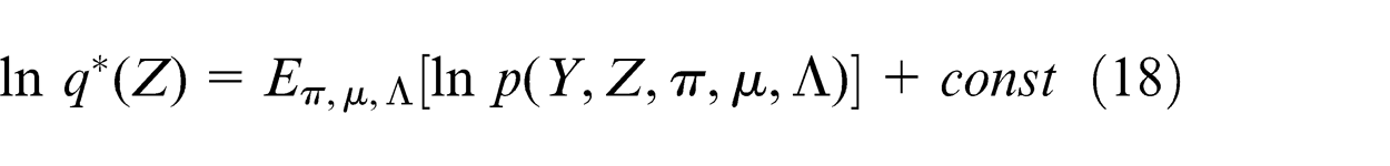
Using decomposition (12) and absorbing the terms that are not dependent on the latent variable Z into the additive normalization constant, the log of the optimal result to latent variables can be written as
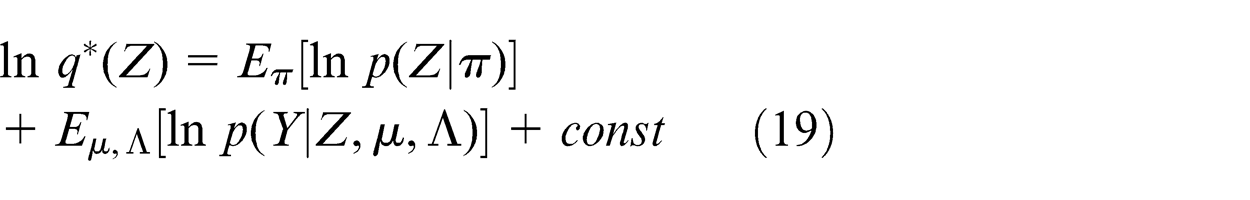
Substituting equations (13) and (14) into the right side of equation (19), and then absorbing the terms that do not depend on Z into the additive constant again, we can obtain
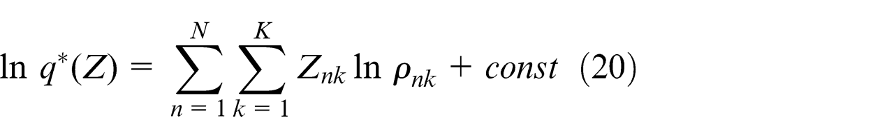
where
D is the dimensionality of the data variable Y (in our case, D = 2). Taking the exponential of both sides of equation (20), we have
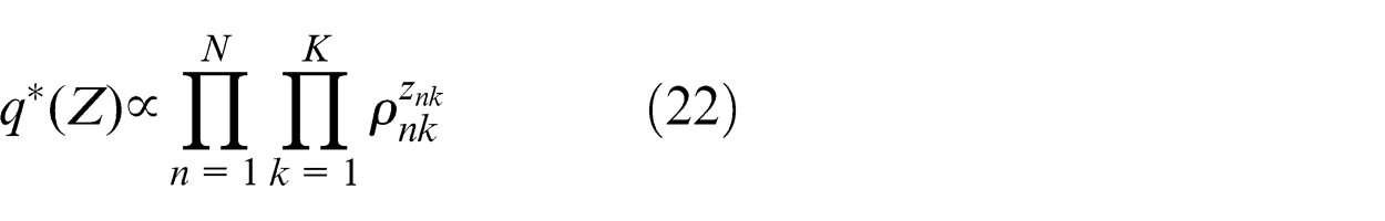
For each value of n, the quantities znk are binary and sum to 1 over all values of k, we obtain
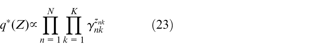
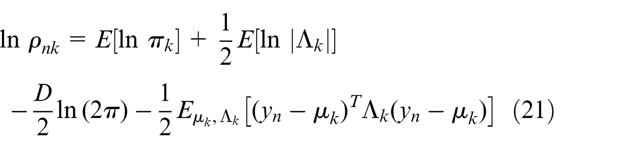
where we defined
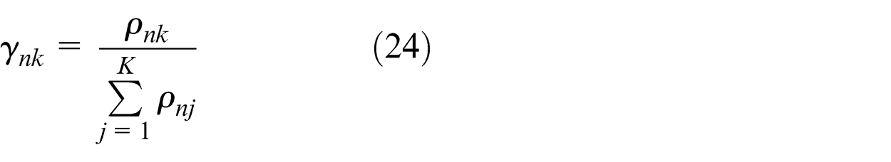
Note that because ρnk is given by the exponential of a real quantity, the quantities γnk will be non-negative and will sum to 1 as required. For the discrete distribution q *(Z), we have the standard result
The quantities ρnk represent the responsibilities. For convenience, we defined three statistics of the observed data set evaluated with respect to the responsibilities, given by
Similarly for the factor q(π, µ, Λ), using the general result (equation (11)), we have
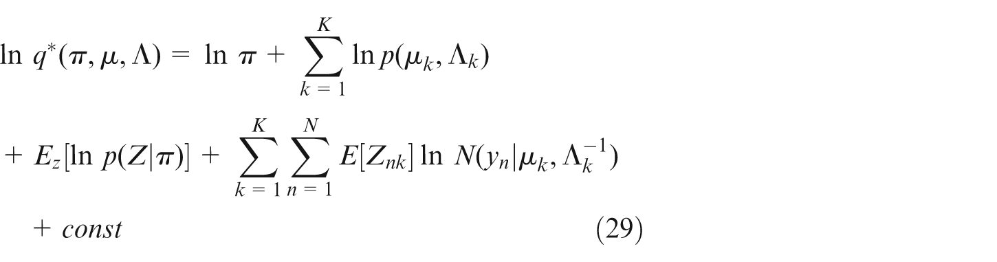
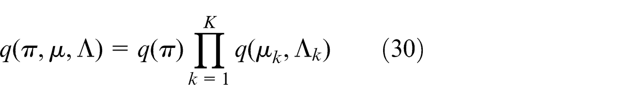
The factor q(π, µ, Λ) has further factorization of
Identifying the terms on the right side of equation (29) that depends on π and using equation (25), we have
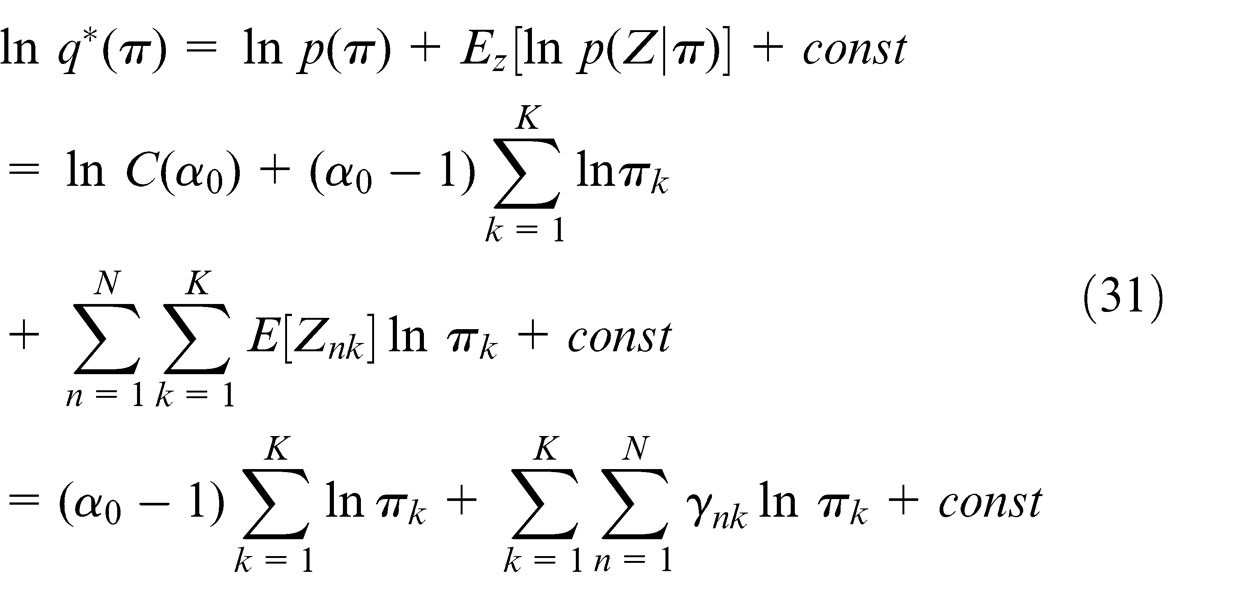
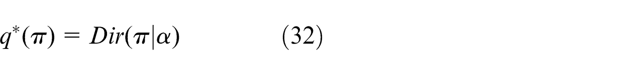
Taking the exponential of both sides and recognizing q *(π) as a Dirichlet distribution, we can write down
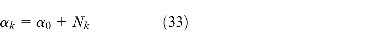
where α has component αk given by
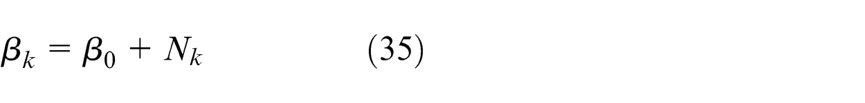
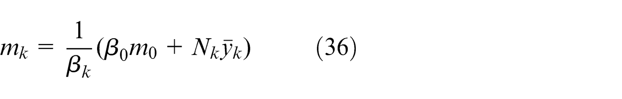
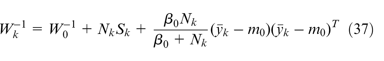
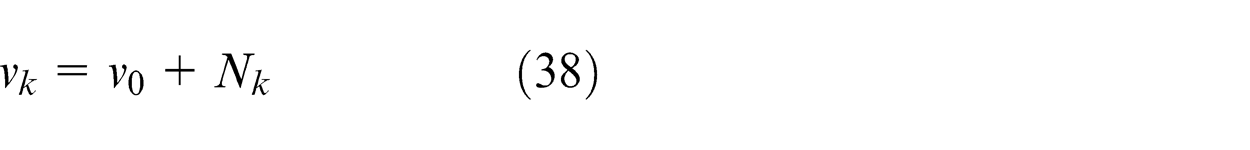
Finally, the variational posterior distribution q *(µk , Λ k ) can be written in the form of q *(µk , Λ k ) = q *(µk , |Λ k )q *(Λ k ). The two factors can be found by inspecting equation (29) and reading off those terms that involve µk and Λ k . The result is a Gaussian–Wishart distribution and is given by
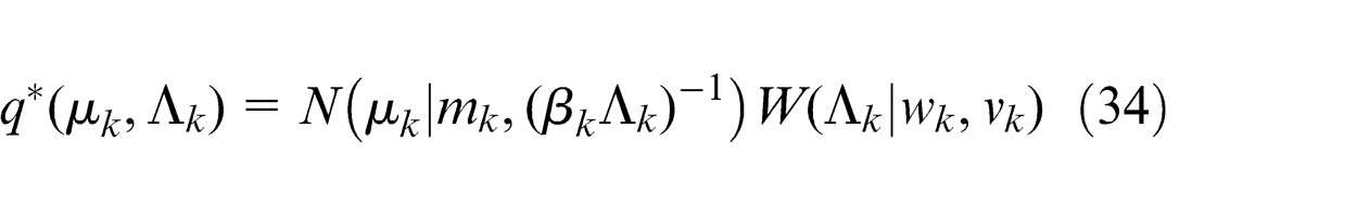
where we defined
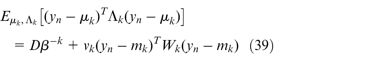
We can see that the update equations (35)∼(38) are similar to the M-step equations of the EM algorithm, and the computations of them need the expectations E[Znk ] = γnk which are similar to the E-steps of EM algorithm. γnk represents the responsibilities and can be obtain by normalizing ρnk which is given by equation (21). Whereas the computation of ρnk involves expectations with respect to the variational distributions of the parameters (Πk, μk, and Σk). At the same time, according to the properties of Gaussian, Wishart, and Dirichlet distributions, we can get the following results
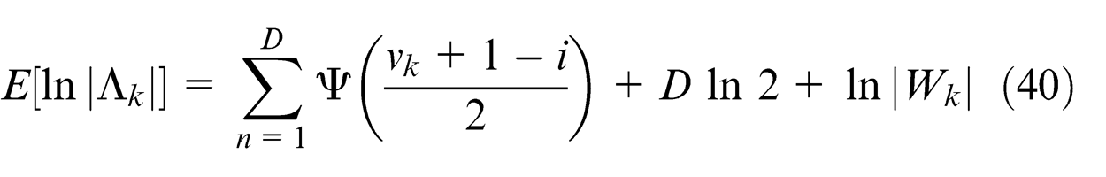
where ψ() is the digamma function, with
Considering the process of evaluations, we can see that the optimal results for the responsibilities and parameters depend on each other. We cannot obtain the closed-form solutions with the optimizations of variational posterior distributions. But we can obtain the approximate solutions by cycling two stages. In the first stage, we use the current distribution over the model parameters to evaluate the parameters with equations (39)–(41). And then evaluate the responsibilities with equation (25). In the second stage, we keep these responsibilities fixed and use them to re-compute the variational distribution over the parameters using equations (32) and (34). This process seems like the E-step and M-step in the EM algorithm. After convergence or the iterations meet the required number, we can obtain a certain precise solution. As for the determination of convergence, it can be considered convergence when the lower bound does not change significantly.
For the variational Gaussian mixture model, the lower bound is given by
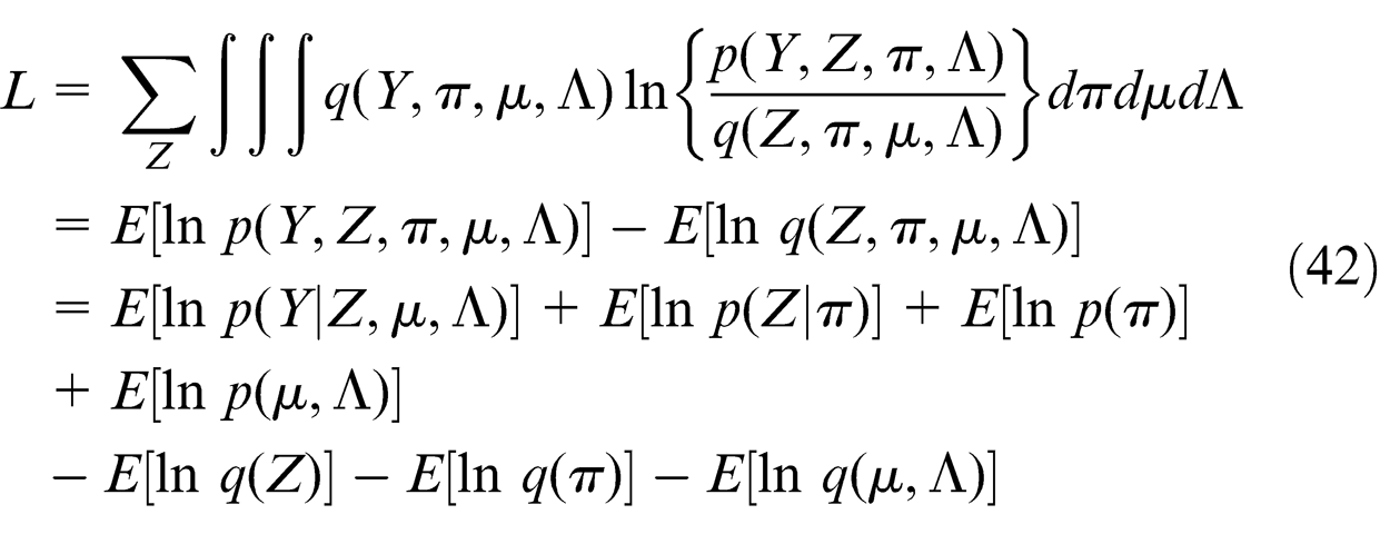
As for the results of the various terms in the lower bound, please refer the study by Bishop. 7 The value of the lower bound should increase monotonically with each step of the iteration. So monitoring the value of the lower bound can help us to test the convergence and check the correctness of the mathematical derivation of the update equations.
In order to determine the suitable value for K, we treat the mixing coefficients π as parameters and make point estimations of their values by maximizing the lower bound with respect to π instead of maintaining a probability distribution over them as in the fully Bayesian approach. The re-estimation equation of πk is given by
This maximization is involved in the variational updates for the q distribution over the remaining parameters. The components that take essentially no responsibility for explaining the data points will have the mixing coefficients driver to 0 during the optimization. At the beginning, we set a relatively large initial value for K, and the superfluous components can be “killed off” from the mixture model through setting the suitable threshold value for πk .
Experiments and results
In order to verify the applicability and the effectiveness of the proposed method for modeling the load spectrum of the tracked vehicles, the simulated and measured rainflow load cycles were used in the following four load cases. We call the load cases that used the simulated rainflow load cycles EXAM_1S, EXAM_2S, and EXAM_3S separately. The load case that used measured rainflow load cycles was named EXAM_4M. The load cycles of traced vehicles in the simulated examples were generated from 2D Gaussian mixture distribution with different parameters.
In order to verify the generalized ability of the load spectrum model and the corresponding parameters’ estimation method, we set the component numbers of the mixture model as 2, 3, and 5 in the three simulated load cycle cases, respectively. Meanwhile, for the purpose of convenience, we assume that the single Gaussian component has the same weight coefficient in the same simulated load cycle case. The mean and covariance matrix are not very important and they are set arbitrarily.
In the load case EXAM_1S, the load cycles of the traced vehicles were generated from a 2D Gaussian mixture distribution which has two components. The real parameters of it are as follows: the component numbers K = 2; the weight coefficients π = [0.5 0.5]; the means of the components µ 1 = [1 2], µ 2 = [−3 −5]; the covariance matrix Σ1 = [2 0; 0 3], Σ2 = [2 0; 0 2]; and the sample size N = 500.
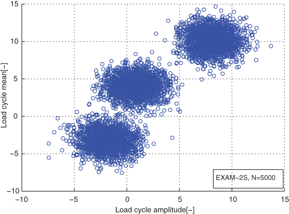
Similarly, the load cycles of the traced vehicles used in the load case EXAM_2S were also generated from a 2D Gaussian mixture distribution. But the mixture Gaussian mixture distribution has three components. The real parameters are as follows: the component numbers K = 3; the weight coefficients π = [0.3 0.3 0.4]; the means of the components µ 1 = [−2 −3], µ 2 = [1 4], µ 3 = [8 10]; the covariance matrix Σ1 = [2 0; 0 3], Σ2 = [2 0; 0 2], Σ3 = [2 0; 0 2]; and the sample size N = 500.
In the load case of EXAM_3S, we used a 2D Gaussian mixture distribution which has five components to generate the load cycles. The real parameters of it are as follows: the component numbers K = 5; the weight coefficients π = [0.2 0.2 0.2 0.2 0.2]; the means of the components µ 1 = [0.5 0.5], µ 2 = [3 2.5], µ 3 = [4 5.5], µ 4 = [5.5 2], µ 5 = [7 5]; the covariance matrix Σ1 = [0.5 0; 0 0.5], Σ2 = [0.4 0; 0 0.3], Σ3 = [0.3 0; 0 0.3], Σ4 = [0.3 0; 0 0.3], Σ5 = [0.5 0; 0 0.5]; and the sample size is the same as other examples N = 500.
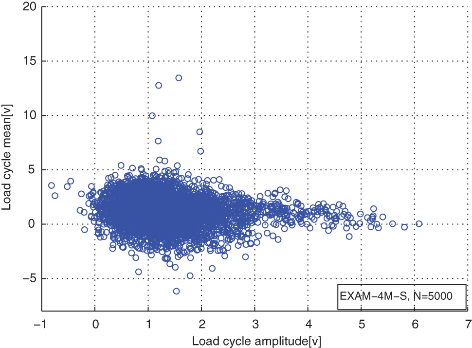
In the measured load case EXAM_4M, the load time series on the loading axis of a certain type of tank was measured under the real operating conditions. The tested tank traveled 100 km on a gravel road with the four gear speed. The load cycles were extracted from a fragment of the whole sample with rainflow counting method. 13 And the units of the load cycle amplitudes and the means are Volts. The number of the measured rainflow load cycles is 2740.
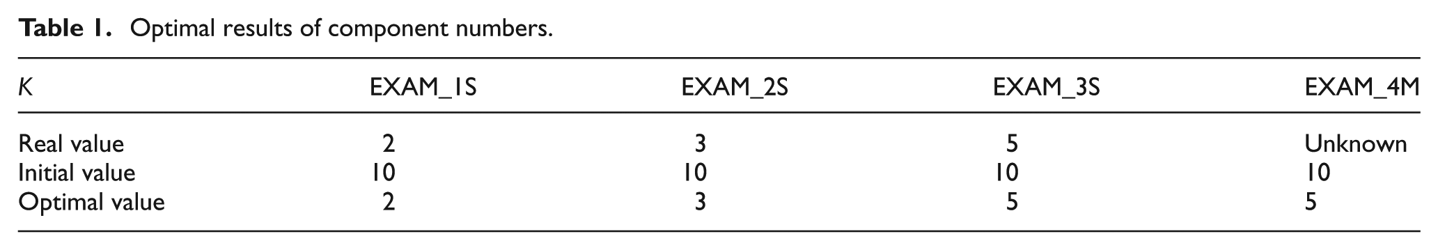
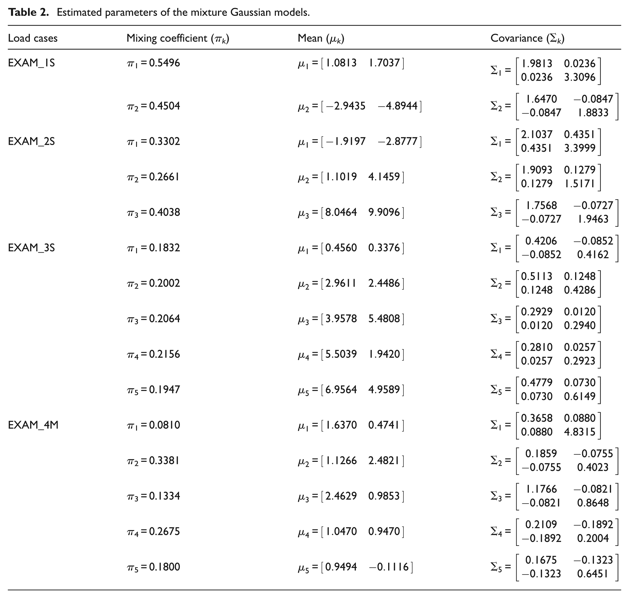
The continuous distributions of rainflow load cycles in those load cases were modeled using a mixture of multivariate Gaussian functions. The rainflow load cycles were represented by a 2D variable denoted by Y = (Ya, Ym ). Ya and Ym represent the means and the amplitudes of the load cycles relatively. The latent variables and parameters were estimated with the variational Bayesian inference method developed in the previous sections. Before the optimal iterations, we have to initialize the prior values of the parameters. In this article, we choose the same prior values for all the load cases. We set α 0 = 0.001, β 0 = 1, m 0 = 0, ν 0 = 20, and w 0 = 200I at the beginning of the iterations. We also set a relatively bigger initial component numbers for the mixture models, K = 10. It was considered convergence when the iteration reaches 2000 steps or the difference of the lower bound value between adjacent iteration steps is less than 1 × 10⁻⁵. After convergence, those components whose weight coefficient is less than 1% × 1/K will be ignored. And they are considered taking essentially no responsibility for the data set. So we can get the optimal value of the component number k. Then, we reset the initial value for K with the estimated result of it and continue the optimal process until the estimated value of K equals the initial value of it. Using this method, we can obtain the final estimated parameters of the mixture Gaussian models. Table 1 shows the optimal results of component numbers of the mixture models for the load cases. The quantitative estimated parameters of the mixture Gaussian models for the load cycle cases are shown in Table 2.
Optimal results of component numbers.
Estimated parameters of the mixture Gaussian models.
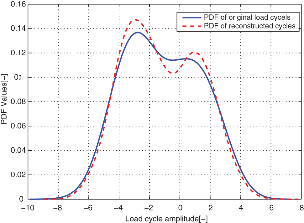
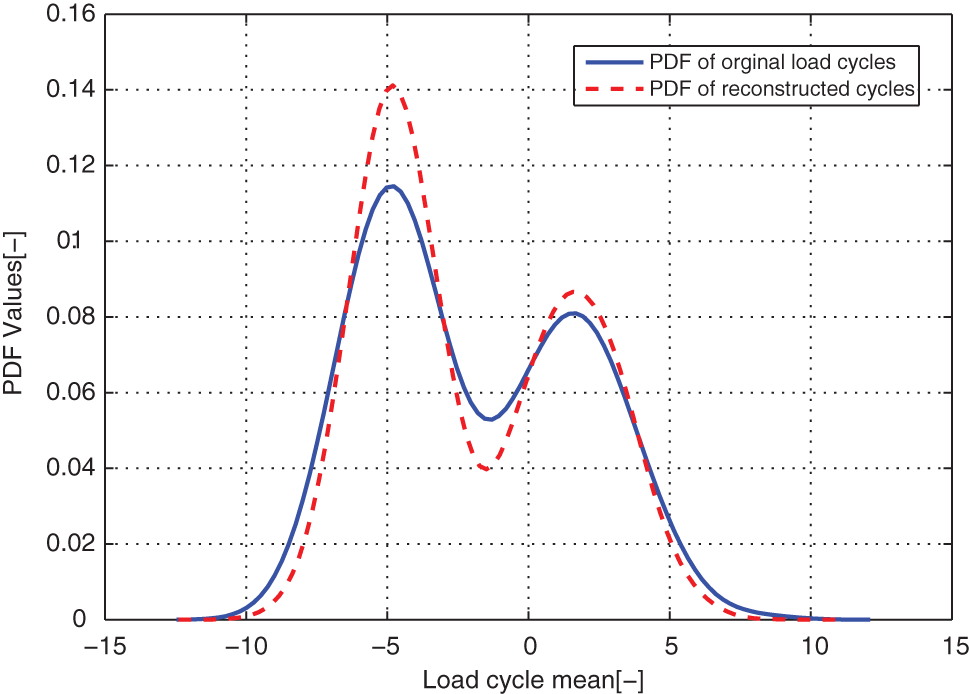
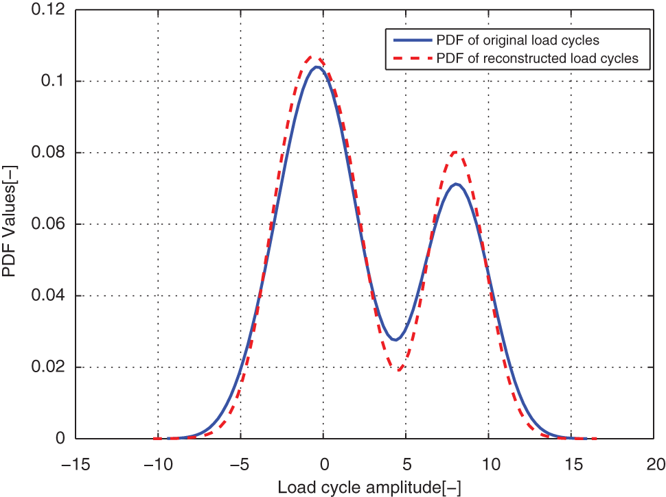
In order to assess the agreement between the original distribution and modeled load spectrum for the load cases, we compared the original load cycle distribution and the reconstructed load cycle distribution. It is difficult to assess the goodness of agreement between modeled PDFs and the original distribution of the rainflow load cycles in 2D space. 6 So we made the comparisons between the modeled one-dimensional (1D) load spectrum with corresponding 1D original marginal PDFs on the load cycle amplitudes and means relatively.
From Table 1, we can see that the agreements between the estimated component numbers and the real component numbers of the mixture models for the simulated load cases are very good. The real component numbers of the mixture model for the measured load case are unknown. And the optimal number of it is 5. The distribution comparisons of the original load cycles and the reconstructed load cycles for the cases of EXAM_1S, EXAM_2S, EXAM_3S, and EXAM_4M are presented in Figures 1–8. Figures 9–16 are the comparisons between the marginal PDFs of original load cycles and marginal PDFs of the reconstructed load cycles on amplitudes and means about the simulated and measured load cases, respectively.
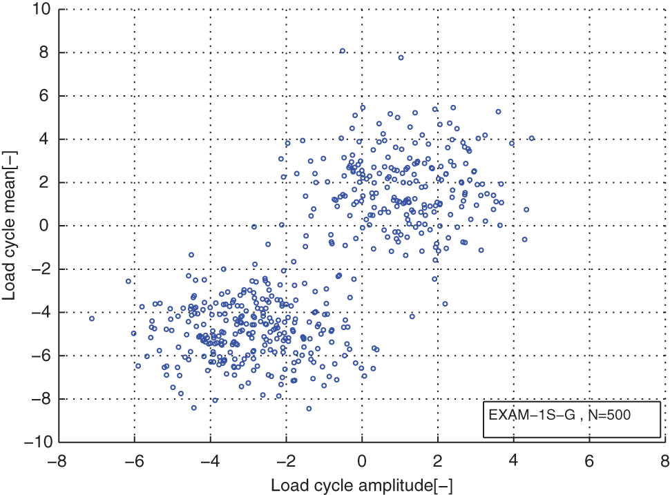
Distribution of the original load cycles for the load case EXAM_1S.
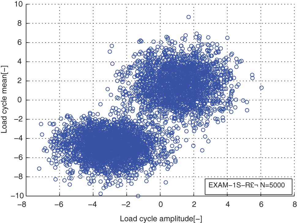
Distribution of the reconstructed load cycles for the load case EXAM_1S.
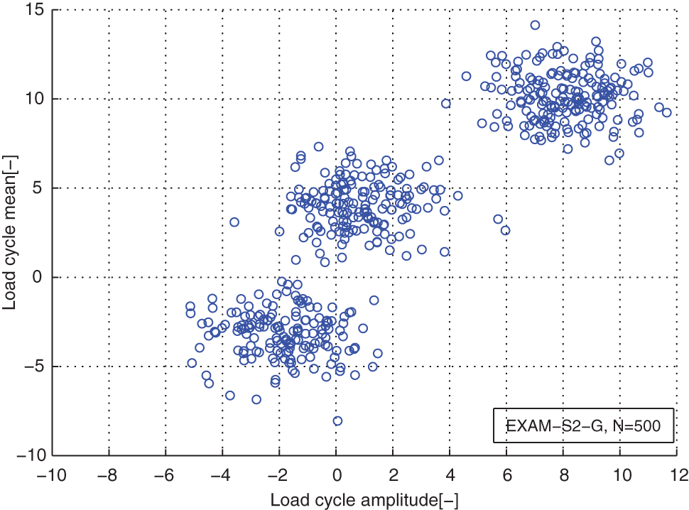
Distribution of the original load cycles for the load case EXAM_2S.
Distribution of the reconstructed load cycles for the load case EXAM_2S.
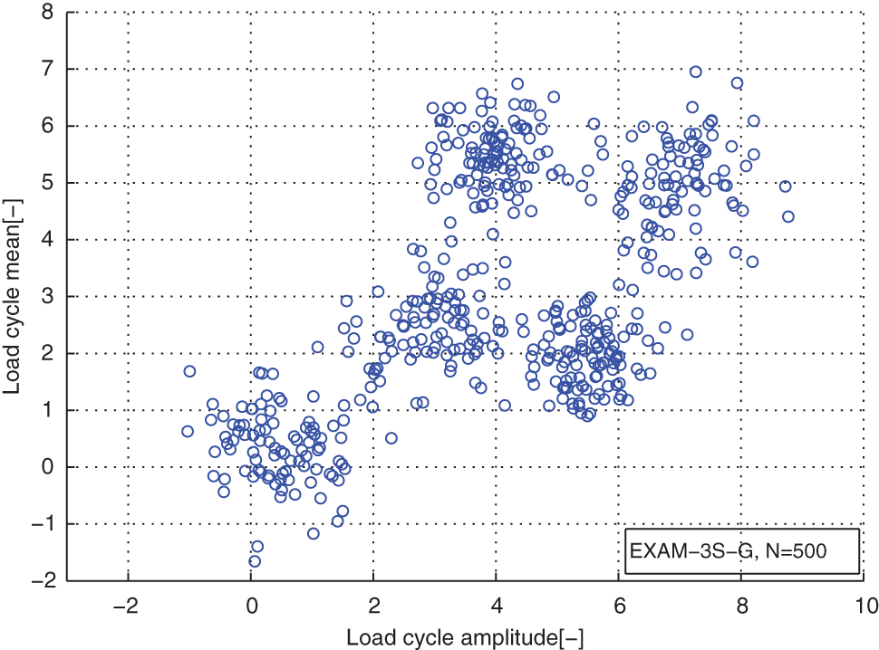
Distribution of the original load cycles for the load case EXAM_3S.
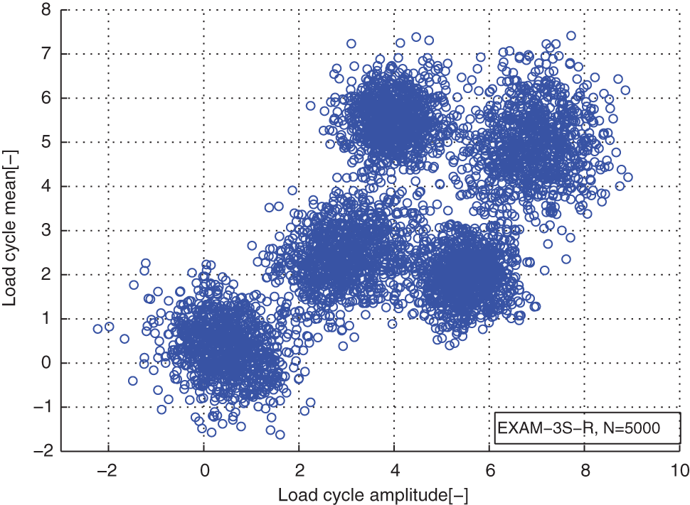
Distribution of the reconstructed load cycles for the load case EXAM_3S.
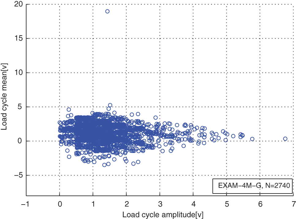
Distribution of the original load cycles for the load case EXAM_4M.
Distribution of the reconstructed load cycles for the load case EXAM_4M.
Comparison of the modeled and original load cycles’ marginal PDF on amplitudes for case EXAM_1S.
Comparison of the modeled and original load cycles’ marginal PDF on means for case EXAM_1S.
Comparison of the modeled and original load cycles’ marginal PDF on amplitudes for case EXAM_2S.
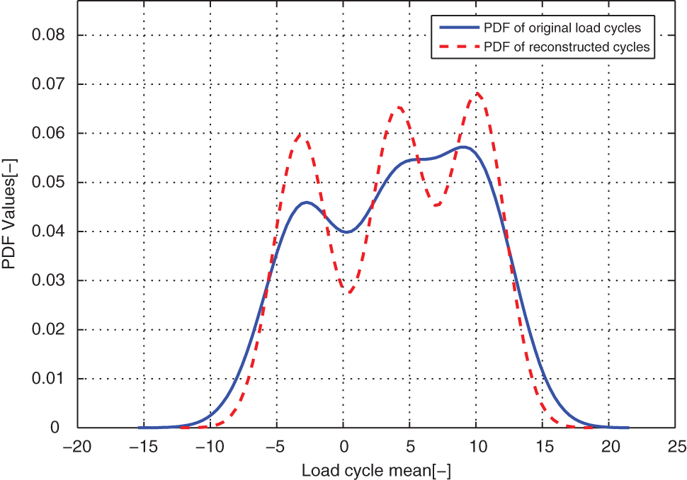
Comparison of the modeled and original load cycles’ marginal PDF on means for case EXAM_2S.
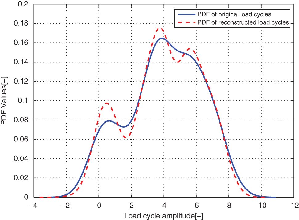
Comparison of the modeled and original load cycles’ marginal PDF on amplitudes for case EXAM_3S.
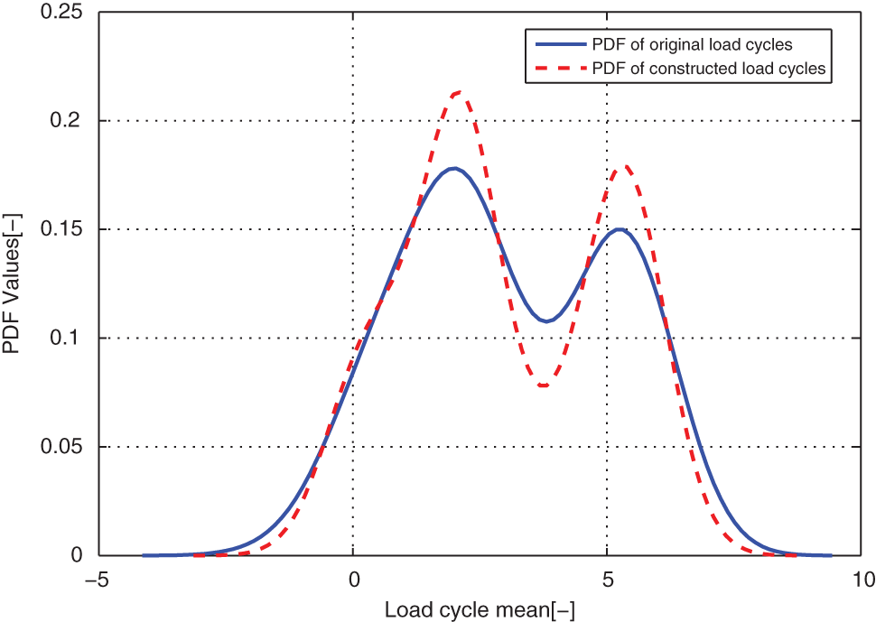
Comparison of the modeled and original load cycles’ marginal PDF on means for case EXAM_3S.
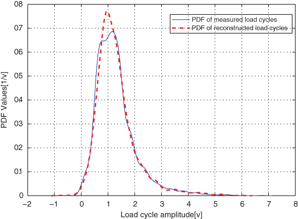
Comparison of the modeled and original load cycles’ marginal PDF on amplitudes for case EXAM_4M.
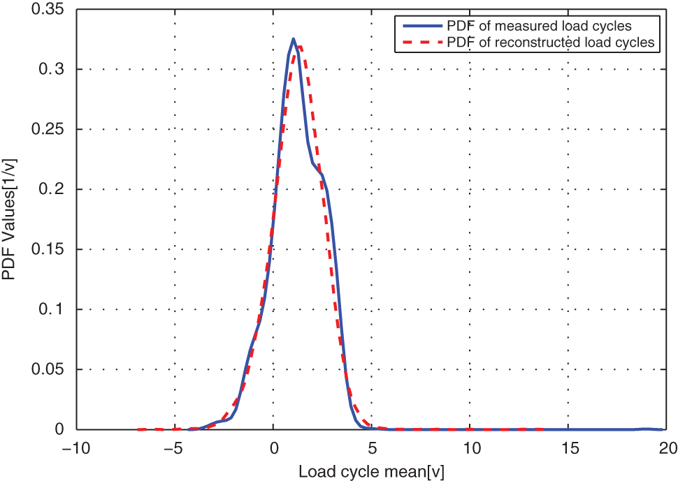
Comparison of the modeled and original load cycles’ marginal PDF on means for case EXAM_4M.
From distribution comparison figures, we can see that the agreements between the original load cycle distributions and the reconstructed load cycle distributions are very well in the shape and distribution density. And the boundaries of those scatters are clear. The marginal PDF figures show that the reconstructed load cycles’ PDF curves have good coincidences with the corresponding ones of original load cycles for all simulated and measured load cases, especially in the regions of low probability. But the reconstructed load cycles’ marginal PDFs tend to that the convex regions are more convex, as well as the concave regions are more concave compared to that of the original load cycles. And it is more evident in the load cases of EXAM_2S and EXAM_3S. This situation may be caused by the estimation error of the means and amplitudes of the Gaussian components of the mixture model. However, from Table 2, we can see that the parameter estimation error of those mixture models is in the acceptable ranges. Thus, the modeled load spectrum for the load cycles agree with the distribution of the original load cycles very well.
Conclusion
In this article, we used the mixture multivariate Gaussian functions to model the load spectrum of tracked vehicles based on rainflow load cycles and presented a parameter estimation method for the mixture distribution model based on variational Bayesian inference. The detailed mathematical procedures were derived when developing the parameter estimation method. Three simulated load cycle cases and one measured load cycle case were used to verify the effectiveness of the load spectrum model and the parameter estimation method. The component numbers can be correctly inferred in all the three simulated load cycle cases given different initial values. Through comparing the marginal PDFs of the original load cycles and the reconstructed load cycles in the cases, the distributions of them agree very well. It was proved that the new algorithm of parameter estimation method can automatically detect the component numbers of the mixture Gaussian model from the observed data set, and it does not depend on the initial conditions. It has good practical value for the engineering applications
Footnotes
Declaration of conflicting interests
The authors declare that there is no conflict of interest.
Funding
This research received no specific grant from any funding agency in the public, commercial, or not-for-profit sectors.