Sage Journals: Discover world-class research

Abstract

Flow stress models in finite element analysis of metal cutting require material parameters that are essential considering the accuracy of the simulations. This article presents a method to acquire material parameters from cutting experiments using the extended Oxley’s shear zone theory. The novelty in this approach is to use measured chip geometry and temperature instead of determining them analytically to calculate strain and strain rate. These values are used to calculate the resultant cutting forces with the extended Oxley’s model and Johnson–Cook flow stress model. Flow stress model parameters are optimized to fit the calculated forces to those measured from cutting experiments. The Johnson–Cook parameters acquired with this method perform better than those found in the literature.

Keywords

Flow stress inverse analysis cutting experiments strain strain rate finite element method AISI 1045

Introduction

Finite element analysis of metal cutting has been established as a research and development method in the field of machining research.¹ The accuracy of the simulations is dependent on the material model used.² In its simplest form, a model approximates the relationship between stress and strain, such as Hooke’s law. The power law equation between stress and strain was used by Oxley³ in his widely referred machining theory. More sophisticated material models include the influence of strain rate and temperature on the stress–strain relationship. One such model is the common Johnson–Cook model.⁴ In addition, damage models add the effect of mechanical and thermal damage to the model which is required, for example, to simulate serrated chip.^5,6 By including elasticity to the simulations, residual stresses can be calculated.⁷ Also, more specific behavior such as yield delay can be taken into account.⁸

One general outcome in the research articles is that the modeling of the stress–strain behavior itself is not the problem, but rather the determination of the material parameters for each model.⁹ Determination of the material parameters for a model is difficult because testing conditions do not match the real cutting conditions. For example, during a compression test, the material is under a much slower strain rate and a lower temperature than during machining. The contact conditions in cutting are more or less unique, so by acquiring the material parameters by means of materials testing much of the relevant data are left out. To avoid the above-mentioned difficulties, few improvements in testing have been made. To gain flow stress at a high deformation rate, split Hopkinson’s pressure bar (SHPB) testing is used.¹⁰ Nevertheless, the strain rate and in some cases the temperature are too low compared to cutting conditions. Strain rate values as high as 20,000 s⁻¹ can be achieved by SHPB testing, whereas cutting involves strain rates up to 10⁶ s⁻¹. By using a preheated test specimen, SHPB testing can be done in temperatures as high as 900 °C which is high enough for most materials. The most common approach is to compile the material parameters from data gathered from materials testing and orthogonal cutting tests.¹¹ Apart from the cutting forces, different phenomena occurring during cutting are difficult to measure because of high speeds and loads. For that, determining the real stress–strain relationship of a material based only on direct measurement is complicated. Even though it is difficult to measure flow stress or hardening effects from cutting tests, they are the most reliable source of acquiring material parameters. Therefore, inverse analysis with simulations or analytical models is often used. Inverse analysis with simulations means running the simulations and using a full-factorial analysis on each parameter or optimizing the results parameter by parameter deductively.^12,13 Inverse analysis with analytical model means calculating theoretical values of strain, strain rate and flow stress from measurable factors such as cutting forces, chip thickness and shear angle to obtain parameters for material models by fitting the model curve to the measured values.¹⁴ The most used analytical model is the parallel sided shear zone model, often referred to as Oxley’s model, which has been developed in parts by Piispanen,¹⁵ Eugene Merchant¹⁶ and Oxley,³ among others.

Parallel sided shear zone theory

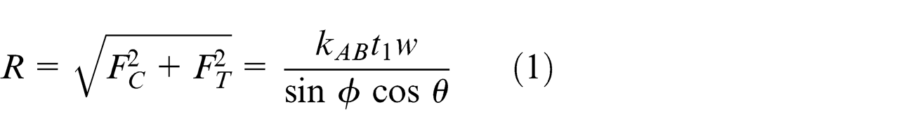
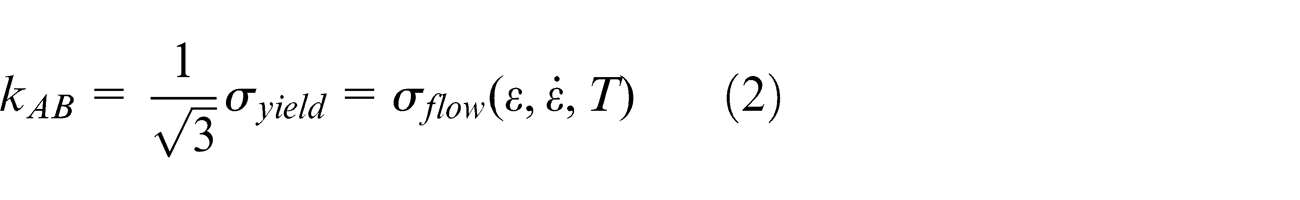
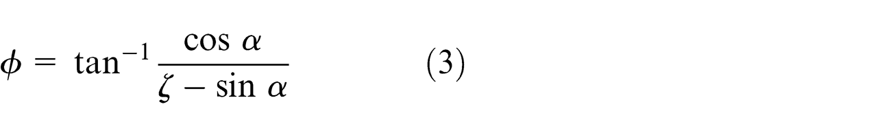
The orthogonal cutting model proposed by Oxley is based on a model where deformation of the material takes place in a parallel sided zone that follows the shear angle. The geometrical definition of the model is presented in Figure 1, and equations (1)–(8) present the relevant model details.³ Boothroyd and Knight¹⁷ have developed a temperature prediction model presented in equations (9)–(12)). Lalwani et al.¹⁸ proposed an extension that enables Oxley’s model to be used with other than the Power law material model. 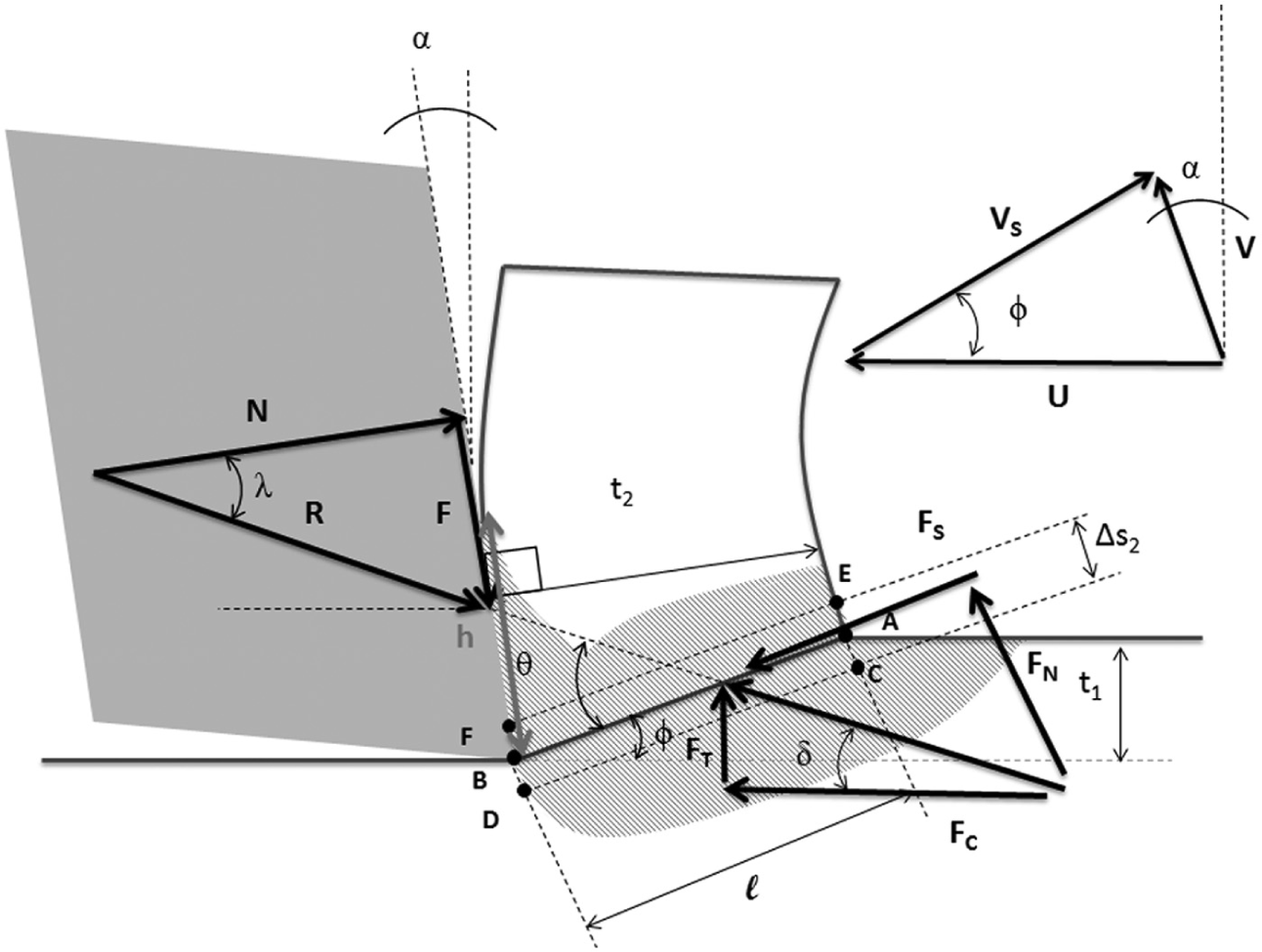The strain hardening exponent $n$ and strain rate constant $C_{0}$ require modifications, which are presented in equations (13) and (14) for the Johnson–Cook model.

Figure 1.

Parallel sided shear zone model.

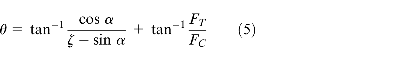
Resultant force¹⁹

R = \sqrt{F_{C}^{2} + F_{T}^{2}} = \frac{k_{AB} t_{1} w}{\sin ϕ \cos θ}

(1)

Specific cutting force³

k_{AB} = \frac{1}{\sqrt{3}} σ_{yield} = σ_{flow} (ε, \overset{\cdot}{ε}, T)

(2)

Shear angle¹⁶

ϕ = \tan^{- 1} \frac{\cos α}{ζ - \sin α}

(3)

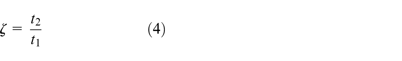
Chip compression ratio (CCR)²⁰

ζ = \frac{t_{2}}{t_{1}}

(4)

Oxley’s model³

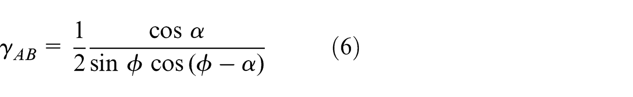
θ = \tan^{- 1} \frac{\cos α}{ζ - \sin α} + \tan^{- 1} \frac{F_{T}}{F_{C}}

(5)

Shear strain¹⁶

γ_{AB} = \frac{1}{2} \frac{\cos α}{\sin ϕ \cos (ϕ - α)}

(6)

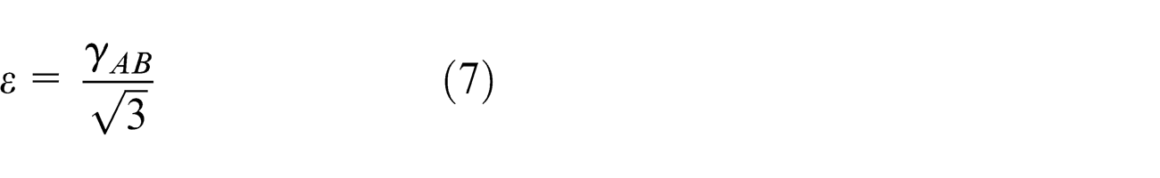
Equivalent strain³

ε = \frac{γ_{AB}}{\sqrt{3}}

(7)

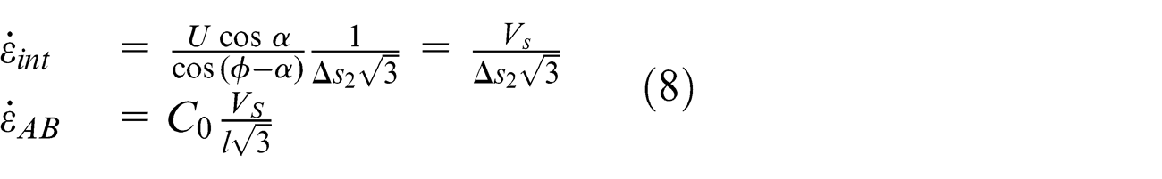
Strain rates in tool–chip interface and shear sone³

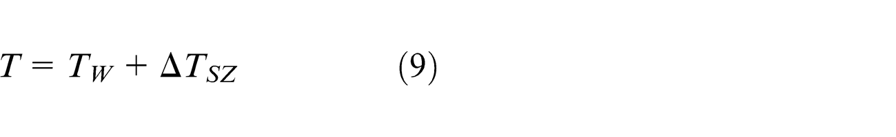
\begin{matrix} {\overset{\cdot}{ε}}_{int} & = \frac{U \cos α}{\cos (ϕ - α)} \frac{1}{Δ s_{2} \sqrt{3}} = \frac{V_{s}}{Δ s_{2} \sqrt{3}} \\ {\overset{\cdot}{ε}}_{AB} & = C_{0} \frac{V_{S}}{l \sqrt{3}} \end{matrix}

(8)

Shear zone temperature¹⁷

T = T_{W} + Δ T_{SZ}

(9)

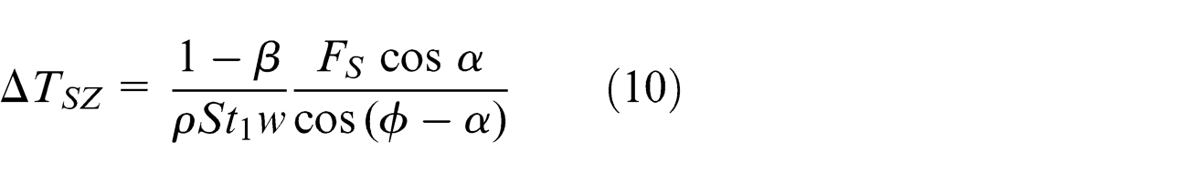
Temperature rise in shear zone¹⁷

Δ T_{SZ} = \frac{1 - β}{ρ {St}_{1} w} \frac{F_{S} \cos α}{\cos (ϕ - α)}

(10)

Proportion of heat conducted to workpiece¹⁷

β = a_{%} + b_{%} \log (R_{T} \tan ϕ)

(11)

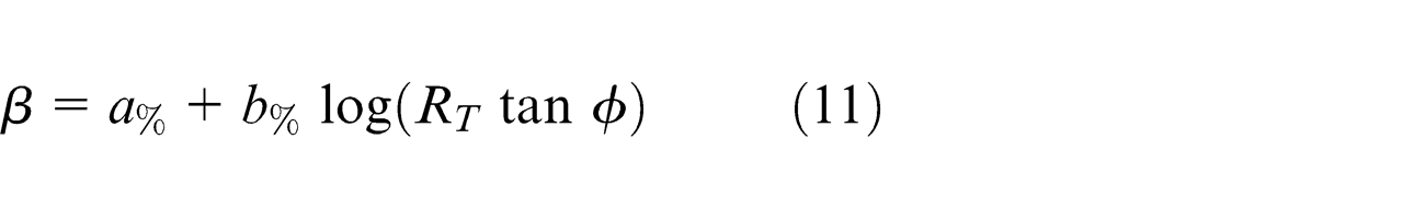
Dimensionless thermal number¹⁷

\begin{matrix} R_{T} = \frac{ρ {SUt}_{1}}{K} \\ R_{T} \tan ϕ ⩽ 10 \\ a_{%} = 0.5 b_{%} = - 0.35 \\ R_{T} \tan ϕ > 10 \\ a_{%} = 0.3 b_{%} = - 0.15 \end{matrix}

(12)

Mod. strain hardening exponent¹⁸

n_{eq} = \frac{d σ_{AB}}{d ε_{AB}} (\frac{ε_{AB}}{σ_{AB}}) = \frac{nB ε_{AB}^{n}}{(A + B ε_{AB}^{n})}

(13)

Mod. strain rate constant¹⁸

C_{0} = 1 + 2 (\frac{π}{4} - ϕ) - \frac{\tan θ}{n_{eq}}

(14)

Different measures of strain and strain rate

In this article, three measures of strain are investigated, which are proposed by Oxley, Merchant and Astakhov. Strain proposed by Oxley is presented in equation (6). Merchant’s strain is presented in equation (15) and Astakhov’s and Shvets’²¹ strain is presented in equation (16). All strains can be expressed in terms of shear angle and rake angle, or rake angle and CCR. One noteworthy observation is that Oxley’s strain is exactly the same as Merchant’s strain, but it is divided by $2 \sqrt{3}$ , and there is a geometrical explanation for this in equation (17). Oxley’s strain is divided by 2 because it is assumed that half of the deformation has taken place when the material reaches the AB-line and $\sqrt{3}$ comes from von Mises’ equivalent strain definition. Strains are plotted in Figure 2 with a rake angle range of ±20°. Oxley’s and Astakhov’s strains are closer to each other since they represent an equivalent strain in a major shear zone, whereas Merchant’s strain is a presentation of the total strain in a chip formation zone. Astakhov and Shvets²¹ argue that Merchant’s presentation of strain is invalid because when the CCR is 1, there is no geometrical deformation, so the strain should be 0 at this point, which is not the case with Merchant’s model. Figure 3 shows the strain plotted against CCR, which shows Astakhov’s argument about a non-zero strain at a CCR value of 1. Merchant’s definition of strain and strain rate is evaluated in Davim and Maranhão²² using simulations. Finite element method (FEM) results support Merchant’s model, but the article unfortunately does not provide simulated temperatures or cutting forces to evaluate the accuracy of the simulations. For extended Oxley’s model to produce results that are aligned with the theory, the original Oxley’s definition of strain should be used. Otherwise the flow stress is overestimated by a magnitude of 100%−200%.

Figure 2.

Different strains plotted against shear angle with rake angles of ±20°.

Figure 3.

Different strains plotted against CCR with rake angles of ±20°.

Merchant’s strain

ε = \cot (ϕ) + \tan (ϕ - α)

(15)

Astakhov’s strain

ε = 1.15 \ln ζ

(16)

Geometrical explanation

ζ = \frac{\cos α}{\tan ϕ} + \sin α = \frac{\cos (ϕ - α)}{\sin ϕ}

(17)

Flow stress models

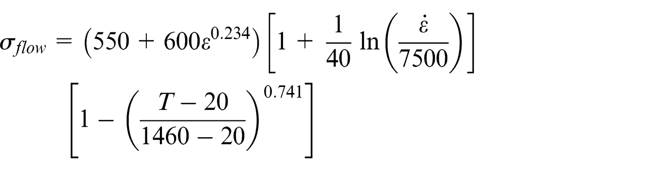
Flow stress is normally presented as a function of strain, strain rate and temperature, although the form of the function varies. The Johnson–Cook model⁴ (equation (18)) is formulated for materials under high strain rate and is one of the most used models in the field of metal cutting. The most common flow stress models used in cutting simulations are presented in Appendix 2, equations (19)–(24). Zerilli and Armstrong model²³ (equation (23)) is special since it has different equations for BCC and FCC materials. Another unusual model is Maekawa’s model because of strain path dependency.²⁴

Research objectives

In order to take advantage of cutting simulations in academia or industry, material modeling must be efficient time and cost vice. This research article investigates a robust method of acquiring material model parameters directly from cutting experiments. If this method performs as expected, the material parameter acquisition will be more efficient than with high-speed compression tests. The results show whether analytical models are viable option to be used in an inverse analysis routine and whether further development of the method is advisable. The results are evaluated in the framework of previous studies on the same material.

Challenges in experimental setup

Forces, chip thicknesses and cutting parameters are easy to obtain reliably from cutting experiments, but temperatures, actual strain and strain rate are difficult to measure. Approaches with thermal couple, thermal sensors and pyrometers or infrared (IR) imaging have been tried with a variety of results.^25–29 A thermal couple measures the largest temperature difference between a tool and a workpiece; thermal sensors and pyrometers can be set to measure the surface temperatures of a newly machined layer or a tool. Thermal imaging can measure anything in theory, but practicalities such as imaging frame rate and different emissivity of surfaces cause challenges. Strain and strain rate can be measured using analytical models, quick stop experiments with metallography or digital image correlation during machining.³⁰ Analytical models are only accurate in an orthogonal cutting setup and only for some materials and cutting parameters. Quick stop experiments provide reliable results but are slow and expensive to conduct and the quick stop device or setup is never infinitely fast so the obtained sample does not fully represent the actual cutting condition. Digital image correlation is a promising method, but frame rate and optics resolution need to be improved to measure strain and strain rate in real cutting speeds (>100 m/min).³⁰

Experimental inverse analysis routine

In this article, an inverse analysis routine is formulated to acquire Johnson–Cook parameters from cutting experiments. This approach is different from that presented by Sartkulvanich et al.¹⁴ since in their OXCUT model inputs are cutting conditions and material properties but no experimentally determined strain, strain rate and temperature values. The novelty in this approach is to use experimental values for chip thickness and temperature to avoid error caused by the analytical model. Chip geometry and temperature are measured from cutting experiments. Chip thickness is measured and CCR is calculated with equation (4). Rake angle together with CCR give shear zone angle with equation (3). Next, the strain and strain rate are calculated from chip geometry using definitions from the parallel sided shear zone theory. Then, using these values of the strain, strain rate and temperature instead of those determined from the analytical model, the extended Oxley’s model is used to calculate cutting forces. These cutting force values are compared to the experimental values of AISI 1045 that can be found in the literature. Using the obtained data set, a flow stress model (Johnson–Cook) is calibrated by optimizing the parameters of the model to fit it to the obtained flow stress–strain–strain rate–temperature data set. The results are compared to other Johnson–Cook parameter sets found from the literature.

Materials and methods

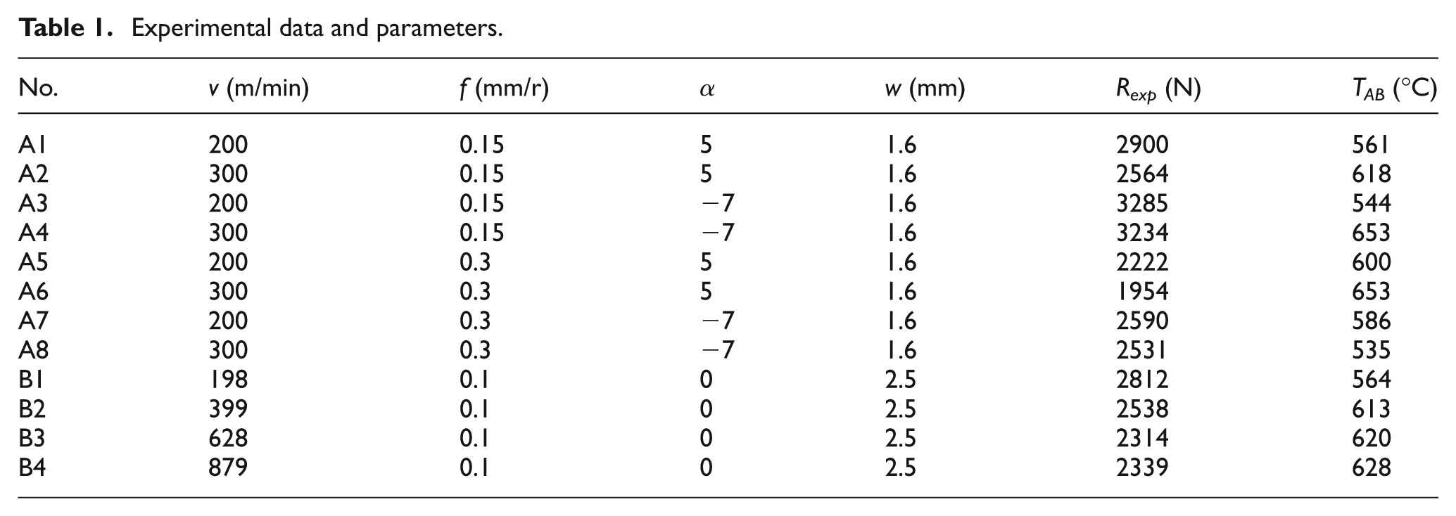
The inverse analysis routine is based on extended Oxley’s model with Johnson–Cook flow stress model. Flowchart of the whole routine is presented in Figure 4. The resultant cutting force is calculated with equation (1). For this, flow stress and chip geometry are needed. Flow stress is calculated from the flow stress model, which needs strain, strain rate and temperature as input parameters. The strain and strain rate are calculated from the chip geometry with Oxley’s model equations (7) and (8). Input parameters for the model are cutting speed, feed, width and rake angle. Also, experimentally obtained values of chip thickness, shear zone angle and temperature are used as input parameters. The predicted resultant forces are evaluated against experimentally obtained values, and flow stress model parameters are adjusted for a better fit until the optimal solution. The optimization routine minimized the error of the normalized resultant cutting forces with the least squares method. Experiment data and parameters are presented in Table 1. The resultant force is calculated as the root of the sum of squares of each force component. Experimental data for the cutting of AISI 1045 are acquired from literature sources: A1–A8 from Ivester et al. and B1–B4 from Iqbal et al.^31–34 and Ivester et al. used orthogonal turning for their tests. The tool used was a Kennametal K68, an uncoated general-purpose tungsten carbide insert with rake angles of +5° and −7°. Cutting forces were measured with a Kistler 9257B 3-component piezoelectric dynamometer and 9403 mount. Cutting temperatures were measured with an intrinsic thermocouple and selected experiments with IR-microscopy. The experiments were conducted twice for each cutting parameter set in four different laboratories to ensure repeatability. Resultant forces from Ivester et al. are average of all the experiments except clearly anomalous results were discarded from the average. Iqbal et al. conducted similar experiments with a lathe and a Kistler 9263A dynamometer using uncoated Sandvik TCMW 16T304 grade 5015 inserts. The article does not report how many repetitions were conducted so it is assumed that no repetitions have been done. Experimental data by Ivester have been used as well in Lalwani et al.¹⁸ and Ding and Shin,³⁵ but the temperature values used in these articles are for some reason twice as high as those in Ivester’s articles. The original values presented by Ivester are used in this article. This decision is encouraged by the temperature results in Davies et al.²⁶ and their thermal imaging experiments, where the results are similar to those in Ivester et al. Temperatures for experiments B1–B4 are determined from the simulations of Ding and Shin and considering Ivester’s results because Iqbal et al. did not present any temperature measurements for their experiments.

Figure 4.

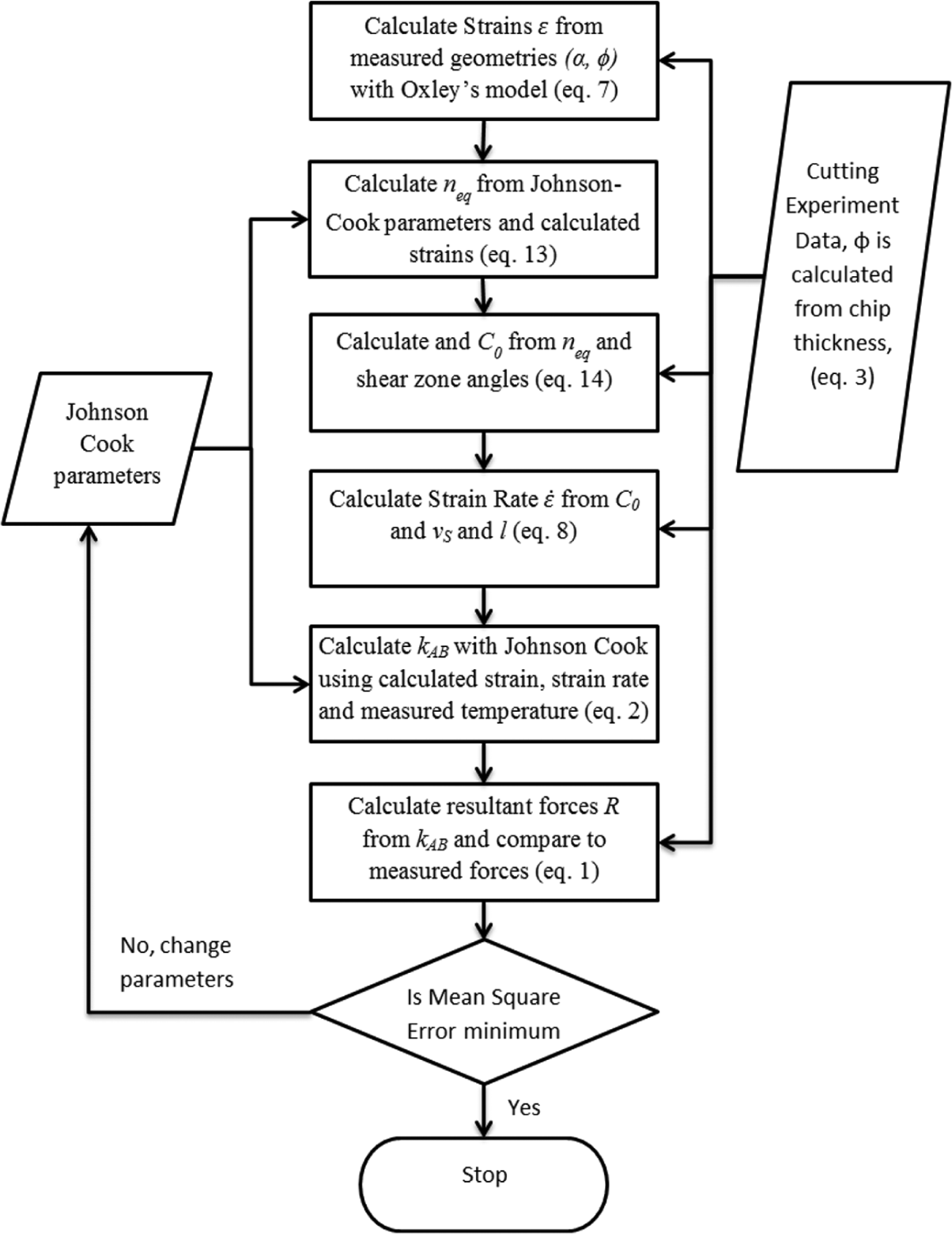
Inverse analysis routine flowchart.

Table 1.

Experimental data and parameters.

No.	v (m/min)	f (mm/r)	α	w (mm)	R_exp (N)	T_AB (°C)
A1	200	0.15	5	1.6	2900	561
A2	300	0.15	5	1.6	2564	618
A3	200	0.15	−7	1.6	3285	544
A4	300	0.15	−7	1.6	3234	653
A5	200	0.3	5	1.6	2222	600
A6	300	0.3	5	1.6	1954	653
A7	200	0.3	−7	1.6	2590	586
A8	300	0.3	−7	1.6	2531	535
B1	198	0.1	0	2.5	2812	564
B2	399	0.1	0	2.5	2538	613
B3	628	0.1	0	2.5	2314	620
B4	879	0.1	0	2.5	2339	628

Johnson–Cook model parameters for AISI 1045

The Johnson–Cook model includes strain hardening parameters $A, B, n$ and rate hardening parameter $C$ and thermal softening parameter $m$ . The Johnson–Cook parameter sets acquired from inverse analysis and the literature are presented in Table 2. The errors in Table 2 are calculated as average, minimum and maximum of the percentile errors for each individual cutting condition between average resultant forces acquired from experiments and analytical method. The experimental values used are the average of each parameter’s set. Sets 1–3 are from inverse analysis. Set 1 was optimized by varying only $C$ and $m$ , set 2 was optimized by varying all parameters with the reference strain rate at 7500 s⁻¹ and set 3 was similarly optimized with the reference strain rate at 0.001 s⁻¹. Parameter A is bounded between 290 and 660 MPa because A represents yield stress in the model. Other variables are bounded between [0; 10] except B, which is between [0; 1000]. Set 4 is from Lalwani et al.¹⁸ and set 5 is from Klocke et al.¹² Lalwani et al. used the Johnson–Cook parameters found in Jaspers and Dautzenberg³⁶ and the experimental results of Ivester. Jaspers et al. used SHPB experiments to determine their values. Lalwani et al. did not perform any inverse analysis in their work. Buchkremer et al. used the Johnson–Cook parameters A, B and n from Abouridouane et al.³⁷ and for C and m they performed a full-factorial analysis, basically running simulations of all combinations of the factors. The cutting experiments were done at RWTH Aachen University with a Broaching Machine, a Kistler dynamometer and a two-color pyrometer. The cutting experiment data set is with feed 0.1–0.4 and 50 and 100 m/min for cutting speed.

Table 2.

Johnson–Cook parameters from different sources and accompanying errors.

No.	1	2	3	4	5
A	550	391	290	553	546
B	600	217	283	601	487
n	0.234	0.340	0.249	0.234	0.250
C	0.025	0.003	0.004	0.013	0.027
m	0.741	3.283	3.365	1.000	0.631
T_melt	1460	1460	1460	1460	1460
T_ref	20	20	20	20	20
(dε/dt)_ref	7500	7500	0.001	7500	0.001
Average (%)	5.3	5.0	5.0	20.4	13.4
Maximum (%)	12.6	9.9	9.9	34.9	28.4
Minimum (%)	0.0	1.1	1.1	7.5	0.8
ΣE²	0.06	0.04	0.04	0.57	0.29

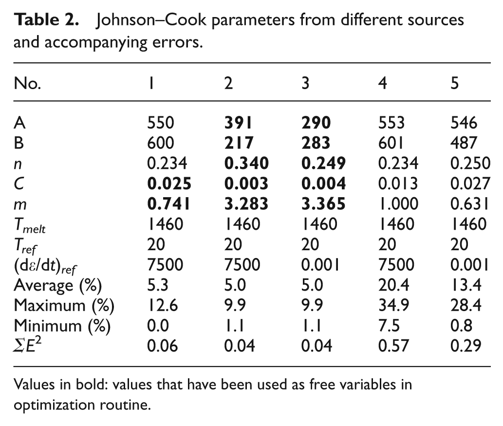
Values in bold: values that have been used as free variables in optimization routine.

Results and discussion

Using the proposed method, an average error of less than 6% is achieved, whereas parameters obtained from the literature produce an average error of 20% and 13%. All parameters are relatively of the same magnitude with the greatest variation in the values of $C$ and $m$ . Figure 5 presents the normalized resultant forces from experiments and predicted values using all four different flow stress parameter sets. Sets 1–3 follow experimental results well. Sets 2 and 3 estimate the effect of rate sensitivity lower and thermal softening higher than sets 1, 4 and 5. A noteworthy point is that the data are from multiple sources and from a wide cutting parameter scope (e.g. a cutting speed from 200 to 870 m/min), but despite that the model follows the data well. One point to consider is the uniqueness of the solutions since parameter sets 1–3 produce results that are very close to each other, but the parameters are clearly different. It could be that cutting has too fuzzy mechanistic properties for cutting experiments to clearly differentiate hardening mechanisms from each other. For example, an increase in cutting speed leads to an increase in strain rate and temperature, and the cause of the proportional increase in the resultant force in this case cannot be determined unambiguously. This was also implied by a graph analysis of metal cutting parameters in Laakso et al.³⁸ A linear relationship between strain, strain rate or temperature and machining parameters cannot be formed. Therefore, the role of compression experiments or SHPB experiments could be irreplaceable, because in these experiments, one variable can be changed while other variables are controlled.

Figure 5.

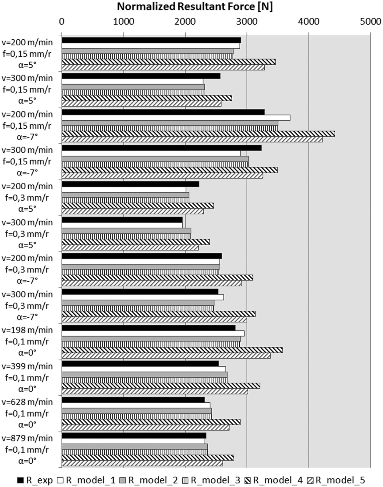
Comparison of experimental resultant forces with modeled resultant forces.

Conclusion

In this article, an inverse analysis of flow stress model parameters was conducted to optimize the model performance. The following important points were observed:

The method produces better performing flow stress model parameter values for an analytical model than those found in the literature

\begin{matrix} σ_{flow} = (550 + 600 ε^{0.234}) [1 + \frac{1}{40} \ln (\frac{\overset{\cdot}{ε}}{7500})] \\ [1 - {(\frac{T - 20}{1460 - 20})}^{0.741}] \end{matrix}

A clear relationship between flow stress model variables and cutting parameters is difficult to form; therefore, a wide range of cutting parameters should be used.

There are many local optimal solutions for flow stress model parameters. Therefore, it is advisable to use compression test values for setting the reference frame for the model parameters.

The method is promising and further study is required to identify more delicate material behavior related to thermal effects.

Footnotes

Appendix 1

Appendix 2 Declaration of conflicting interests

The authors declare that there is no conflict of interest.

Funding

This research received no specific grant from any funding agency in the public, commercial, or not-for-profit sectors.

References

Marusich

Ortiz

. Modeling and simulation of high speed machining. Int J Numer Meth Eng 1995; 38(21): 3675–3694.

Laakso

SVA

. Finite element modeling of cutting—applications and usability. Master’s Thesis, Helsinki University of Technology, Helsinki, 2009 (in Finnish).

Oxley

PLB

. The mechanics of machining: an analytical approach to assessing machinability (Ellis Horwood series in mechanical engineering). West Sussex, UK: Market Cross House, 1989.

Johnson

Cook

. A constitutive model and data for metals subjected to large strains, high strain rates and high temperatures. In: Proceedings of the 7th international symposium on ballistics, The Hague, 19–21 April 1983, vol. 21, pp.541–547. Hague, Netherlands: International Symposium on Ballistics, American Defense Preparedness Association, and Koninklijk Instituut van Ingenieurs.

Pantalé

Bacaria

Dalverny

. 2D and 3D numerical models of metal cutting with damage effects. Comput Method Appl M 2004; 193(39): 4383–4399.

Guo

Yen

. A FEM study on mechanisms of discontinuous chip formation in hard machining. J Mater Process Tech 2004; 155–156: 1350–1356.

Marusich

Askari

. Modeling residual stress and workpiece quality in machined surfaces. In: Proceedings of the fourth CIRP international workshop modeling of machining operations, Delft Technological University, Delft, 17–18 August 2001, pp.105–109.

Childs

THC

. Modelling orthogonal machining of carbon steels. Part I: strain hardening and yield delay effects. Int J Mech Sci 2009; 51(5): 402–411.

Sartkulvanich

. Determination of material properties for use in FEM simulations of machining and roller burnishing. PhD Dissertation, Ohio State University, Columbus, OH, 2007.

10.

Apostol

Vuoristo

Kuokkala

. High temperature high strain rate testing with a compressive SHPB. J Phys IV 2003; 110: 459–464.

11.

Laakso

SVA

Hokka

Niemi

. Investigation of the effect of different cutting parameters on chip formation of low-lead brass with experiments and simulations. Proc IMechE, Part B: J Engineering Manufacture 2013; 227(11): 1620–1634.

12.

Klocke

Lung

Buchkremer

. Inverse identification of the constitutive equation of Inconel 718 and AISI 1045 from FE machining simulations. Proced CIRP 2013; 8: 212–217.

13.

Sartkulvanich

Lopez

Rodriguez

. Inverse analysis methodology to determine flow stress data for finite element modeling of machining. In: 11th CIRP conference on modeling of machining operation, Gaithersburg, MD, 16–18 September 2008, http://nsm.eng.ohio-state.edu/CIRPNIST_paper_inverse_machining_2008.pdf (accessed 15 April 2014).

14.

Sartkulvanich

Koppka

Altan

. Determination of flow stress for metal cutting simulation—a progress report. J Mater Process Tech 2004; 146(1): 61–71.

15.

Piispanen

. Theory of formation of metal chips. J Appl Phys 1948; 19: 876–881, http://dx.doi.org/10.1063/1.1697893

16.

Eugene Merchant

. Mechanics of the metal cutting process. I. Orthogonal cutting and a type 2 chip. J Appl Phys 1945; 16: 267–275, http://dx.doi.org/10.1063/1.1707586

17.

Boothroyd

Knight

. Fundamentals of machining and machine tools. 2nd ed. New York: Marcel Dekker, Inc., 1989.

18.

Lalwani

Mehta

Jain

. Extension of Oxley’s predictive machining theory for Johnson and Cook flow stress model. J Mater Process Tech 2009; 209(12–13): 5305–5312.

19.

Taylor

. On the art of cutting metals. New York: Transactions of ASME, 1907.

20.

Zorev

. Metal cutting mechanics. Oxford: Pergamon Press, 1966.

21.

Astakhov

Shvets

. The assessment of plastic deformation in metal cutting. J Mater Process Tech 2004; 146(2): 193–202.

22.

Davim

Maranhão

. A study of plastic strain and plastic strain rate in machining of steel AISI 1045 using FEM analysis. Mater Design 2009; 30(1): 160–165.

23.

Zerilli

Armstrong

. Dislocation mechanics based constitutive relations for materials dynamics calculations. J Appl Phys 1987; 61(6): 1816–1825.

24.

Maekawa

Shirakashi

Usui

. Flow stress of low carbon steel at high temperature and strain rate (part 2)—flow stress under variable temperature and variable strain rate. B Jpn Soc Prec Eng 1983; 17(3): 167–172.

25.

Abhang

Hameedullah

. Chip-tool interface temperature prediction model for turning process. Int J Eng Sci Tech 2010; 2(4): 382–393.

26.

Davies

Cooke

Larsen

. High bandwidth thermal microscopy of machining AISI 1045 steel. CIRP Ann: Manuf Techn 2005; 54(1): 63–66.

27.

Heisel

Storchak

Eberhard

. Experimental studies for verification of thermal effects in cutting. Prod Engineer 2011; 5(5): 507–515.

28.

Longbottom

Lanham

. Cutting temperature measurement while machining—a review. Aircr Eng Aerosp Tec 2005; 77(2): 122–130.

29.

Artozoul

Lescalier

Bomont

. Extended infrared thermography applied to orthogonal cutting: mechanical and thermal aspects. Appl Therm Eng 2014; 64: 441–452.

30.

Mahadevan

. Experimental determination of velocity and strain rate fields in metal cutting of OFHC copper. Master’s Thesis, Wichita State University, 2007, http://soar.wichita.edu/handle/10057/1522 (accessed 15 April 2014).

31.

Ivester

Kennedy

Davies

. Assessment of machining models: progress report. Mach Sci Technol 2000; 4(3): 511–538.

32.

Ivester

Kennedy

. Comparison of machining simulations for 1045 steel to experimental measurements. SME paper TPO4PUB336, 2004, pp.1–15.

33.

Iqbal

Mativenga

Sheikh

. Characterization of machining of AISI 1045 steel over a wide range of cutting speeds. Part 1: investigation of contact phenomena. Proc IMechE, Part B: J Engineering Manufacture 2007; 221(5): 909–916.

34.

Iqbal

Mativenga

Sheikh

. Characterization of machining of AISI 1045 steel over a wide range of cutting speeds. Part 2: evaluation of flow stress models and interface friction distribution schemes. Proc IMechE, Part B: J Engineering Manufacture 2007; 221(5): 917–926.

35.

Ding

Shin

. A metallo-thermomechanically coupled analysis of orthogonal cutting of AISI 1045 steel. J Manuf Sci E: T ASME 2012; 134(5): 051014.

36.

Jaspers

SPFC

Dautzenberg

. Material behaviour in conditions similar to metal cutting: flow stress in the primary shear zone. J Mater Process Tech 2002; 122(2–3): 322–330.

37.

Abouridouane

Klocke

Lung

. A new 3D multiphase FE model for micro cutting ferritic–pearlitic carbon steels. CIRP Ann: Manuf Techn 2012; 61(1): 71–74.

38.

Laakso

SVA

Peltokorpi

Ratava

. Graph-based analysis of metal cutting parameters. In: Azevedo

(ed.) Advances in sustainable and competitive manufacturing systems (Lecture Notes in Mechanical Engineering). Berlin: Springer, 2013, pp.627–636.

Determination of material model parameters from orthogonal cutting experiments

Abstract

Keywords

Introduction

Parallel sided shear zone theory

Different measures of strain and strain rate

Flow stress models

Research objectives

Challenges in experimental setup

Experimental inverse analysis routine

Materials and methods

Johnson–Cook model parameters for AISI 1045

Results and discussion

Conclusion

Footnotes

Appendix 1

Appendix 2

Declaration of conflicting interests

Funding

References