
Abstract
In a machining process, the workpiece is usually machined by several passes to achieve the desired dimension and form. Workpiece deviation generated in the previous pass will affect the next pass. A new point-based variation propagation model for a single machining process with multi-passes was proposed in this article to investigate the relationships between different passes. The effects of locating errors, geometric errors of machine tool, and tool deflection on workpiece deviation are analyzed. Based on these analyses, a point-based variation propagation model for a machining process with multi-passes was derived. By including the influence of the tool deflection, a linkage between workpiece deviation and the cutting parameters is established. Since different passes are distinguished by their cutting parameters, the relationships between different passes are built up via this model. At the end of this article, case studies were carried out to validate the model and its application in cutting parameters’ optimization.
Introduction
The performance and quality of mechanical products are mainly determined by the machining process. The materials are moved from the workpiece in a machining process to acquire a higher accuracy and more complicated surface. To control the accuracy and quality of the workpieces, the statistical process control (SPC) method has been used as the main approach for decades. With the development of modern science and technologies, its shortcomings such as largely depending on reliable historical data and involving a large amount of human interventions are gradually exposed. To overcome those limitations, the stream of variation (SOV) approach was proposed. 1 It takes the entire machining process as a kinetic system and uses the concepts and methods in control theory to describe the variation propagation phenomenon in manufacturing process.
After that, the variation propagation method has been implemented in modeling of machining and assembly errors by many researchers. Shiu et al. 2 proposed a flexible beam-based method for dimensional control of the sheet metal assembly process. A decomposition principle of key design and manufacturing characteristics was developed for the integration of assembly process and product design. Huang et al. 3 developed an SOV analysis model for three-dimensional (3D) rigid body assemblies. Both product and process information are integrated in the model. Huang and Ceglarek 4 proposed a discrete cosine transformation–based decomposition method for modeling form errors. Mantripragada and Whitney 5 presented algorithms to control variation in assemblies using the state transition model approach. Ding et al.6,7 employed the state-space representation to describe the variation propagation phenomenon in multi-stage process. Huang et al. 8 developed a state-space variation propagation model based on the product and process design information. A virtual machining concept was applied to isolate faults between operations. Zhong et al. 9 presented a modeling method to analyze the variation propagation in machining systems. The impact of system configuration on quality variation was investigated. Liu et al. 10 developed a generic state-space approach to modeling 3D variation propagation in multi-stage assembly process. A concept of differential motion vector was employed to formulate the variation propagation. Djurdjanovic and Ni 11 derived a linear state-space form of SOV model to predict the product quality in machining process. Huang et al. 12 developed a 3D rigid assembly modeling technique for SOV analysis in multi-station processes. They declared that this method outperforms the simulation-based techniques in computation efficiency. Xie et al. 13 presented a new variation propagation method with the consideration of the compliant contact effects using the nonlinear frictional contact analysis. A dimension reduction method was proposed to enhance the accuracy and efficiency of the new method. Zhou et al. 14 proposed a state-space model to describe the deviation accumulation and transformation of multi-stage machining processes. Differential motion vector was used as the state vector to represent the deviation of the workpiece. Djurdjanovic and Ni 15 derived a stochastic control law to facilitate the control of dimensional quality in multi-station manufacturing systems using the SOV model of the system.
In literature review, those models mainly concerned about the variation propagation phenomenon between different stages in manufacturing process. The model that establishes the relationships between different passes in a machining process is not found. In a multi-stage machining process, the locating errors and geometric errors of the machine tools will be changed from one stage to another stage. The relationships between different stages are mainly determined by the relocating operations. But for a single machining process, when the workpiece is fixed on the fixtures, it will not be relocated until it is finished and removed from the fixture. The locating errors will keep unchanged during the entire machining process. Therefore, a new model needs to be developed to describe the relationships between different passes in a single machining process.
A point-based variation propagation model that integrates the effects of locating errors, geometric errors of machine tool, and tool deflection on workpiece deviation is proposed in this article. With taking into account the influence of tool deflection, the relationship between different passes in a machining process is established. Since the model is point-based, it not only could be used to predict the dimension, location/orientation errors but also the form errors.
The organization of this article is as follows. The state-space variation propagation model is reviewed briefly in section “Variation propagation model for multi-pass machining process.” The effects of locating errors, geometric errors of machine tool, and tool deflection on workpiece deviation are analyzed in section “Modeling of the machining process.” A point-based model for variation propagation between different passes in a single machining process is proposed in section “Modeling of variation propagation between different passes.” Case studies are conducted in section “Case studies” to validate the proposed model and its application in cutting parameters’ selection. Concluding remarks and potential applications of the derived model are presented in section “Conclusion.”
Variation propagation model for multi-pass machining process
In a machining process, due to the flexibility of the cutting tool, the cutting tool will deviate from its nominal position. The deflection of the tool will be mapped on the workpiece. For a single machining process with multi-passes, workpiece deviation generated in the previous pass will be added to the cutting width/depth of the next pass. Consequently, the cutting forces for the next pass are changed. Under the action of cutting forces, the tool will deviate from its nominal position again. And the deflection of the tool will be left on the machined surface. The newly generated deviation will further affect the following pass. This process will be continued until all the passes are finished. If the effects of workpiece deviation generated in the previous pass on the next pass are determined, the relationships between different passes could be established.
Zhou et al. 14 developed a state-space variation propagation model for multi-stage machining process. In his research, workpiece deviation is represented by a stack of differential motion vectors which stand for the 6 degrees of freedoms (DOFs) of the key features. Since the details of the machined surface are missed, the model can only be used to predict the dimension and location errors of the workpiece. To further predict the form errors of the machined surface, a more precise model is needed. In this article, a point-based model is selected to represent the workpiece. Workpiece deviation is defined as the difference between the real and nominal surfaces of the machined workpiece. And workpiece deviation is selected as the state vector. Similar to the model developed by Zhou et al., 14 a state-space variation propagation model for a single machining process, which is a multi-operation process on a single setup without changing datum, is supposed to have the following form
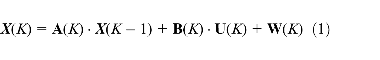
where the state vector
The errors that affect the accuracy and quality of the machined workpiece can be categorized as quasistatic errors and dynamic errors. 16 Quasistatic errors are those slowly varying errors between the workpiece and machine tool, such as geometric errors, cutting force–induced errors, fixturing errors, and thermal errors. Dynamic errors depend more on the operating conditions, such as spindle motion errors, vibrations, and controller errors. Quasistatic errors account for about 70% of the total errors of the machine tool. Therefore, the effects of locating errors, geometric errors of the machine tool, and tool deflection, which are the major error sources in a single machining process, are investigated in this article.
Modeling of the machining process
In this section, the definitions of coordinate systems and the assumptions used in this article are presented first. Then, the effects of the locating errors, geometric errors of the machine tool, and tool deflection on the machined surface are analyzed.
Coordinate systems and assumptions
To determine the positions of the cutting tool and workpiece in a machine tool, a series of coordinate systems should be defined first. As shown in Figure 1, the reference coordinate system (RCS) is fixed on the bed of the machine tool, and tool coordinate system (TCS) (OT-XTYTZT) is defined at the center of the tool. The ZT-axis of TCS is along the tool axial direction. In addition to those two coordinate systems, one coordinate system is fixed to each body in the kinematic chain. The details of the setup of these coordinate systems can be found in Figure 1(b).
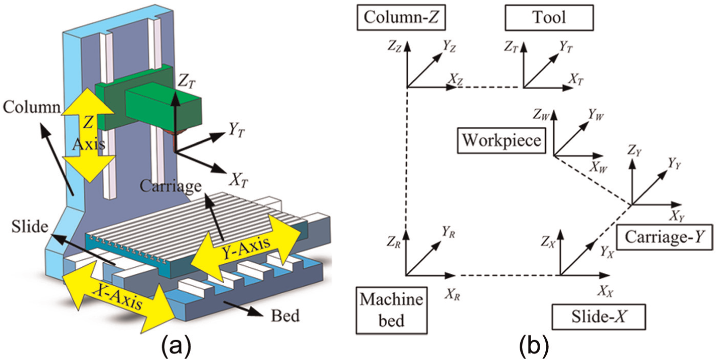
Coordinate frames of the machine tool: (a) configuration of the machine tool and (b) the setup of the coordinate systems.
To further simplify the modeling process, the following assumptions are introduced in the modeling process:
The workpiece, machine tool, and fixture are rigid; their deformations are ignored.
Defects on the workpiece and fixture are small.
The temperature is kept constant during the machining process; the thermal errors are ignored.
Backlash errors are ignored.
Use pins or plane surfaces as fixture locators.
Effects of locating errors
The fixture must satisfy the requirements of locating stability and total restraints to hold a workpiece. Due to the deviations on the fixture and the workpiece, the workpiece would deviate from its nominal position in the fixture. The translation and rotation deviations of the workpiece can be represented by a homogeneous transformation matrix
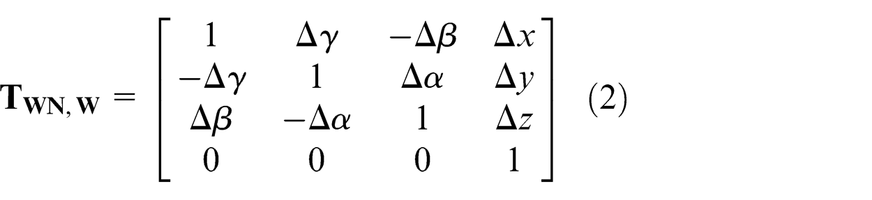
To obtain the parameters in
Determination of the difference face Λ. The difference face is defined as the difference between the fixture surface and datum surface: Λ = Λ d − Λ f .
Identification of the possible contact points. Construct the convex hull of Λ; the contact facet is the one which intersects the clamping force or the gravity. Its vertexes are the contact points.
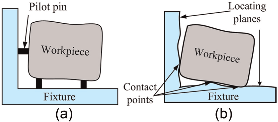
Locating errors of the workpiece: (a) fixture with pins and (b) fixture with locating planes.
For the ith contact point, the point on the datum is denoted as
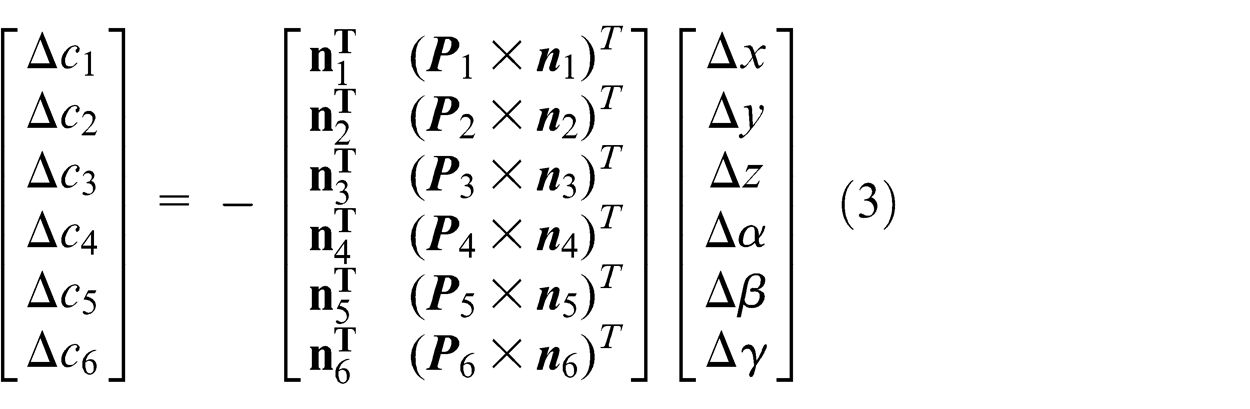
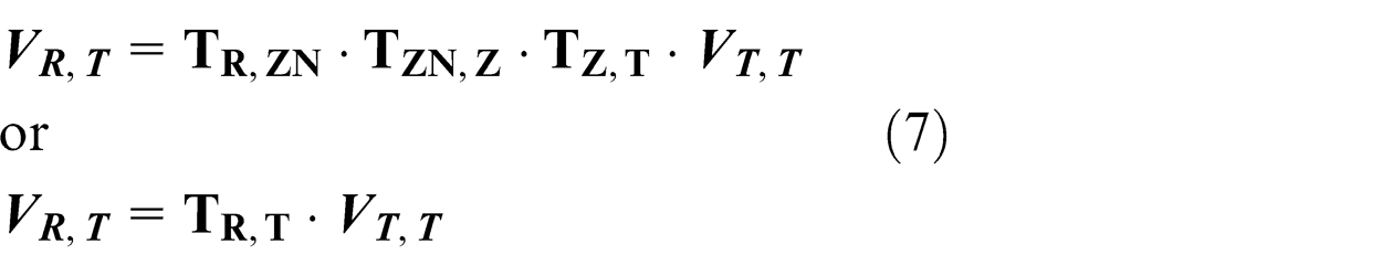
From equation (3), the parameters in equation (2) can be obtained. To evaluate the effects of geometric errors of machine tool and tool deflection on workpiece deviation, the coordinates of the workpiece should be further transformed from WCS to RCS
where
Effects of geometric error of machine tool
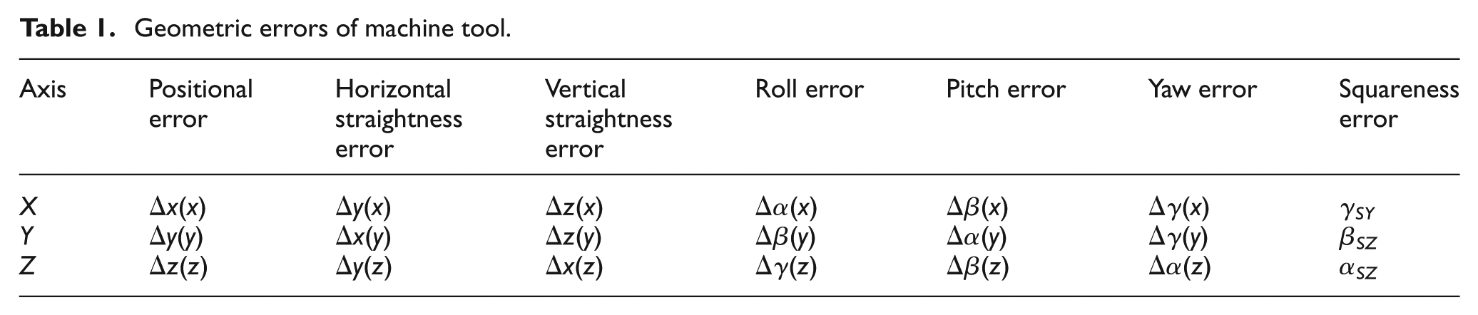
A three-axis machine tool has 21 independent geometric error components when the machine tool is considered as a set of rigid bodies. If a coordinate system is fixed to each of the three bodies in the machine tool, there are 6 errors per body or 18 errors. There also exist three squareness errors caused by non-orthogonality between the three axes. 18 All those geometric errors are listed in Table 1.
Geometric errors of machine tool.
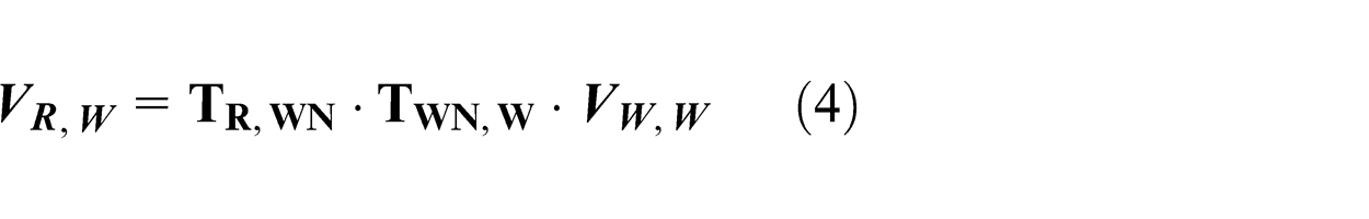
With consideration of these geometric error components, the coordinates can be transformed from WCS to RCS as
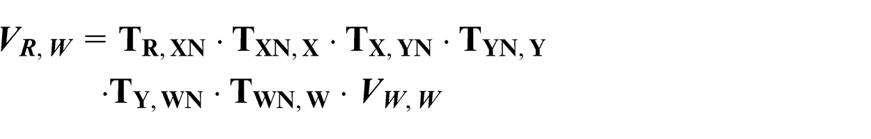
or
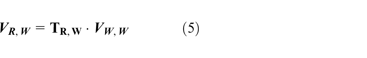
Details of the matrixes in equation (5) are presented as follows
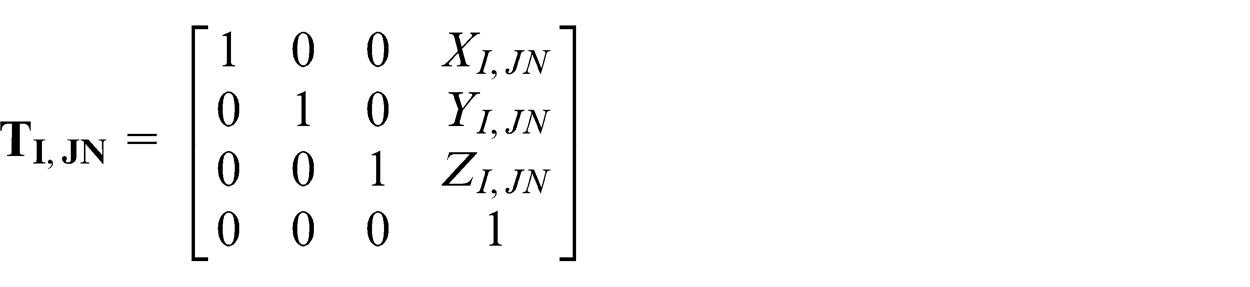
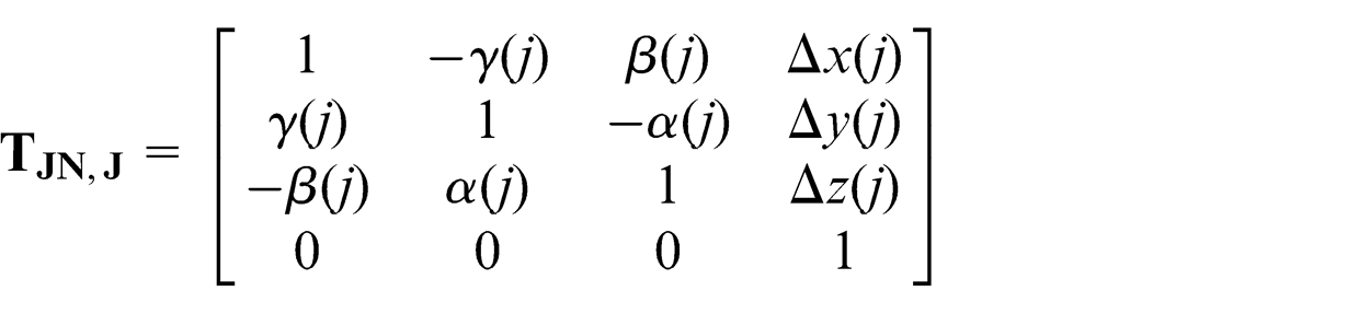
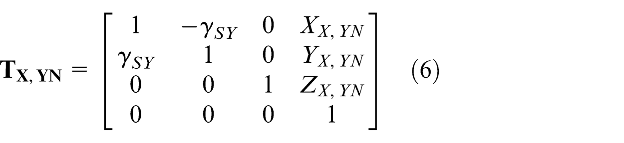
where (I,JN) = (R,XN), (Y,WN); (JN,J) = (XN,X), (YN,Y); (XI,JN, YI, JN , ZI,JN) represents the coordinate of the origin of JCS in ICS. And all the geometrical error components included in equation (6) can be obtained with the help of a laser interferometer or double ball bar.19,20 Similarly, the coordinates can be transformed from TCS to RCS as
As shown in Figure 3, when the tool is in cutting with the workpiece, the cutting edge would coincide with the points on the workpiece. Consequently, the points being cut can be expressed as
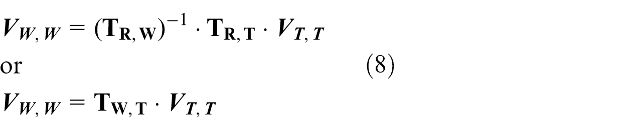
Contact points between the workpiece and the tool during a machining process.
Effects of tool deflection
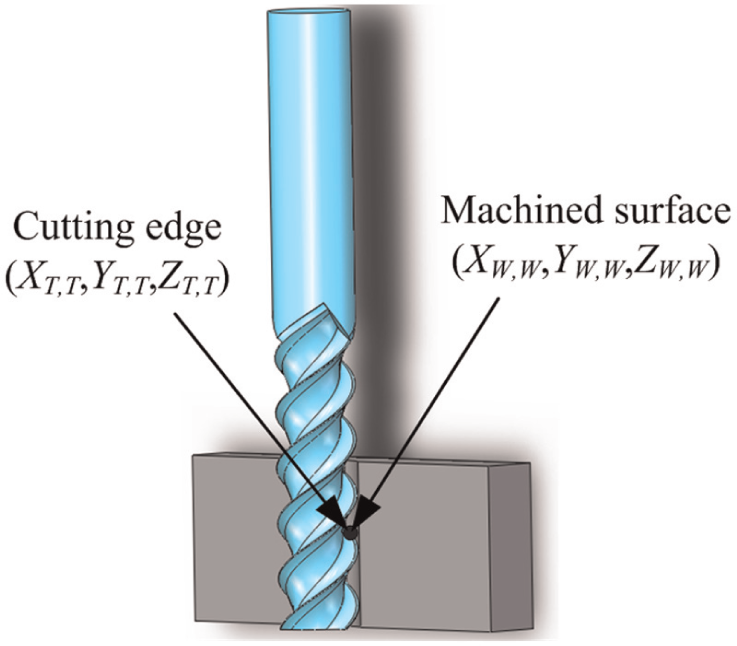
The cutting force has a significant influence on dimensional accuracy because of tool deflection in machining. 21 As shown in Figure 4, under the action of cutting forces, the tool will deviate from its nominal position. The deflection will be mapped on the machined surface. A peripheral milling tool is selected here to illustrate the effects of tool deflection on workpiece deviation.
Tool deflection in a machining process.
The geometry of a peripheral milling tool is shown in Figure 5. The radius, helix angle, and pitch angle of the tool are represented as r, β, and Φ p , respectively. To calculate the cutting force, the tool is divided into M equally spaced differential cutting elements along the axial direction. The thickness of each element is Δa = a/M, where a is the axial depth of cut. For the cutting element m, which is at elevation ZT,T = m·Δa, the immersion angle for the flute j is expressed as Φ j (m)
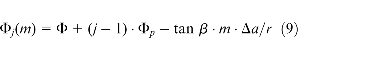
where Φ is the immersion angle for the first flute at the end of the tool. The instantaneous chip thickness for the cutting element m is
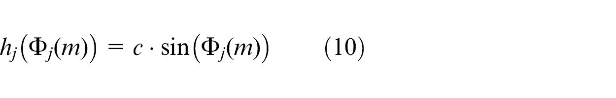
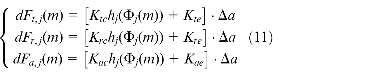
where c is the feed rate. The differential cutting forces for the flute j in the radial, tangential, and axial directions at cutting element m are calculated using the local cutting force coefficients (Krc, Ktc, Kac) and edge force coefficients (Kre, Kte, Kae) as 22
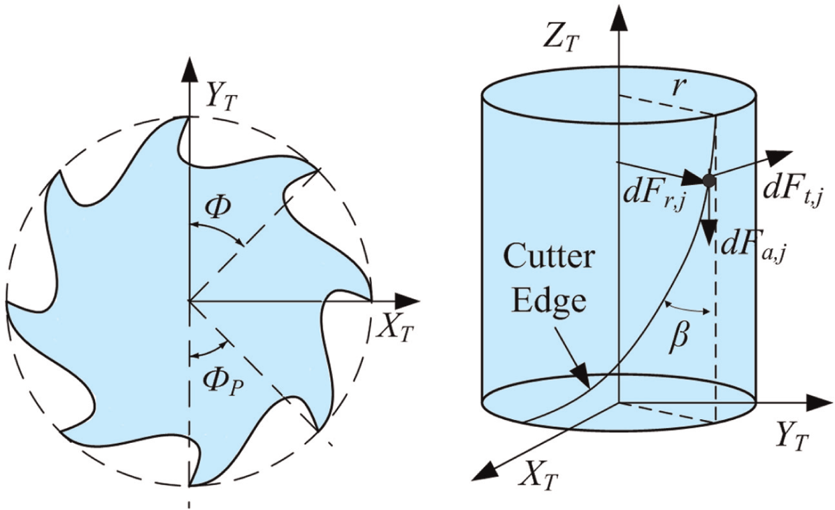
Geometry of a peripheral milling tool.
In equation (11), both the cutting force coefficients (Krc, Ktc, Kac) and edge force coefficients (Kre, Kte, Kae) can be obtained from orthogonal cutting tests using oblique cutting model. 22 The differential forces in radial, tangential, and axial directions can be transformed to TCS as
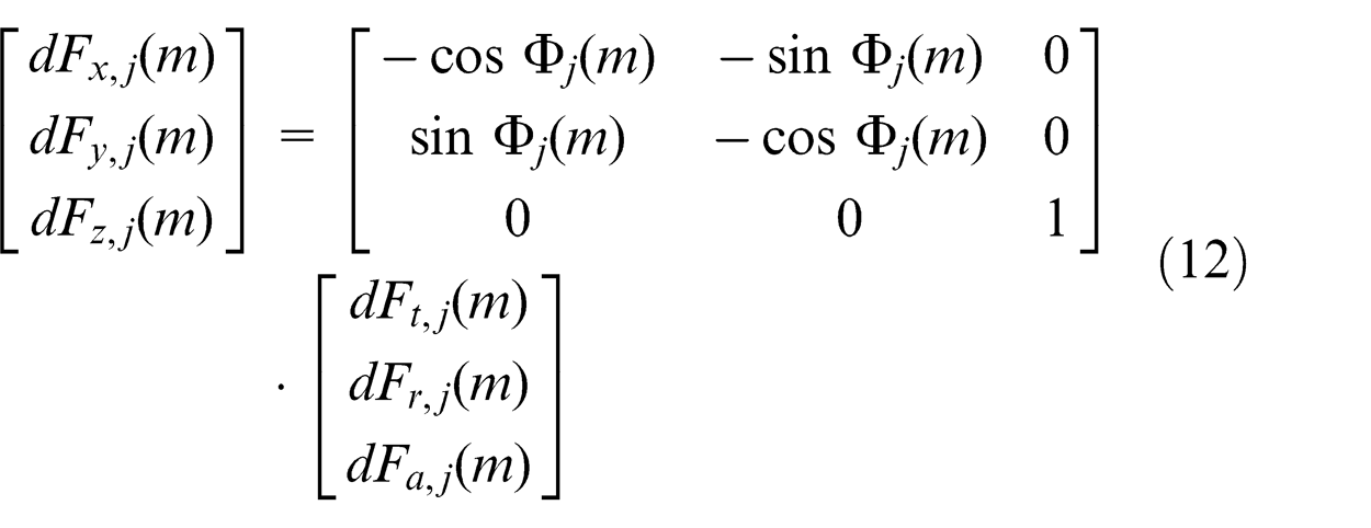
Substitute equations (10) and (11) into equation (12), and sum up the contributions of each cutting flutes. Then, the total differential forces for the cutting element m can be written as
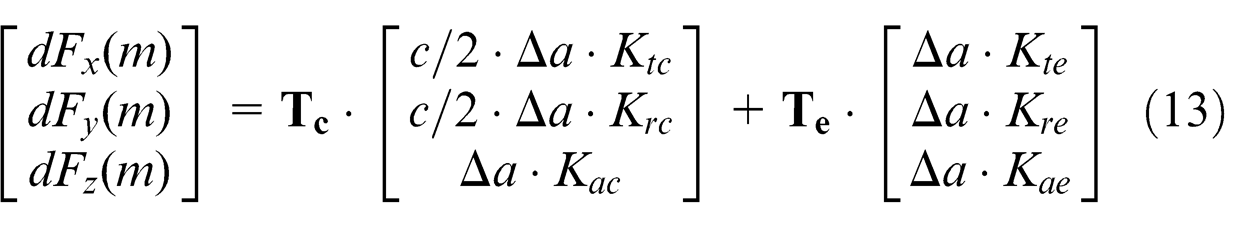
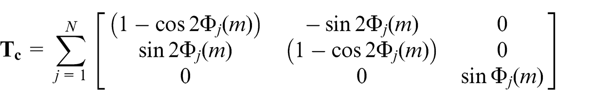
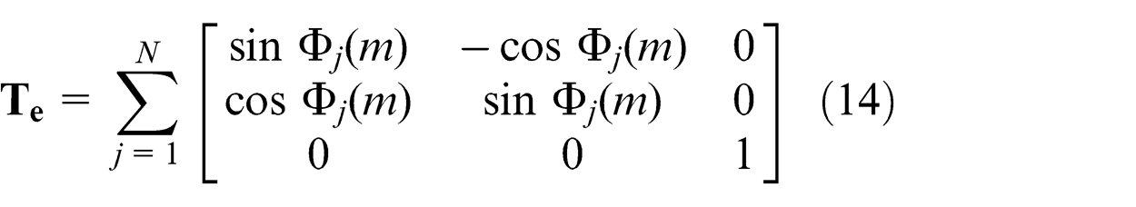
where
Integrate the differential forces acting on the cutting elements engaged with the workpiece, then the total cutting forces for the tool can be obtained.
The deflection of the tool at cutting element q caused by the forces applied at cutting element m is given using the cantilever beam formulation23,24
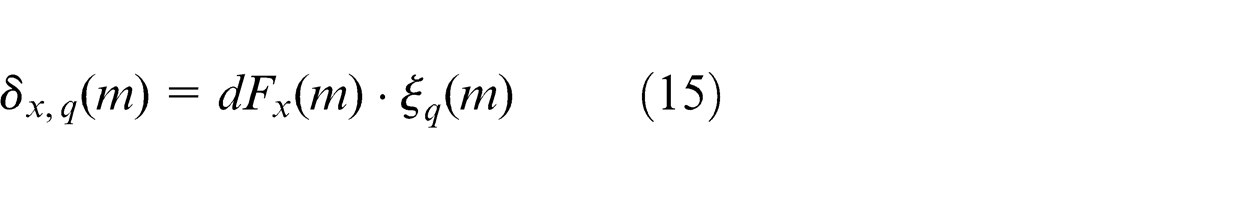
where
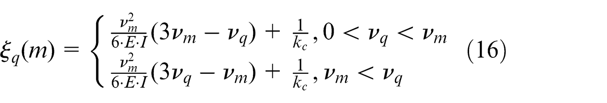
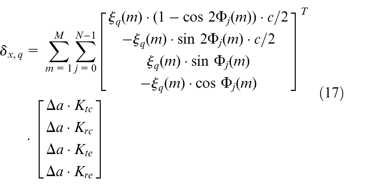
In equation (16), E is the Young’s modulus, I is the area moment of inertia of the tool, νm = L − m·Δa, L is the distance from the end of tool to the collet, and kc is the tool clamping stiffness in the collet. Consequently, the total deflection of the tool at cutting element q can be obtained by summing up the small deflections induced by each cutting elements engaged with the workpiece
Due to workpiece deviation, the engagement boundary will deviate from its nominal position. In Figure 6, the dot line represents the desired engagement boundary. When point A deviates from its nominal position to C, an additional cutting edge will be in cut with the workpiece. The thickness of this cutting edge can be approximated as ΔηA = ΔµA/tanβ, where ΔµA is workpiece deviation at point A. In Figure 7, b is the desired radial width of cut. The immersion angle for the cutting edge at the engagement boundary can be calculated as Φ E = asin((r − b)/r). Substitute this equation into equation (9), then the ZT coordinates of those additional cutting edges can be obtained.
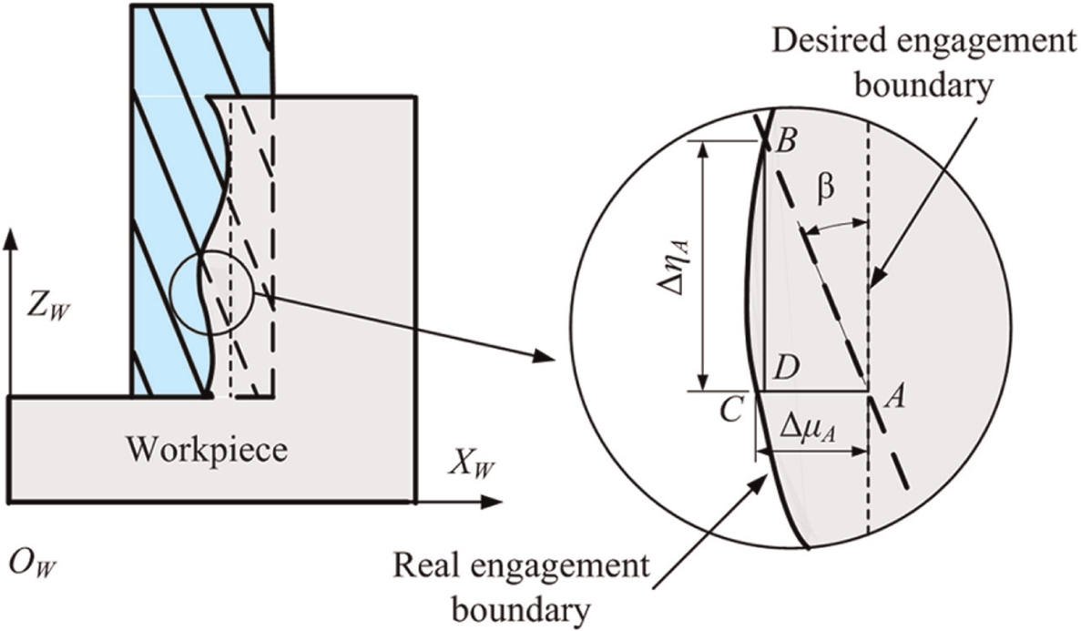
Engagement boundary.
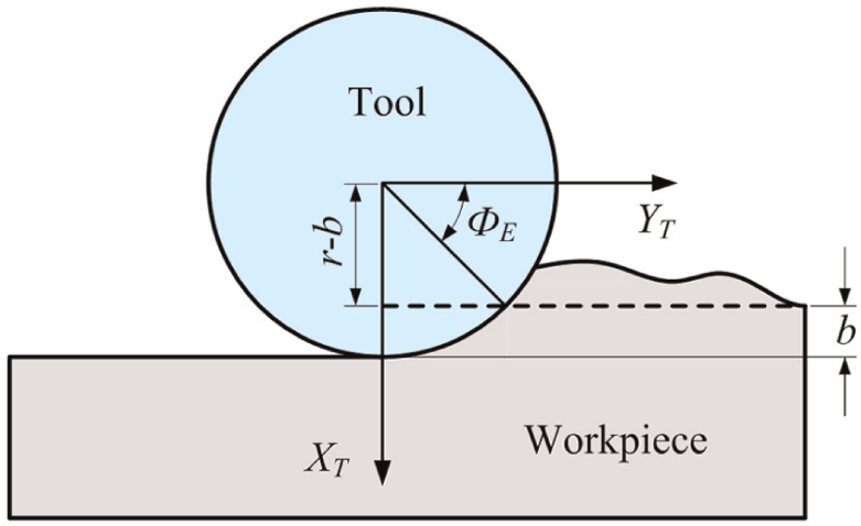
Immersion angle of the cutting edge at the engagement boundary.
Consequently, the additional deflection at cutting element q caused by the additional forces induced by workpiece deviation can be calculated as
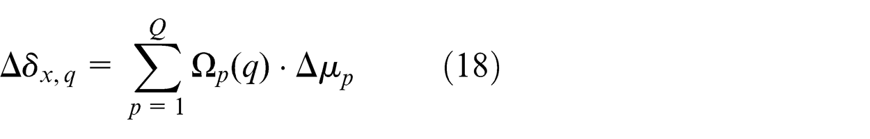
where
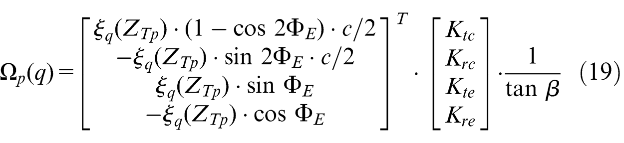
In equation (18), Q is the number of the additional cutting edges. ZTp represents their ZT coordinates. So, the total deflection of the tool at cutting element q can be expressed as
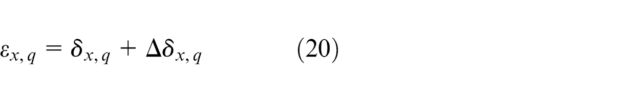
Taking the tool deflection into consideration, then equation (8) turns to be
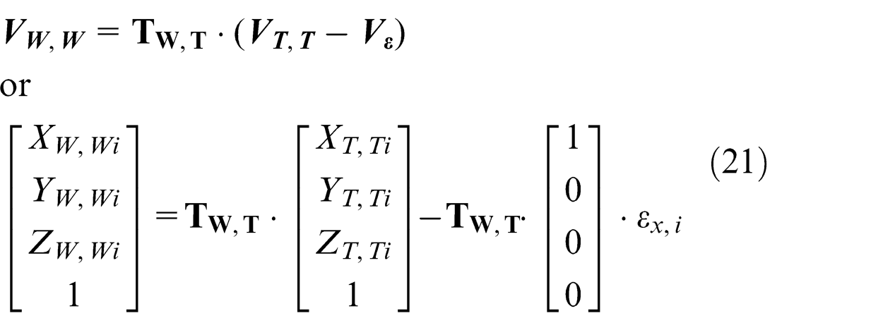
Substitute equations (18) and (20) into equation (21)
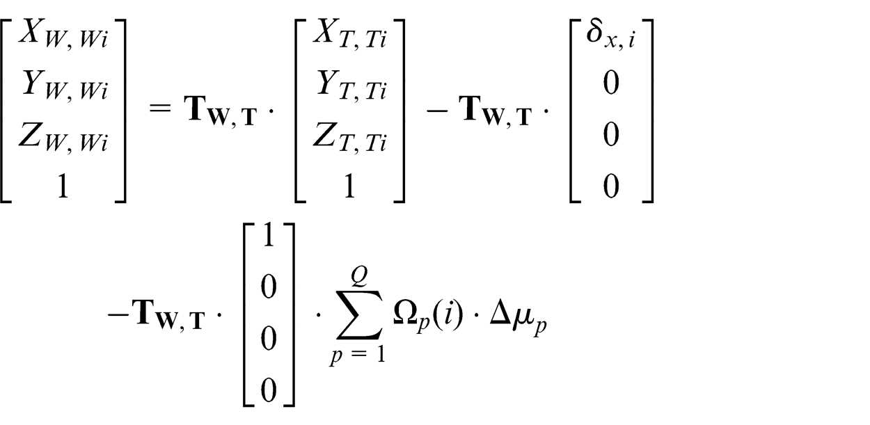
Δµp can be expressed as the difference between the real and nominal coordinates of the workpiece
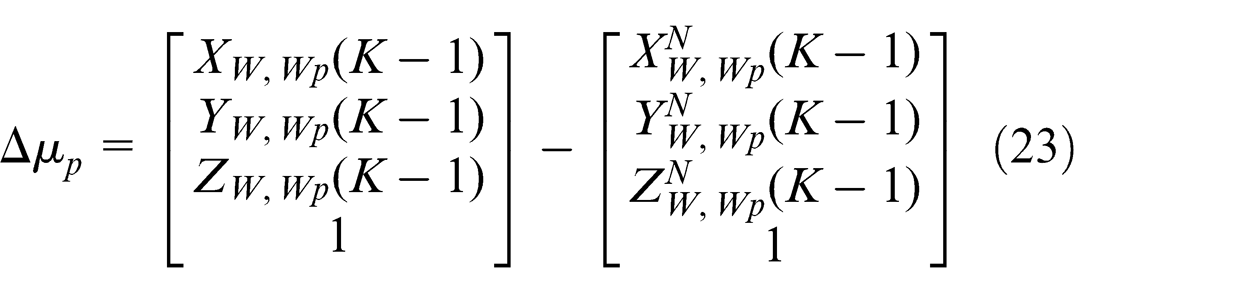
Then
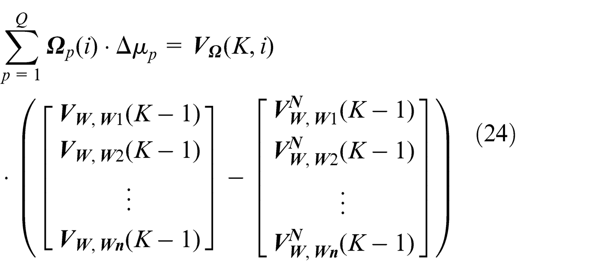
where
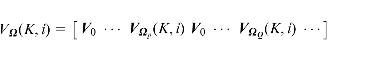
The place of
where
Modeling of variation propagation between different passes
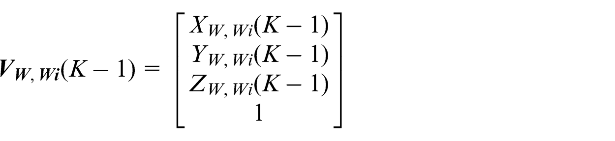
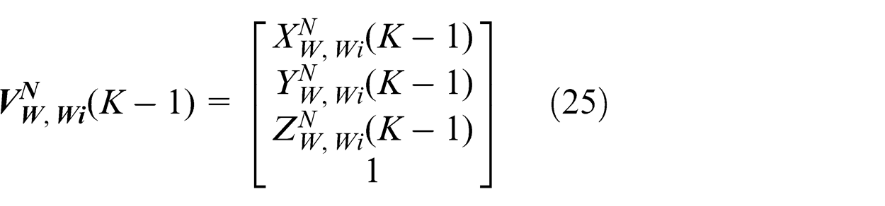
Workpiece deviation is defined as the difference between the real and nominal coordinates of the machined workpiece. It can be expressed as
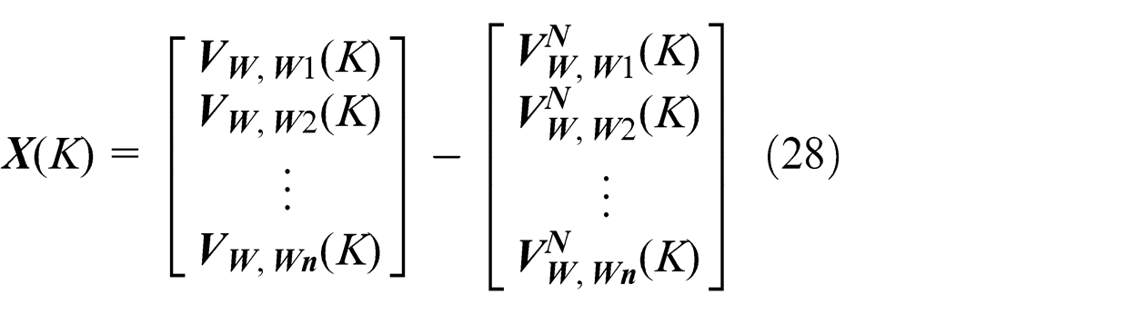
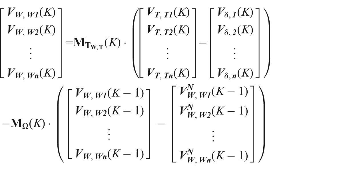
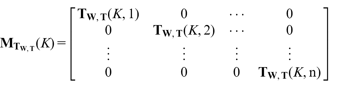
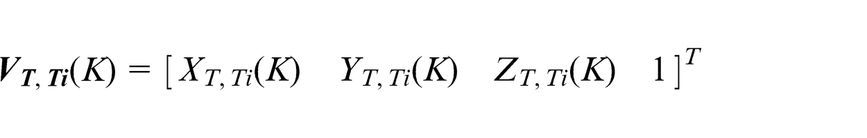
Substitute equation (28) into equation (26)
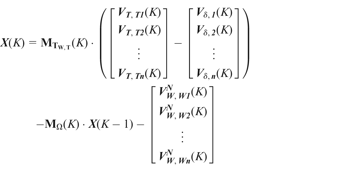
Compare equation (29) with equation (1)
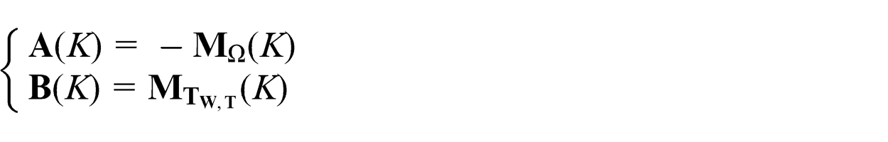
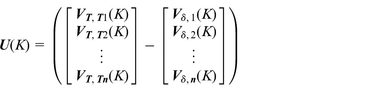
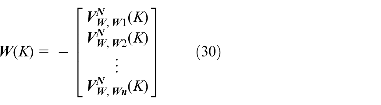
From equation (29), it can be found that workpiece deviation after the Kth pass is mainly determined by three components, that is,
Case studies
To validate the proposed model and its application in cutting parameters optimization, several simulations have been conducted in MATLAB R2007b. In this section, some results are presented and analyzed.
The frames of the rough workpiece and the fixture used in the simulations are shown in Figure 8. Plane MW is the surface to be machined. Plane DW is the measurement reference. CW is the primary locating datum. AW is the secondary locating datum. The deviation of the rough workpiece and the fixture are simulated as:
CW ∼ N(0, 0.033 mm)
AW and BW ∼ N(0, 0.033 mm)
MW ∼ N(0, 0.033 mm)
AF and DF ∼ N(0, 0.005 mm)
BF and CF ∼ N(0, 0.005 mm)
where N(µ,σ) represents the normal distribution, µ is the mean value, and σ is the standard deviation.
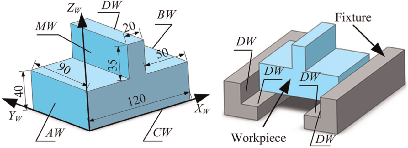
3D view of the workpiece and fixture.
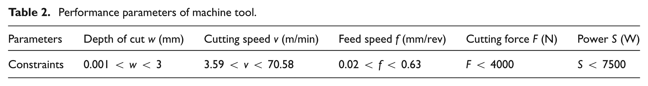
A XA-5032 type milling machine is selected to execute the operations. The performance parameters of the machine tool are listed in Table 2.
Performance parameters of machine tool.
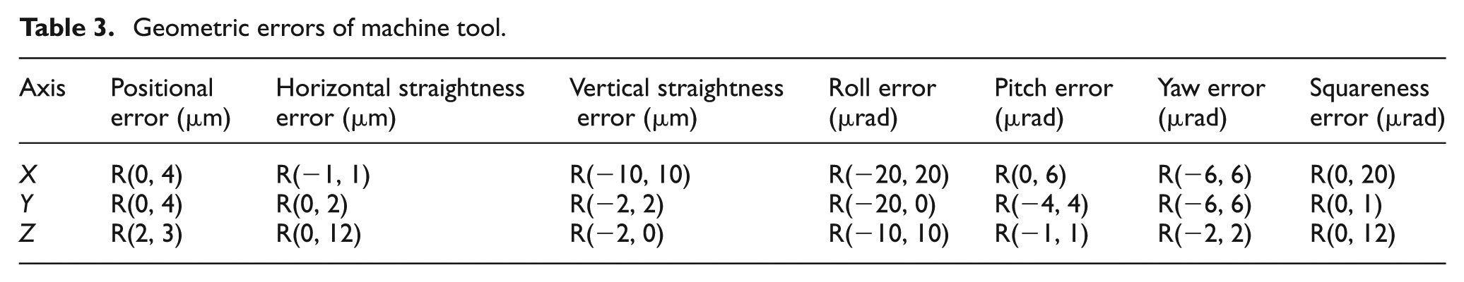
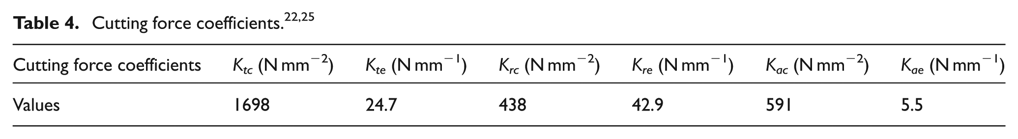
The geometric errors of the machine tool are listed in Table 3. The material of the workpiece is Ti6AL4V, Young’s modulus of the tool is 620 GPa, the diameter of the tool is 19.05 mm, helix angle is 30°, and the tool gauge length is 55.6 mm; the cutting force coefficients are shown in Table 4.
Geometric errors of machine tool.
Model validations
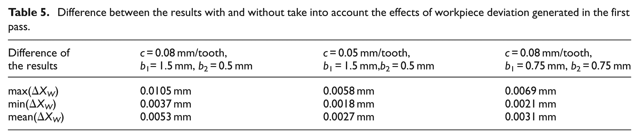
Three groups of simulations are conducted to illustrate the effects of workpiece deviation generated in the previous pass on workpiece deviation produced in the next pass. For each group, the rough workpiece is machined by two passes of milling. The total radial width of cut is 2 mm. Details of the cutting parameters used in the simulations are listed in Table 5.
Difference between the results with and without take into account the effects of workpiece deviation generated in the first pass.
In each group, two simulations are conducted:
Simulation which takes into account the effects of workpiece deviation generated in the first pass.
Simulation without taking into account the effects of workpiece deviation generated in the first pass.
The differences of the results are shown in Figure 9. The maximum, minimum, and mean values of those differences are also listed in Table 5.
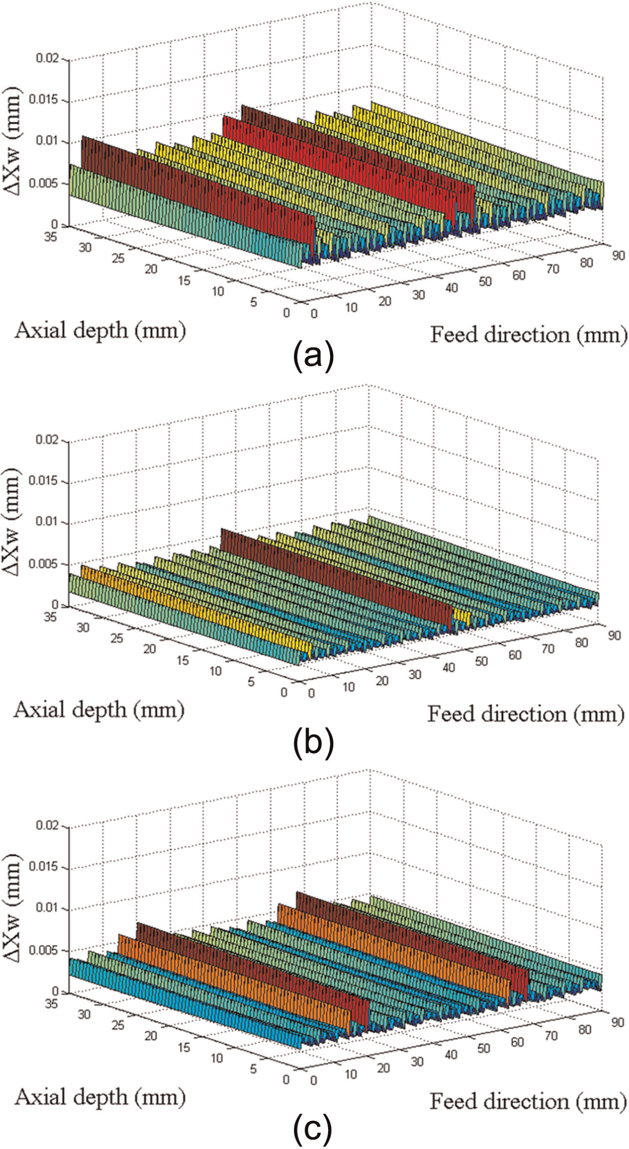
Differences between the simulation results with and without taking into account the effects of workpiece deviation generated in the first pass: (a) c = 0.08 mm/tooth, b1 = 1.5 mm, b2 = 0.5 mm; (b) c = 0.05 mm/tooth, b1 = 1.5 mm, b2 = 0.5 mm; and (c) c = 0.08 mm/tooth, b1 = 0.75 mm, b2 = 0.75 mm.
From the results listed in Table 5, the difference values are mainly determined by the cutting parameters. The effects of the cutting parameters on workpiece deviation are further analyzed in section “Effect of the cutting parameters.”
Effect of locating errors and geometric errors of the machine tool
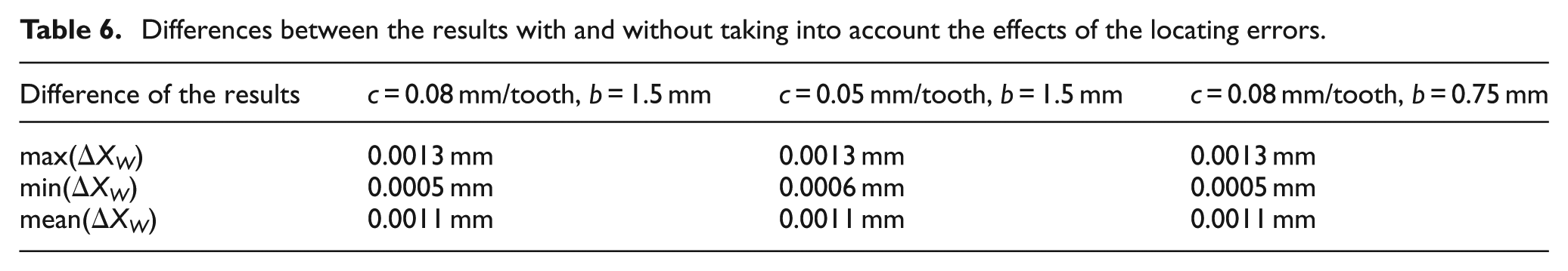
Three groups of simulations are conducted to illustrate the effects of locating errors and geometric errors of the machine tool. In Figure 10, all the results are obtained at c = 0.08 mm/tooth and b = 0.75 mm (the third cases of Tables 6 and 7). Figure 10(a) shows workpiece deviation when both the effects of locating errors and geometric errors of the machine tool are considered. Figure 10(b) shows the differences of workpiece deviation with and without taking into account the effects of the locating errors. Figure 10(c) shows the differences of workpiece deviation with and without taking into account the effects of the geometric errors of the machine tool. The maximum, minimum, and mean values of those differences are listed in Tables 6 and 7.
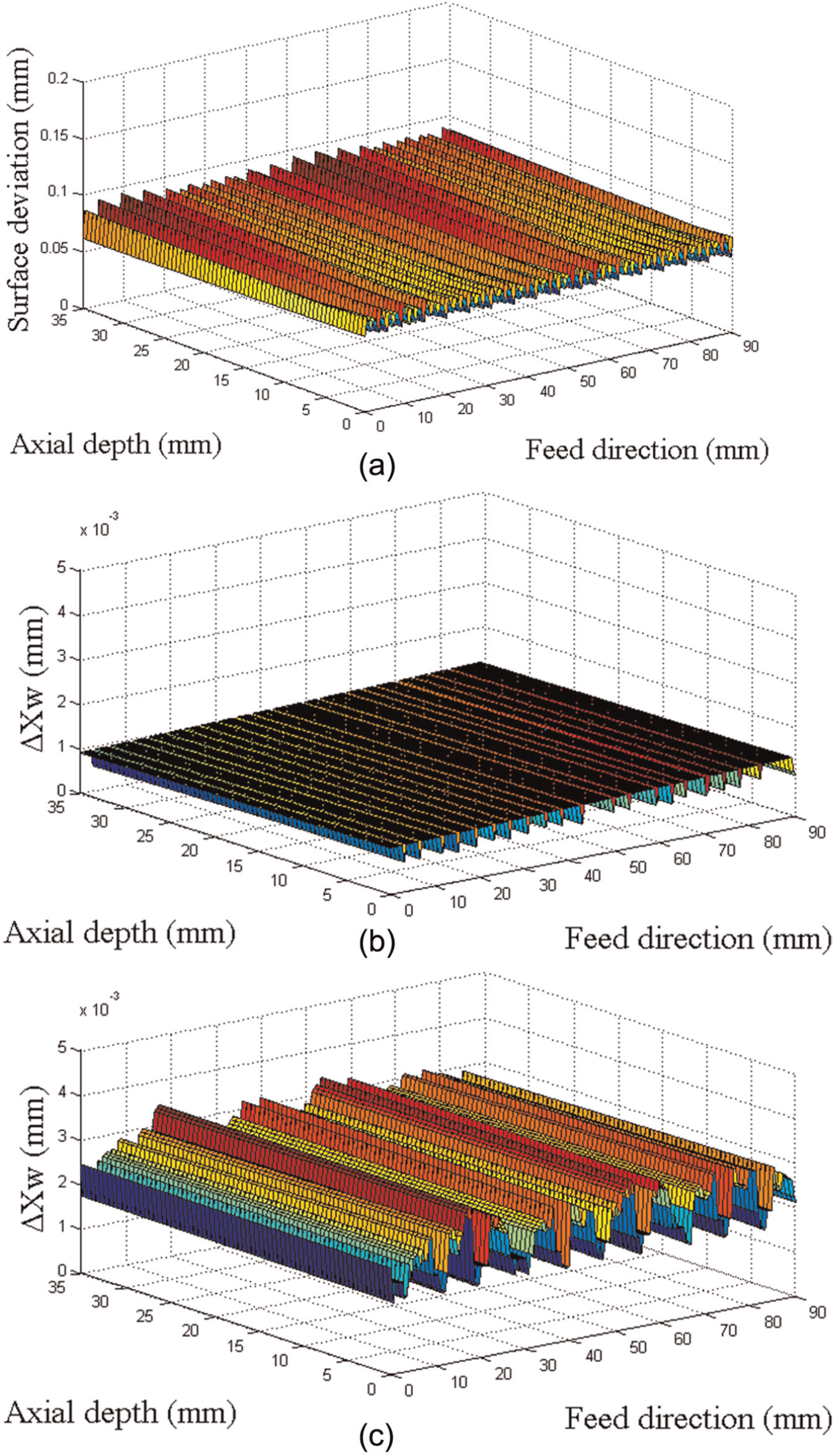
Simulation results at c = 0.08 mm/tooth, b = 0.75 mm: (a) workpiece deviation with taking into account both the effects of locating errors and geometric errors of machine tool, (b) the difference between the simulation results with and without taking into account the effects of the locating errors, and (c) the difference between the simulation results with and without taking into account the effects of the geometric errors of the machine tool.
Differences between the results with and without taking into account the effects of the locating errors.
Differences between the results with and without taking into account the effects of geometric errors of the machine tool.
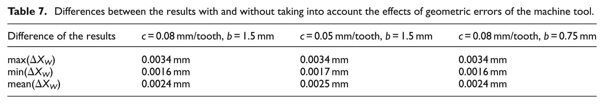
In a multi-stage machining process, the workpiece will be located and relocated on different fixtures. Therefore, the locating errors and geometric errors of the machine tools will be changed from one stage to another. But for a single machining process, when the fixtures and machine tool are selected, the locating errors and geometric errors of the machine tool are kept unchanged. And that is why the difference values for different cutting parameters listed in Tables 6 and 7 are rarely changed. Compared with the total deviation of the workpiece (in Figure 10(a)), those difference values listed in Tables 6 and 7 are rarely small. That is mainly because the locating errors and the geometric errors of the machine tool (Table 3) are set very small.
Effect of the cutting parameters
Another two groups of simulations are conducted to illustrate the effects of the cutting parameters on workpiece deviations: (1) simulations with fixed radial width of cut (cutting board) and (2) simulations with fixed feed rate per tooth. The calculated results are presented in Figure 11.
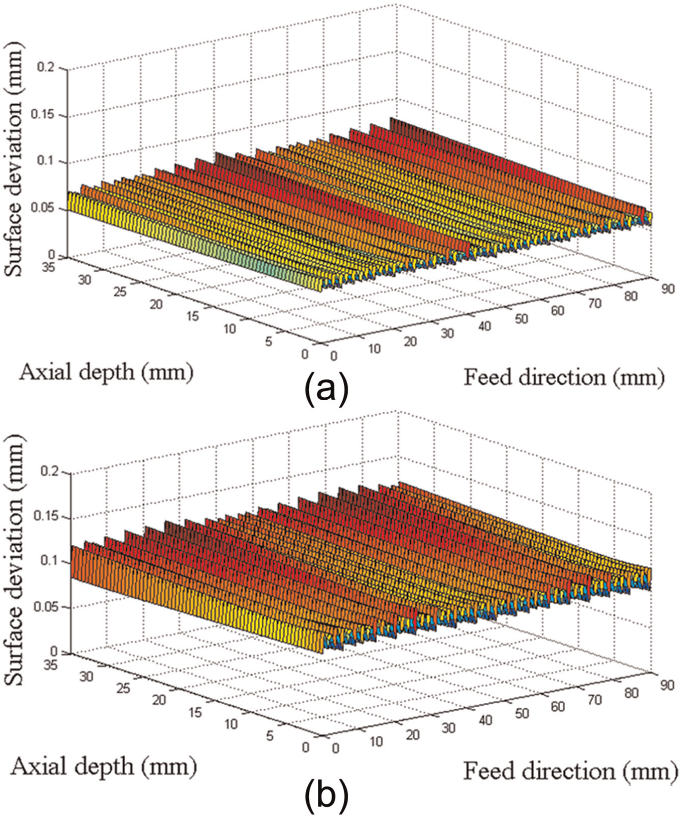
Workpiece deviations at different cutting parameters: (a) c = 0.08 mm/tooth, b = 0.5 mm and (b) c = 0.1 mm/tooth, b = 1 mm.
As shown in Figure 12(a), when the radial width of cut is fixed, workpiece deviation and feed rate show a linear relationship. This is because equation (17) is a linear function of feed rate c.
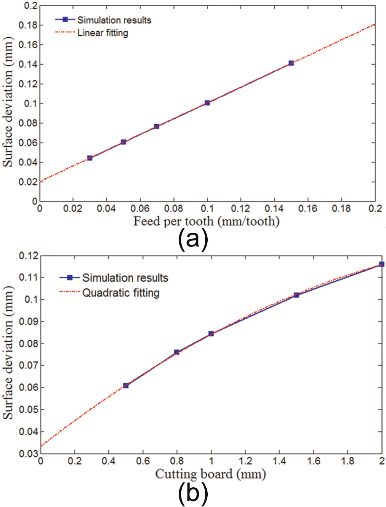
Mean values of workpiece deviation: (a) b = 1 mm and (b) c = 0.08 mm/tooth.
When feed rate is fixed, workpiece deviation and the radial width of cut can be approximated by a quadratic equation (Figure 12(b)). This quadratic relationship can be explained by the term cos(2Φ E ) in equation (19). It can be transformed to a quadratic function of the radial width of cut.
From the above results, workpiece deviations at different cutting parameters can vary in a region 0.04–0.14 mm. This region is large enough to make a main influence on the form and dimensional deviations of the workpiece.
Applications
In production, manufacturers always seek for optimal cutting parameters to reduce cutting time and improve the accuracy of the workpiece. Usually, the cutting time or cutting cost is selected as the objective function. The acceptance rate of the product is assumed to be high enough to meet the requirements of the process tolerance. Because there are various errors in a machining process, this assumption cannot always be satisfied. Using the model proposed in section “Modeling of variation propagation between different passes,” the manufacturers can make an estimation of the acceptance rate of the machined workpiece and the distribution of workpiece deviation. Therefore, as an application, the proposed model will be applied in the cutting parameters optimization in this section.
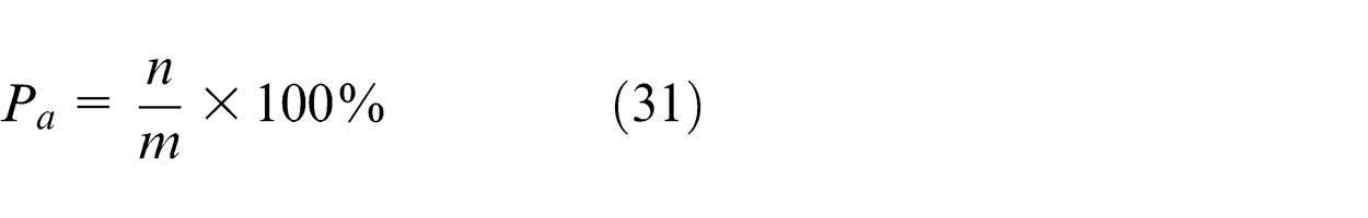
The workpiece shown in Figure 8 is supposed to be machined by three passes, and the total radial width of cut is 3 mm. The dimensional errors are desired to be limited in the range of −0.04 to 0.04 mm, and the form tolerance is 0.05 mm. The acceptance rate Pa of the machined workpiece can be calculated as
The total cutting time t is
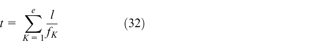
where subscript K represents the Kth pass, l is the pass length, fK (mm/min) is the feed speed in the feed direction for the Kth pass, m is the size of the rough workpiece used in the simulation, and n is the number of the machined workpiece which meets the requirements of the tolerance.
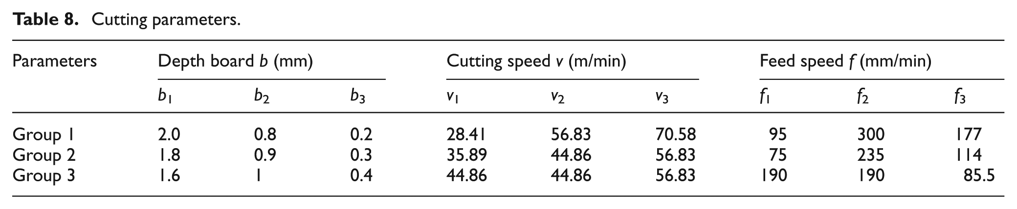
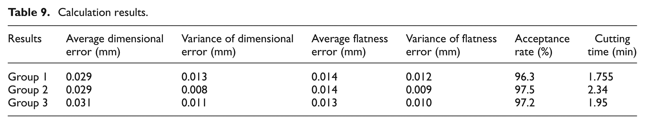
In this article, m is set to 1000. Three alternative groups of cutting parameters are listed in Table 8. The simulation results are shown in Table 9. In those three groups, Group 1 gives less cutting time. Group 2 provides a higher acceptance rate. The results of Group 3 are between them. According to those results, the manufacturer can properly select a group of cutting parameters based on the requirements of the production. With overall consideration of both the cutting time and acceptance rate, the cutting parameters listed in Group 3 are more reasonable selections in this case. Since more information are provided before the machining process, the potential loss can be avoided or reduced to an acceptable level, and the requirements of the manufacturers can be satisfied.
Cutting parameters.
Calculation results.
Conclusion
A variation propagation model for a single machining process with multi-passes was proposed in this article. This model integrates the effects of the locating errors, geometric errors of machine tool, and tool deflection on workpiece deviation. Different with the multi-stage process, the locating errors and geometric errors of the machine tool will not be changed in a single machining process. The effects of locating errors and geometric errors of the machine tool on workpiece deviations of different passes are kept unchanged. For a single machining process with multi-passes, workpiece deviation generated in the previous pass will affect the next pass. Therefore, the radial width of cut for the next pass is changed. Consequently, the cutting forces for the next pass are changed. Under the action of cutting forces, the tool would deviate from its nominal position. The tool deflection is mapped on the machined workpiece. The deviation of newly machined surface will further affect the following pass. This process will be continued until all the passes are finished. Since the effects of workpiece deviation generated in the previous pass on the next pass are included, the relationships between different passes are established using the derived model. To validate this model, groups of simulations are conducted. From the results of those simulations, the effects of workpiece deviation generated in the previous pass on workpiece deviation produced in the next pass are observed; and the effects of locating errors, geometric errors of the machine tool, and the cutting parameters on workpiece deviation are validated. As an application, the proposed model was used in the cutting parameters optimization at the end of this article. The proposed model provides a building block for multi-stage machining process. If the locating and relocating errors between different stages are included, the proposed model can be further developed to describe the variation propagation phenomenon in multi-stage machining processes.
Footnotes
Appendix 1
Declaration of conflicting interests
The authors declare that there is no conflict of interest.
Funding
This research was supported by the Science Fund for Creative Research Groups of National Science Foundation of China (No. 51221004), and the National Nature Science Foundation of China (No. 51275464) and the National Basic Research Program of P. R. China (973 Program, No. 2011CB706505).