
Abstract
Ti–6Al–4V, as one of the most frequently used titanium alloy in aerospace applications, is characterized by its excellent mechanical and corrosion properties. However, it is well known that Ti–6Al–4V is difficult to be formed at room temperature. Therefore, hot stretch bending has been used to improve formability and reduce springback in forming Ti–6Al–4V profile. In the virtual development of designing suitable hot stretch bending processes for Ti–6Al–4V, numerical simulations are considered desirable. However, the reliability of numerical simulations depends on the models and methods used as well as the accuracy of material data. In this work, a set of uniaxial tension tests was performed on Ti–6Al–4V at the temperatures ranging from 923 to 1023 K and strain rate from 0.005 to 0.05 s−1. Moreover, a set of stress relaxation tests was conducted on Ti–6Al–4V at the temperature range between 773 and 973 K and pre-stretch elongation ranging from 0.7% to 10%. The Johnson–Cook and Arrhenius models were used to characterize the uniaxial tension and the stress relaxation behavior, respectively. Finite element model of hot stretch bending was created according to the laboratorial experiment setup in ABAQUS based on the constitutive models calculated above. The finite element simulation indicates that the residual stress in the profile decreases greatly in the secondary stage of hot stretch bending due to the stress relaxation behavior. The predicted springback shows promising agreement with the corresponding experimental observations.
Keywords
Introduction
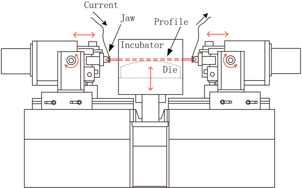
Titanium and titanium alloys are excellent candidates for aerospace applications due to their high strength-to-weight ratio, excellent corrosion resistance and composite compatibility. 1 However, titanium alloy is difficult to form into complex configurations, especially at room temperature. Forming processes at elevated temperature are required to produce titanium components. 2 Superplastic forming (SPF) is used to form complex-shaped titanium components based on the phenomenon of superplasticity at high temperatures. The temperature for SPF of Ti–6Al–4V ranges from 1143 to 1193 K.3,4 Hot forming is often used to form titanium sheets in aerospace under the temperature range from 773 to 973 K. 5 In recent years, several new processes have been developed to form titanium alloy sheet at elevated temperature. Highly achievable strains and flexible manufacturing methods make the hot incremental sheet forming (HISF) an alternative process to hot forming of titanium alloy sheets.6–9 Hot stretch bending (HSB) was proposed for bending forming of elongated metal parts. In the HSB process, creep forming is induced after the workpiece was wrapped against the die by maintaining the position of jaw for a selected dwell time. At the same time, the temperature is controlled as needed.10,11 The forming cycle of HSB is shown in Figure 1.
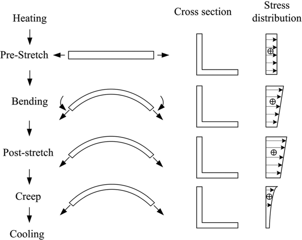
Forming cycle of hot stretch bending (HSB).
During the HSB cycle, the workpiece is heated to the temperature between 753 and 973 K or above. Once the working temperature has been reached, the workpiece is stretched and wrapped against the die while the working temperature is controlled as required. After position feedback indicates that the workpiece has arrived at its final position, the control system maintains the position of jaw for a selected dwell time to induce creep forming. Then, the workpiece is allowed to cool at a controlled rate. Once the temperature has arrived at its final set point, the force on the workpiece is released and the heating source stops. The workpiece is allowed to free cooling to room temperature. 12
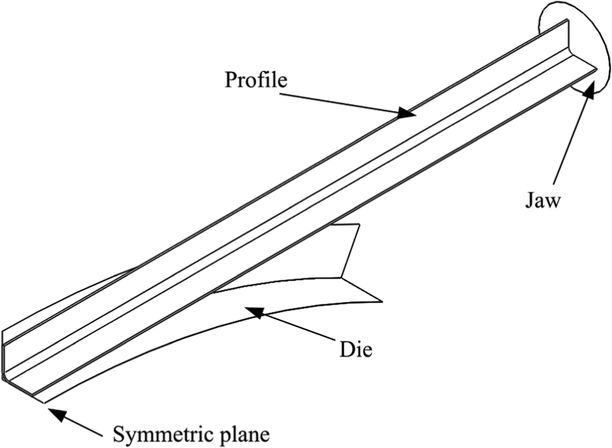
The fundamental of HSB is illustrated in Figure 2, where
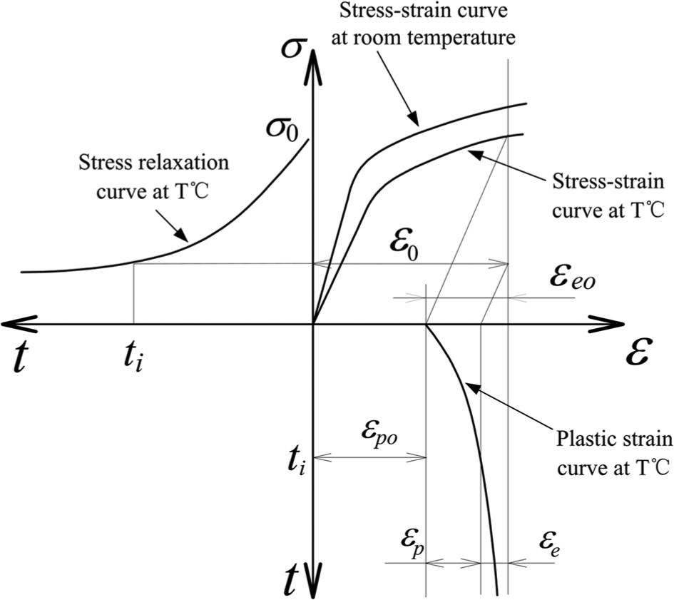
Fundamental of hot stretch bending (HSB).
It can be seen from Figure 2 that the fundamental of HSB is pursuing lower residual stress and smaller springback by stress relaxation process during the creep period. The HSB process allows the benefits of stretch forming and creep forming, including inexpensive tooling and good repeatability.
Finite element (FE) simulations are extensively used in metal-forming industry, where this technology has contributed to a better understanding of forming processes and reduce the time-consuming and costly die tryouts.13,14 However, the reliability of the numerical simulations depends not only on the models and methods used but also on the accuracy and applicability of the input data. Creating as little deviance as possible between the FE model and the experimental setup is a prerequisite for the correlation between predicted and measured values. Many research efforts have been focused on this issue. Li et al. 15 discussed the computational details of a viscoplastic FE analysis of three-dimensional SPF in conical bulging and rectangle box bulging. The verification test of conical bulging indicates that the accuracy of the FE modeling of SPF depends on the constitutive model and optimum pressure cycle. Accurate material parameters play an especially crucial role in numerical modeling. Wang et al. 16 established a two-dimensional nonlinear thermo-mechanical coupled FE model for the vacuum hot bulge forming of BT20 alloy cylindrical workpiece to calculate the temperature and deformation fields. The results show that with the increase in temperature, the plastic strain increases and the residual stress decreases under the same technological condition. Odenberger et al.17,18 carried out a set of material tests at elevated temperatures to generate experimental reference data for FE-analyses of sheet metal forming of Ti–6Al–4V. The predicted responses show promising agreement with the corresponding experimental observations when the anisotropic properties of the material are considered. The yield surface shape has been found important and the accuracy of the predicted shape deviation could be slightly improved by including the cooling procedure.
As there are two stages in the HSB process, FE model should simulate these two stages together. This work is dedicated to the modeling of stretch bending and creep forming in the HSB process. A set of uniaxial tension tests was performed on Ti–6Al–4V at the temperatures ranging from 923 to 1023 K and strain rate from 0.005 to 0.05 s−1. Moreover, stress relaxation tests were performed on Ti–6Al–4V at the temperatures ranging from 773 to 973 K and pre-stretch elongation ranging from 0.7% to 10%. Johnson–Cook (JC) and Arrhenius equations were used to characterize hot tension and stress relaxation behavior, respectively. FE model of HSB was created in ABAQUS based on the constitutive models calculated above, and the predicted springback is compared with the corresponding experimental observations.
Material and experiment
Materials
The Ti–6Al–4V alloy sheet was hot-pressed into profile parts with the cross section shown in Figure 3 for the HSB validation tests. The length of the profile is 950 mm.
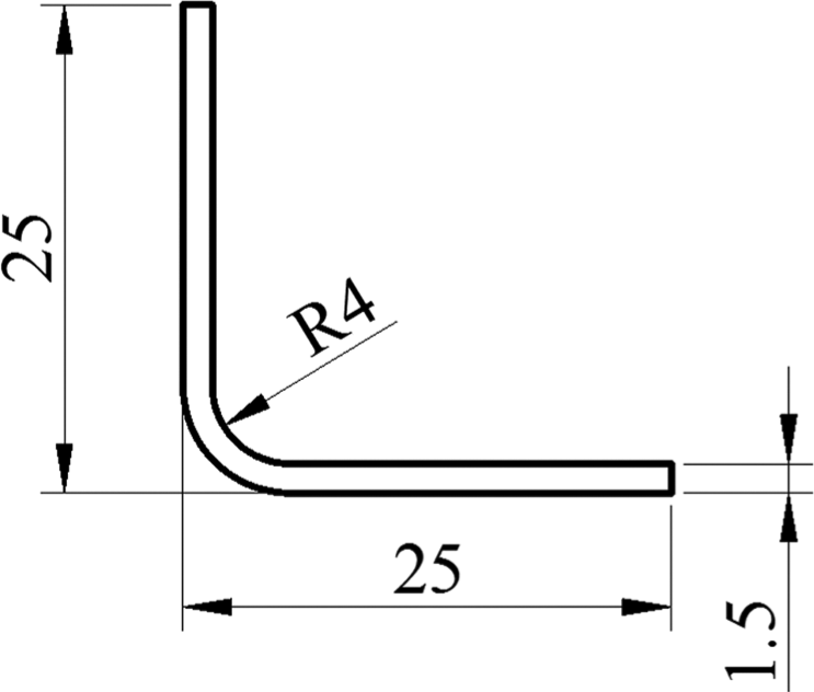
Cross section of profile parts.
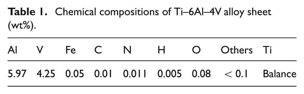
The chemical composition of the Ti–6Al–4V alloy sheet is listed in Table 1.
Chemical compositions of Ti–6Al–4V alloy sheet (wt%).
The initial hot treatment condition of the Ti–6Al–4V alloy sheet was annealed after rolling. The microstructure of the alloy is shown in Figure 4.
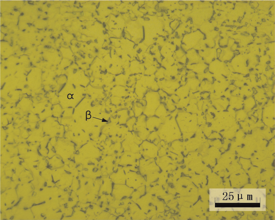
Initial microstructure of the Ti–6Al–4V alloy.
The material used in uniaxial tensile tests and stress relaxation tests is the same batch of Ti–6Al–4V alloy sheet as that used in HSB validation tests. The specimen was prepared by laser cutting process in the rolling direction, keeping the tensile direction consistent with the longitudinal direction.
Experimental procedures
Uniaxial tensile tests
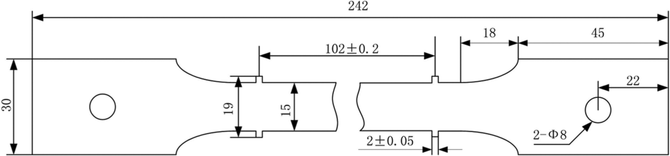
The uniaxial tensile tests were performed on the Zwick/Roell Z100 electric universal testing machine equipped with a furnace composed of three independent heating zones. The furnace has a constant temperature zone 30 cm long and offers possibility to control the atmosphere temperature with ±3-K precision. Prior to the uniaxial tensile tests, the specimens were heated to the deformation temperature at a rate of 20 K/min. The geometry of the uniaxial tensile test specimen is shown in Figure 5.
Geometry of uniaxial tensile test specimen.
The tests were performed at temperatures of 923, 973 and 1023 K and the strain rates of 0.005, 0.01 and 0.05 s−1 according to “ISO 6892-2.” 19 Finally, the engineering curves obtained from the uniaxial tensile tests were converted into true stress–strain curves.
Stress relaxation tests
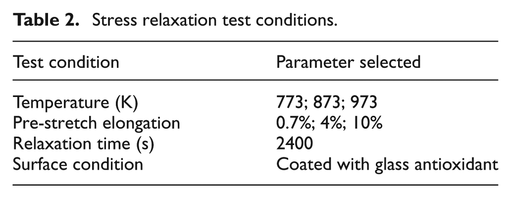
The stress relaxation tests were carried out on RWS-50 Electronic Creep Testing Machine following “ASTM E328.” 20 The test condition is listed in Table 2, and the test procedure is described as follows:
Position the specimen.
Furnace heating to desired test temperature at a rate of 2 K/s. Meantime, the drawing force (≤10 MPa) was applied on the specimen.
Maintain test temperature for 2 h.
Pre-stretch the specimen to desired elongation in a short time (≤5 s).
Maintain the needed elongation for 2400 s and record the force during the relaxation time.
Stress relaxation test conditions.
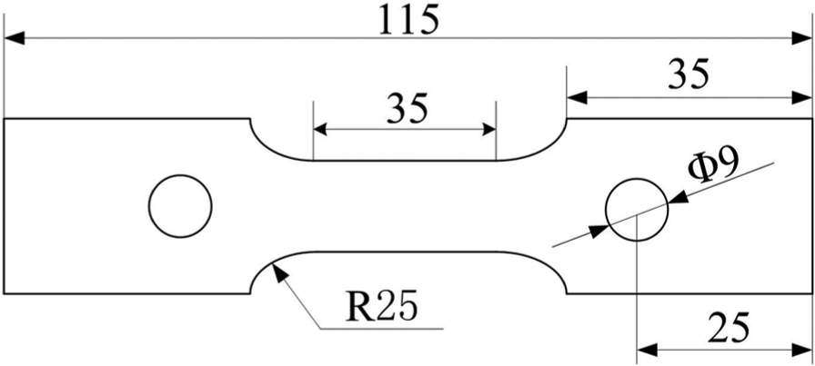
The geometry of the stress relaxation test specimen is shown in Figure 6.
Geometry of the stress relaxation test specimen.
Validation tests of HSB process
Laboratory tests were constructed to validate the accuracy of FE prediction of HSB process, as shown in Figure 7.
HSB of titanium alloy profile at elevated temperature.
In order to prevent heat dissipation, the profile part was covered by Asbestos blanket. The die was pre-heated to the desired temperature before the HSB process by flame heating. Then, the profile was loaded and heated to the desired temperature by the resistance heating equipment. The thermocouple was coated with insulating layer and installed on the middle of the part. The heating equipment works with the proportional–integral–derivative (PID) closed-loop control system, which can adjust the current in the part to maintain the stability of the part temperature. The deformation sequence of HSB process is described as follows:
The part was pre-stretched to 0.67% to reach the yield point of the Ti–6Al–4V alloy.
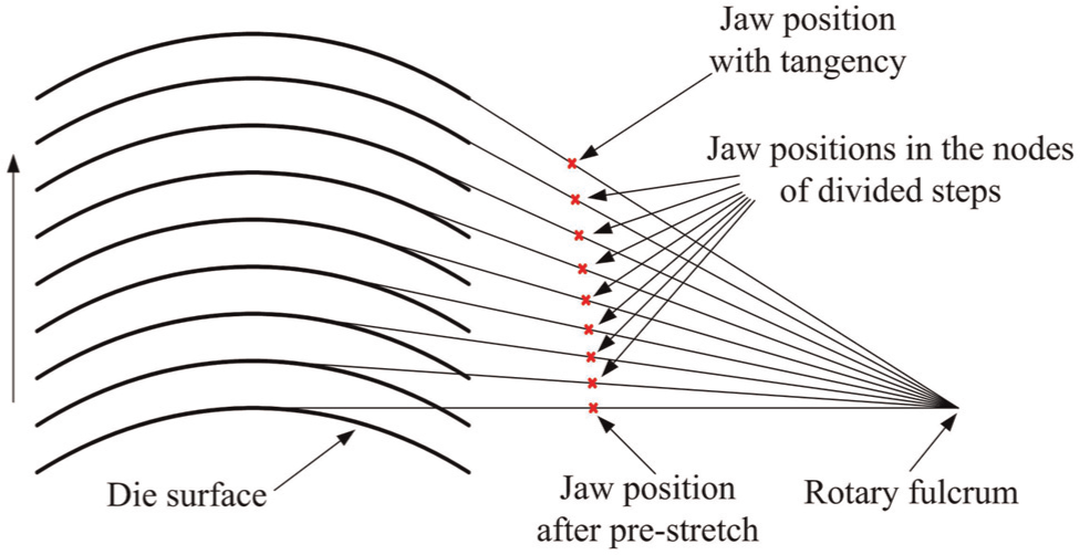
The die rises with a speed of 25 mm/min. Meantime, the jaw moves and rotates to cooperate with the deformation of the part to maintain the elongation of the neutral layer in the part. According to the dimension of the profile part, die and equipment, the profile part will be wrapped against the die perfectly when the die shifts upward 397.2 mm. In order to set the jaw position in the control system, the displacement of the jaw is divided into eight steps. Each step is 50 mm except the last step, 47.2 mm. The jaw positions in the nodes of the divided steps were input to the control system. The detailed position of the jaw will be calculated automatically in the control system by linear interpolation. The analytic geometry figure of the movement is expressed in Figure 8.
The spacing distance of the die in the rise direction is set as 50 mm except the last step, 47.2 mm.
The part was post-stretched for 0.6% elongation after the bending process.
Maintain the part against the die for a selected dwell time, while the temperature is controlled at the desired temperature to induce stress relaxation in the profile part.
The part was allowed to cool at a rate of 2 K/s. Once the temperature has arrived at 473 K, the jaw opened and the force on the part was removed. Then, the part was allowed to free cool to room temperature.
Analytic geometry figure of the jaw in HSB.
In this work, the temperature is 973 K and the dwell time is 0 s (no stress relaxation process), 600 s and 1200 s. Because the profile part used in the validation test is expensive, the amount of the parts is limited. The tests were performed twice under the condition of 973 K and 1200 s relaxation time. The results seem close to each other. So, the validation tests in other conditions were performed once in this work.
To measure the springback of the profile parts after the HSB, an articulated arm with the model RA-7525 SI was used to scan the surface of the die and profile parts. There are some section distortions in the part after springback, which is shown in Figure 9. The distortion is uniform in the length direction. The reason may be attributed to the particular stress distribution in the part. However, the measured area for the springback evaluation in this article is limited to a small area, which is shown in Figure 10. So, the section distortion behavior does not affect the springback measurement. This article researches the springback behavior of the part after the HSB process. So, the distortion is not considered here.
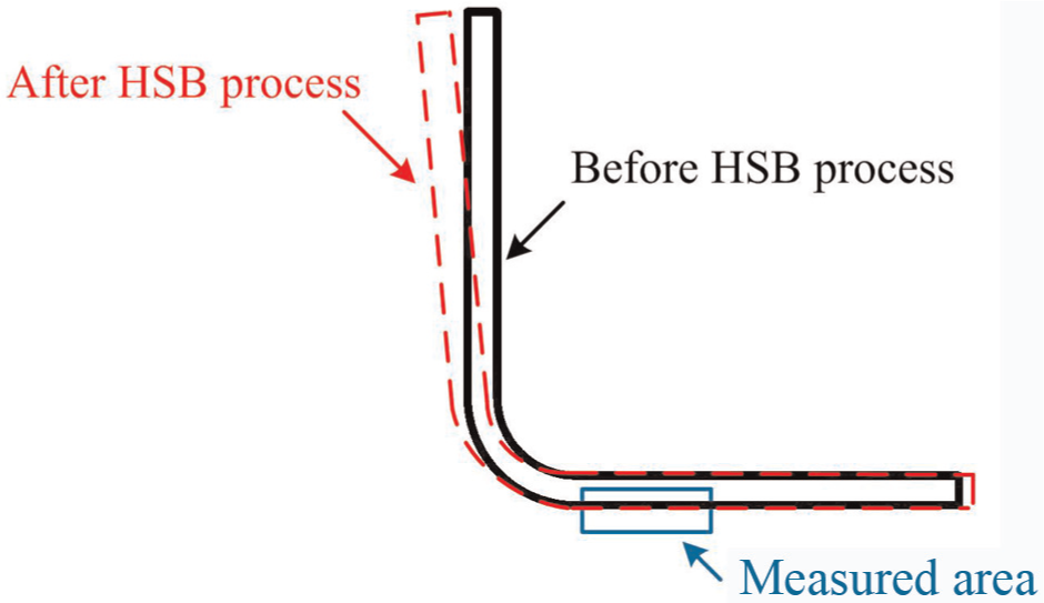
Section distortion in the profile part.
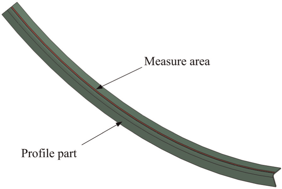
Measured area on the profile part.
The die surface was fitted reversely in Geomagic Studio after the point cloud data were obtained. The error of fitting process is 0.009 mm, which indicates it is highly reliable. Then, the point cloud of the profile part was compared with the die surface to calculate the gap between them in Spatial Analyzer.
Constitutive modeling
Constitutive modeling for the stretch bending process
The results of uniaxial tensile tests at the temperature of 923–1023 K and strain rate 0.005–0.05 s−1 were shown in Figure 11.
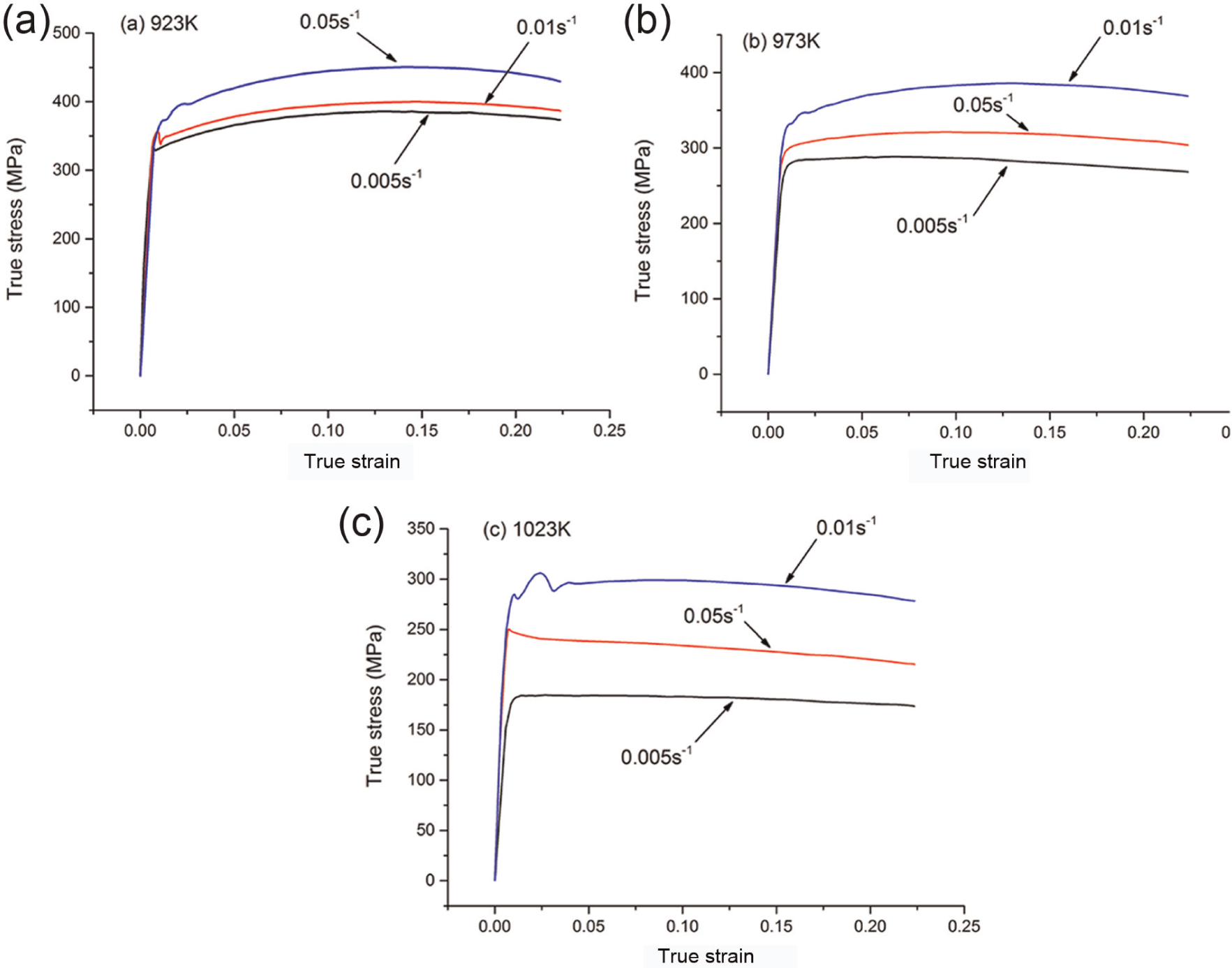
True stress–strain curves for different strain rates: (a) 923 K, (b) 973 K and (c) 1023 K.
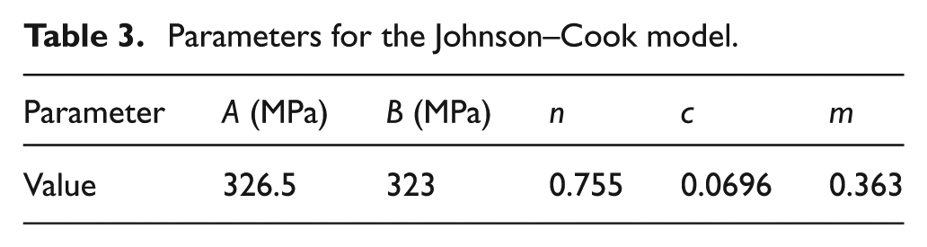
Among the empirical and semi-empirical models, the JC model was used for a variety of materials with different ranges of deformation temperature and strain rates.21–24 The JC model can be expressed as 25
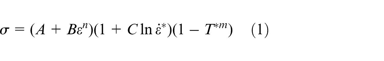
where
In this work, 923 K is taken as the reference temperature and 5 × 10⁻³ the reference strain rate. Equation (1) can be reduced to
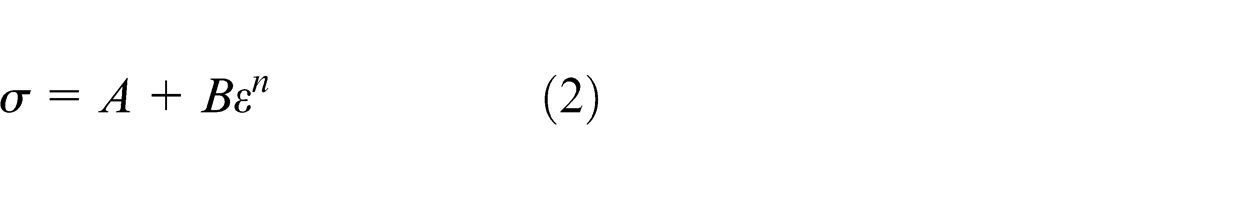
Taking natural logarithm of equation (2), equation (3) can be obtained as follows
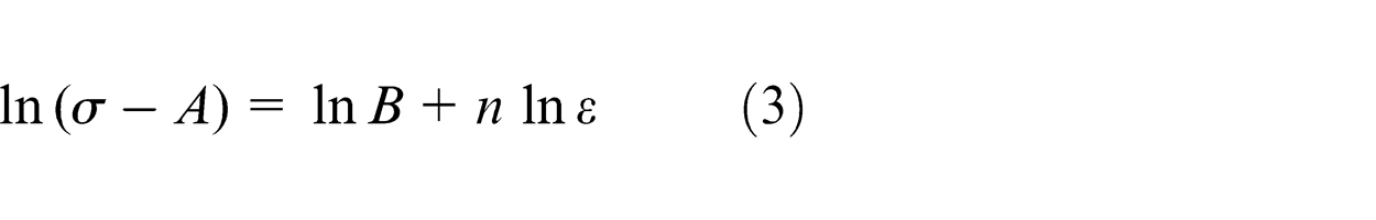
The value of
Relationship between
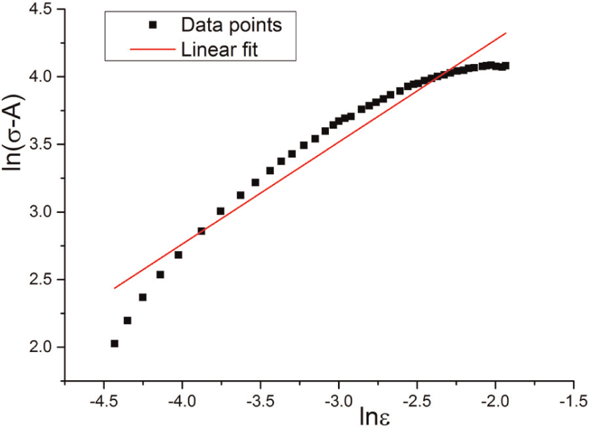
When the deformation temperature is 923 K, equation (1) can be written as
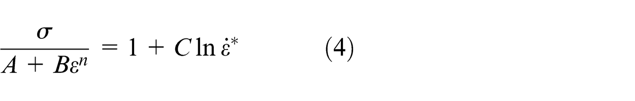
It can be seen form equation (4) that the value of C can be obtained from the average slope of straight lines which present the relationship between
Relationship between
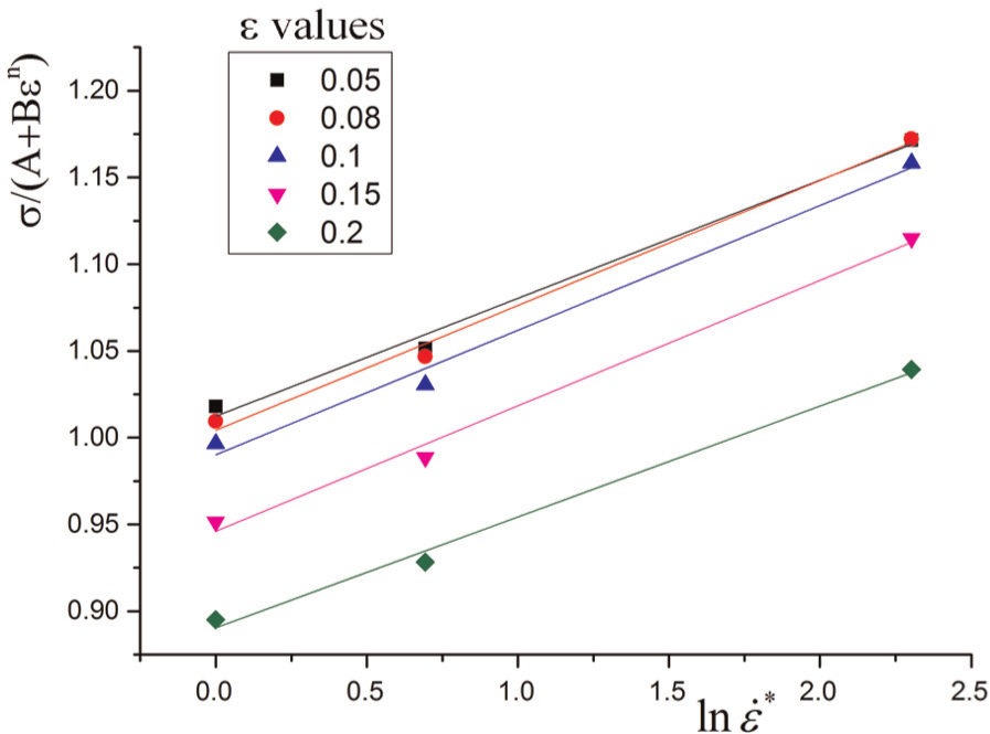
Similarly, at reference strain rate, equation (1) can be expressed as
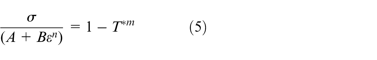
Taking natural logarithm of equation (5), equation (6) can be obtained as
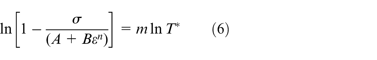
The material constant
Parameters for the Johnson–Cook model.
Constitutive modeling for the stress relaxation process
The true stress–time curves during the relaxation period are presented in Figure 14.
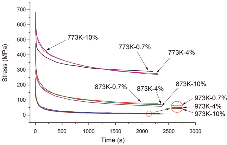
True stress–time curves for different temperatures and pre-stretch elongation.
Figure 14 shows that the stress curves are close to each other for the same temperature, especially for 973 K. The pre-stretch elongation has little effect on the relaxation process under the same temperature.
The relationship between the creep strain rate and stress, which is the basic relationship for the stress relaxation process, can be obtained from the stress relaxation experiment. For the stress relaxation process, the following equation is obtained
where
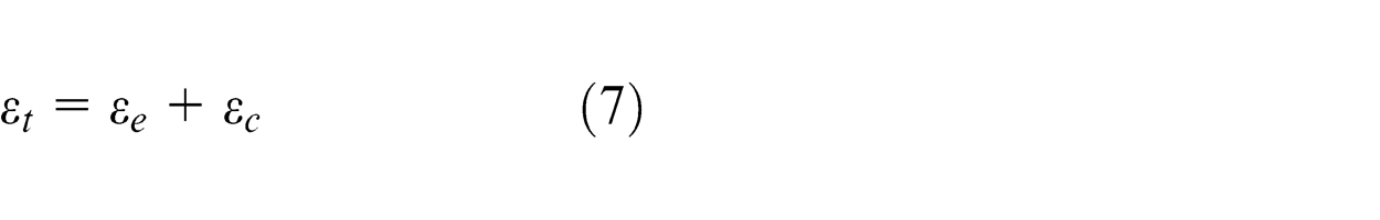
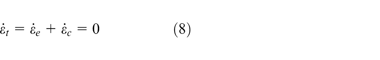
In the stress relaxation process, the total strain remains constant, and the elastic strain transforms to the creep strain. Then, equation (8) can be obtained as
The creep strain rate can be expressed as
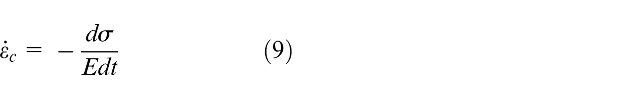
where
In order to obtain the relationship between the creep strain rate and stress, exponential decay function with the form in equation (10) was employed to fit the stress curve in Figure 14
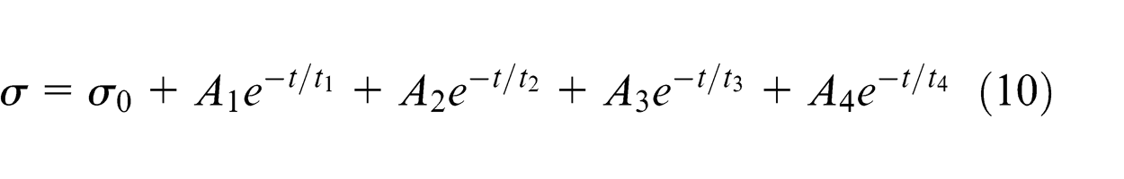
where
Parameters of the exponential decay function
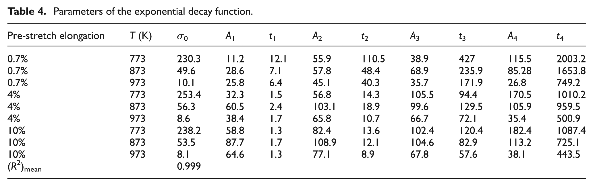
In this work, a mean R 2 of 0.999, which states the fitting precision, indicates that the exponential decay function agrees very well with the experimental data. The comparisons between the fitted and experimental data are shown in Figure 15.
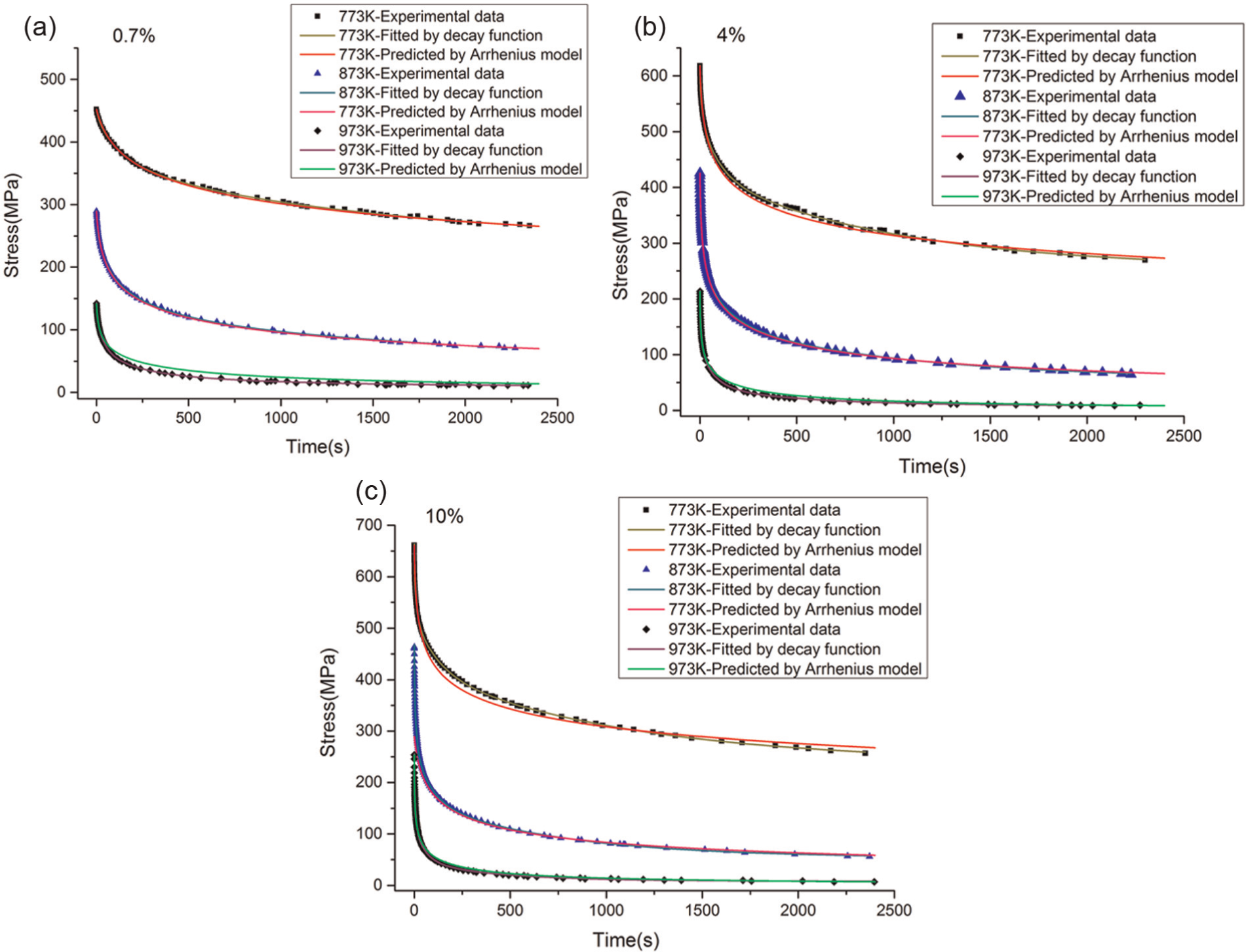
Comparison among fitted, predicted and experimental data: (a) 0.7%, (b) 4% and (c) 10%.
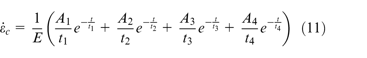
After deriving calculus to equation (10), the creep strain rate can be obtained from equation (11)
Therefore, the relationship between the creep strain rate and stress can be obtained. The Arrhenius equation was selected to describe this relationship in the finite element method (FEM) code. The effects of the temperature and strain rate on the deformation behaviors can be characterized by Zener–Hollomon parameter in an exponential equation. The hyperbolic law in Arrhenius-type equation gives better approximations between Zener–Hollomon parameter and flow stress.26–28 The two equations are mathematically expressed as
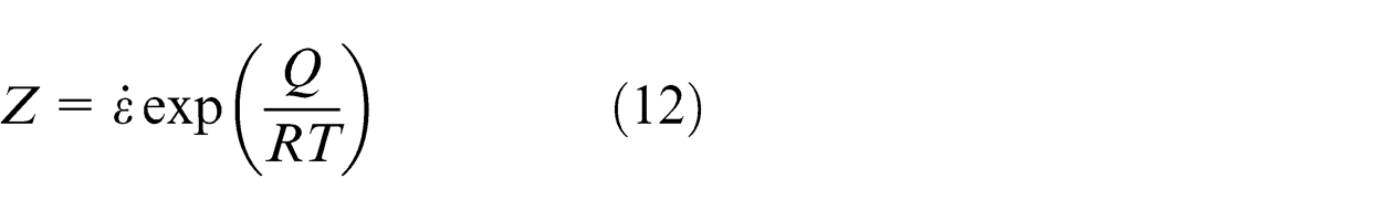
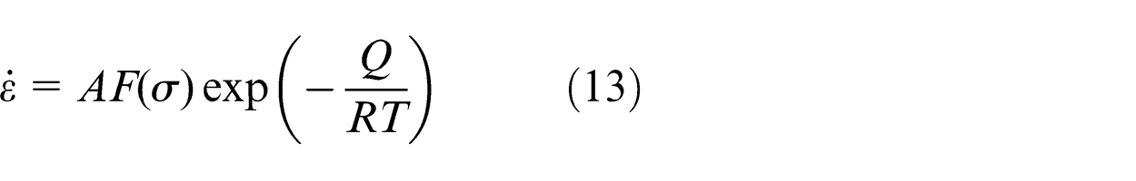
where
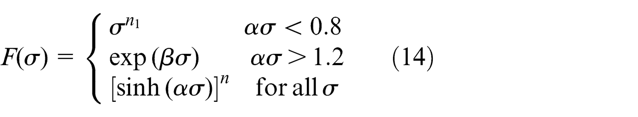
wherein
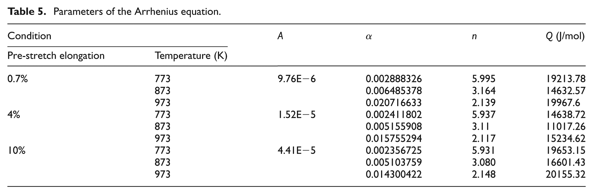
The parameters of the Arrhenius equation were fitted in ORIGIN and the results are given in Table 5.
Parameters of the Arrhenius equation.
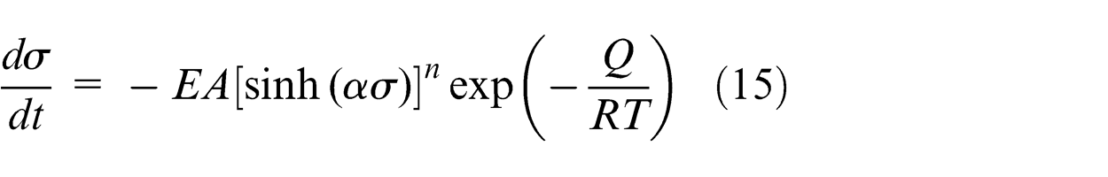
In order to calculate the deviation of the Arrhenius equation, the ordinary differential equation depends on equation (13) and can be expressed as
The fourth-grade fourth-order Runge–Kutta algorithm was employed to solve the ordinary differential equation. The iterative equations can be expressed as
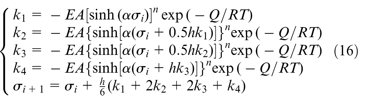
As the stability region for the fourth-grade fourth-order Runge–Kutta algorithm is
It can be seen from Figure 15 that the predicted stress–time curves agree well with the experimental data. The Arrhenius model can be considered effective to predict the flow stress behavior in the stress relaxation process.
FE simulation
The FE model of HSB was created in ABAQUS software. The geometrical model is shown in Figure 16. The jaw was connected to the part by tie constraint boundary condition.
Geometrical model for FE simulation.
The simulation of HSB could be divided into five steps: pre-stretch, bending, post-stretch, creep forming and springback. It is consistent with the deformation sequence of HSB experiment. The dwell time in creep forming was set as 0 (no stress relaxation process), 600 and 1200 s. A visco analysis step was employed to simulate the creep-forming process after the predefined field was loaded from the results of post-stretch. The springback process simulation was carried out by static general algorithm. The mesh size of profile is 5 mm in the length direction, 3 mm in the width direction and 1.5 mm in the rounded corner. The mesh type is set as Belytschko–Tsay shell element with five Gauss integral points in the sheet thickness direction. The constitutive equations in the stretch bending and creep-forming process were JC and Arrhenius equations with the parameters in Tables 3 and 5, respectively. Several parameters of the FE model are shown in Table 6.
Parameters in FE simulation of HSB.
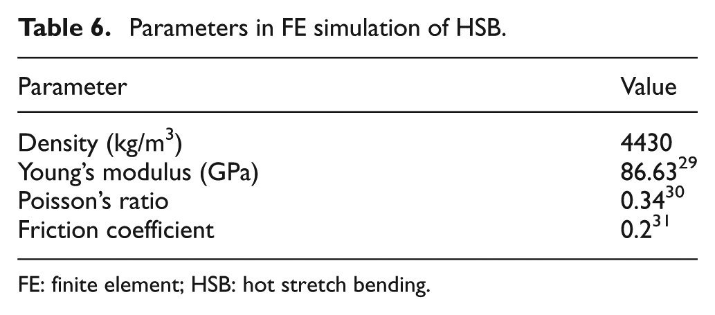
FE: finite element; HSB: hot stretch bending.
Results and discussion
It is found that the hot deformation behavior of Ti–6Al–4V alloy is related to the factors including strain rate, temperature and strain. The true stress–strain curves of uniaxial tensile tests show that the flow stress decreases with the increase in the temperature and decrease in the strain rate. At a given strain rate, the flow stress decreases as the temperature increases. However, at a given temperature, the flow stress increases as the strain rate increases. Each curve presents a peak stress in the flow curve at a particular strain and then follows a steady state.
The stress relaxation behavior is important to the analysis of the HSB process. Several characteristics of the stress relaxation can be obtained from the stress data of stress relaxation tests in Figure 14:
The stress relaxation can be divided into two stages qualitatively. In the first stage, the stress falls down rapidly. In the second stage, very slow relaxation occurs and the stress tends to arrive at a balance value gradually, which is called slack limit.
The temperature is the main parameter which controls the relaxation rate and slack limit. The higher the temperature, the lower the slack limit and the faster the relaxation rate the alloy can get.
The pre-stretch elongation has little effect on the relaxation process. However, the effect is indeterminate.
The stress distribution after the creep forming is shown in Figure 17.
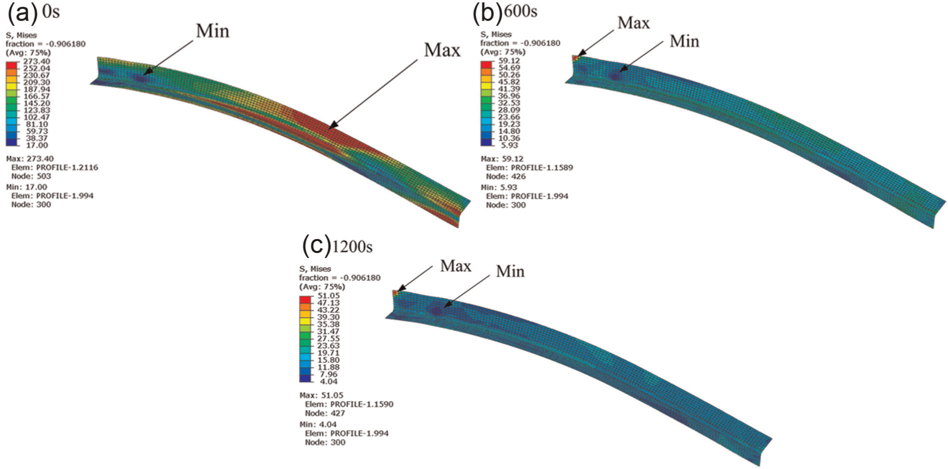
Stress distribution in the profile part during creep forming (MPa): (a) 0 s, (b) 600 s and (c) 1200 s.
Figure 17 indicates that the residual stress decreases sharply in the creep-forming stage. Meantime, distribution is more homogeneous. However, there is no large difference between 600 and 1200 s. This means the stress relaxation process of Ti–6Al–4V alloy at 973 K has basically completed in 600 s.
The gap, which represents the springback of the profile, is defined as the normal distance between the die and the profile part surface, as shown in Figure 18.
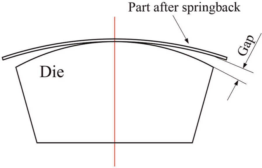
Gap definition after springback.
The gaps between the die surface and the profile in the experiment and FE simulation with different relaxation times are shown in Figure 19.
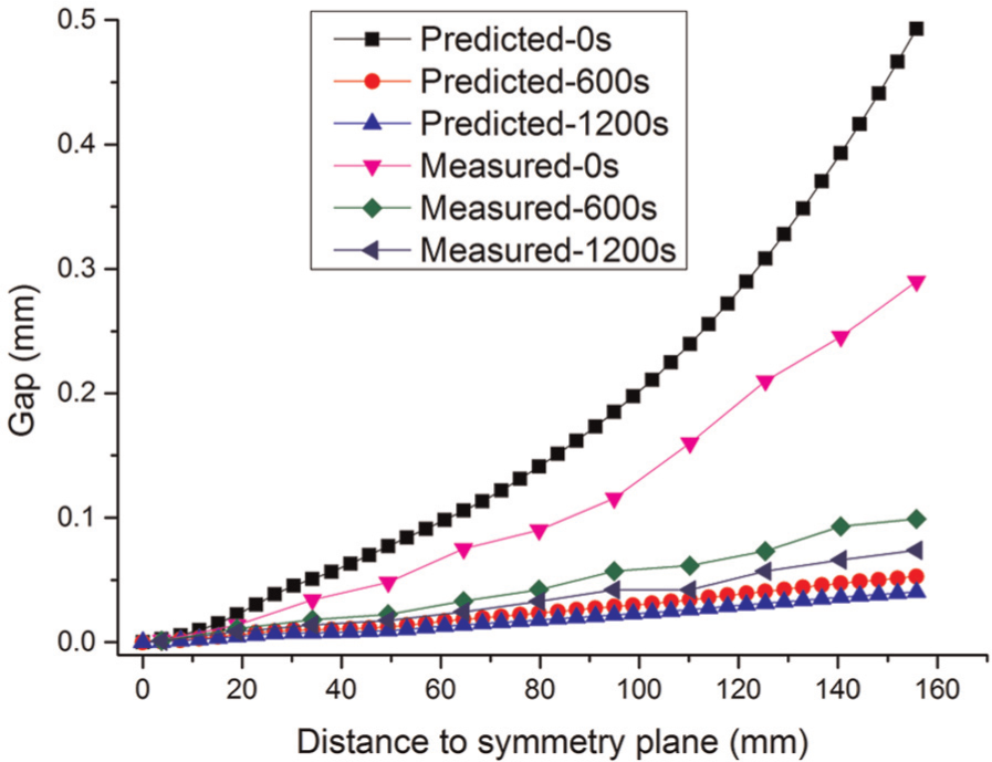
Gaps between surface of die and profile.
It can be seen from Figure 19 that the predicted springback shows promising agreement with the corresponding experimental observations. The FE model is applicable to satisfy the prediction of HSB process. Both the measured and predicted gaps decrease greatly after the creep process. The predicted gaps after 600 and 1200 s are very close to each other and far less than 0 s. This agrees well with the predicted residual stress. The measured gaps after 600 and 1200 s are larger than the predicted data. However, the opposite situation appears in 0 s (no relaxation). The reason can be attributed to the fact that the temperature of the profile cannot fall to room temperature immediately after stretch bending in the validation experiment; there is stress relaxation behavior in the cooling process.
Many efforts have been made to prevent the heat conduction between the part and the die. On one hand, the die was made of asbestos cement, which has a low thermal conductivity coefficient. On the other hand, before the HSB process, the die was pre-heated to the desired temperature by flame heating. However, there is still heat conduction between the profile part and the die during the HSB process. A temperature gradient exists in the cross section of the profile part. However, the thermocouple only measures the temperature in the upper portion of the profile rather than the lower portion. This could be the reason for the deviation between the FE simulation and the experimental ones.
Furthermore, the deviation between the FE simulation results and the experimental ones could be attributed to the fact that there is heat conduction between the profile part and the die. But the thermocouple measures the temperature in the upper portion of the profile rather than the lower portion. A temperature gradient exists in the cross section of the profile part.
This work has been limited to the material characterization and constitutive modeling of Ti–6Al–4V alloy based on the original JC model for the stretch bending stage. Considering the neglect of the coupled effects of strain rate–temperature–strain in the original JC model, modified models are necessary for numerical predictions with higher accuracy.
Conclusion
The material characterization and constitutive modeling of Ti–6Al–4V alloy in uniaxial tensile and stress relaxation are investigated to analyze the HSB process of the Ti–6Al–4V alloy profile in FE simulation. Furthermore, the validation experiment of the HSB process has been carried out. The main conclusions are summarized below:
The creep forming could be characterized by the stress relaxation behavior, which is mainly controlled by temperature and time. The higher the temperature, the lower the slack limit and the faster the relaxation rate the alloy can get.
The residual stress in the profile decreases greatly in the creep stage. Lower residual stress leads smaller springback in the HSB process. The predicted springback shows promising agreement with the corresponding experimental observations.
Footnotes
Declaration of Conflicting Interests
The author(s) declared no potential conflicts of interest with respect to the research, authorship, and/or publication of this article.
Funding
The author(s) disclosed receipt of the following financial support for the research, authorship, and/or publication of this article: The project was supported by State Key Laboratory of Materials Processing and Die & Mould Technology, Huazhong University of Science and Technology (P2014-003). Also, the authors are thankful to the sponsored items of the National Natural Science Foundation of China (51175022).