Sage Journals: Discover world-class research

Abstract

A jig-boring machine equipped with a dual-drive servo system can operate with high speed and accuracy. However, different friction behaviours and asymmetrical preloads of the double drive structures as well as asynchronous control over the master-slave motors can make the machine produce tremendous heat, causing uneven temperature distributions in the feed system and eventually leading to thermal deformation that reduces the positional accuracy of machines. To investigate the effects of thermal behaviours on machining accuracy, the thermal–structure finite element method was employed to analyse the transient thermal deformation and temperature field of the machine at different feed rates, considering boundary conditions such as the convective heat transfer coefficient and heat generation by motors, bearings, and screws. Additionally, a synchronous acquisition system was developed to measure the thermal behaviours, and the transient changes in temperature and deformation were compared with simulated values. Consequently, a synthetic thermal model was established to make accurate predictions based on the analysis of relationships between thermal error and equilibrium time, coordinate position and screw temperature. Finally, thermal error compensation was performed using a feedback integration method. The experimental data indicate that the finite element method model can accurately predict temperature distributions and thermal errors. Moreover, thermal errors were compensated at 24.1 °C and 22.6 °C with a feed rate of 18 m/min, and machining accuracy was increased by 73% and 62%, respectively.

Keywords

Boring machine finite element method temperature field thermal deformation compensation

Introduction

In modern machine tools, dual-drive servo feed systems have advantages such as high-speed feeds, good load-bearing capacity, and excellent acceleration/deceleration control, so they are widely used in large-scale precision boring machine designs. Machine tools equipped with a dual-drive servo system can achieve high speed and good accuracy. However, the dual-drive feed system is complex and causes many problems. For example, the heat generation by two friction pairs due to the screw and nut is different. Moreover, master-slave motor control and other processes are not synchronised, which causes the machine to release a large amount of thermal energy and hence affects machining accuracy. A dual-drive feed system can induce thermal error, which is a key factor limiting the precision and maintenance of computerised numerical control (CNC) machines. However, there are few published reports of the thermal error of jig-boring machines equipped with dual-drive servo systems. Moreover, although there is a thermal error compensation module in the Siemens CNC system, the absence of a systematic implementation scheme makes it difficult for users to master and apply the compensation technology.

The basic geometric accuracy of currently used Chinese precision boring machines is close to the international level, with linear positioning accuracy reaching 3 μm and repetitive positioning accuracy as high as 1.5 μm. However, the accuracy may decrease and become far lower than the initial design value after the machine is used for long-time periods. This decrease in accuracy over time primarily results from inadequate maintenance and unstable accuracy, and thermal error is the main factor leading to substandard accuracy, accounting for 70% of the total errors arising from various error sources.¹ Thermal error accounts for a larger proportion of total error as machine tools become more sophisticated. A non-uniform temperature distribution causes thermal errors in CNC machine tools, and the distribution becomes non-linear and non-stationary, varying with time. The mutual coupling of the location and intensity of the heat source, the thermal expansion coefficient and the machine structure create complex thermal characteristics.² Furthermore, the dynamical characteristics of the spindle also affect the thermal error. Zhang et al.³ proposed a holospectrum-based balancing method to improve the machining accuracy.

There are two methods to establish thermally induced error models that include experiments and simulations. The finite element method (FEM), used to analyse the temperature fields and thermal deformation of machine tools, has become a topic of increasing interest. Combining FEM simulations and experiments, Wu and Kung⁴ analysed the relationship between thermal deformation and preload, screw feed rate and the temperature field. Mian et al.⁵ also analysed thermal error and proposed an efficient prediction model. Min and Jiang⁶ presented a variety of thermal boundary conditions for a thermal error model based on the Fourier thermodynamic equation and analysed the gradient distribution of the screw temperature field under different heat fluxes. Won et al.⁷ used the modified lumped capacitance method and genius education algorithm to analyse the linear positioning error of the ball screw and estimated the thermal behaviour of the guideway by FEM. Kima et al.⁸ and Uhlmann and Hu⁹ investigated a linear-motor feed system and discussed how positioning accuracy was affected by the machine guideway and by the thermal deformation of linear encoders. The artificial neural network (ANN) was used to establish a relationship between temperature and the thermal error of a machine tool.^10–14 Although the ANN model was useful for making generalisations, its physical explanation was weak, and its predictive ability was heavily dependent on typical learning samples. Ramesh et al.¹⁵ developed a model using support vector machines that could effectively predict thermal errors.

Thermal error measurement is also important. Postlethwaite et al.¹⁶ made extensive use of thermal imaging for rapid assessment of machine tool thermal behaviour and off-line development of compensation models. Wang et al.¹⁷ introduced a new concept, in addition to the widely recognised error avoidance and error compensation approaches, to control the thermal effects during machining by monitoring the thermal status of the machine.

If thermal errors can be measured and modelled, the next step is to compensate them. There are many scholars studying this issue who have made numerous scientific achievements, including Pahk and Lee,¹⁸ Postlethwaite et al.,¹⁹ Yang and Ni,²⁰ Du et al.,²¹ and Li and Zhao.²² Gebhardt et al.²³ described a high-precision grey-box model for the compensation of thermal errors on a five-axis machine and reduced the thermally induced errors in rotary/swivelling by up to 85%. Pajor and Zapata²⁴ presented a set of approaches allowing the supervision of feed screw thermal elongation to reduce thermal errors. Miao et al.²⁵ built an axial thermal error model of the spindle using a multivariate linear regression method. Wang and Yang²⁶ also proposed a prediction model for axial thermal deformation and applied the model to compensate a CNC machine. Zhang et al.²⁷ proposed a compensation technique based on machine zero point shift and wrote an Ethernet data communication protocol for machine tools, improving machine precision.

At present, few reports in the literature have been concerned with transient simulation of the thermal behaviours of machine tools equipped with double drive servo feed systems. In addition, no experiments have been conducted in which the thermal deformation and temperature fields of motors, bearings, screws, and other parts of the machine tools are simultaneously measured. Moreover, while there have been many studies about thermal error compensation of motorised spindles, studies about feed systems are relatively rare. Furthermore, the thermal error compensation methods in published reports have mainly been based on the origin offset principle of the machine, which places high demands on the interface between the CNC system and the computer used for thermal error compensation. Thus, this method is not easy to implement in industrial applications. Finally, although there is a thermal error compensation module in the Siemens CNC system, the absence of a systematic implementation scheme makes it difficult for users to master and apply the compensation technology.

This article proposes a systematic method to analyse the thermal characteristics of a jig-boring machine equipped with a dual-drive servo feed system. A thermal–structure FEM model for the machine is presented; it considers boundary conditions such as the convection heat transfer coefficient and heat generation by the motors, bearings, and screw. Next, the transient thermal deformation and temperature distribution of the feed system were analysed at different feed rates. A synchronous acquisition system was then developed to measure the temperature and thermal deformation, and the measured and simulated results were in very good agreement. Subsequently, a synthetic thermal model with accurate prediction was established, based on the analysis of relationships between the thermal error and thermal equilibrium time, coordinate position, and the typical characteristic temperature of the screw. Finally, the thermal error compensation module was developed, and error compensation was conducted using the feedback integration method. Accordingly, a systematic solution was described to investigate the compensation technique of thermally induced error, which effectively improved the accuracy of the machine and could be useful in industrial applications.

Thermal behaviour simulation

FEM

In this article, we focus on a precision CNC jig-boring machine tool. The system analyses the change in the temperature field and the thermal deformation of the feed system. The positioning accuracy of the machine is 3 μm, and the repetitive positioning accuracy is 1.5 μm. The three axes have a synchronous dual-drive architecture with a travel range of 1200 × 1000 × 1000 mm and a maximum point-to-point feed rate of F = 64 m/min; the actual processing maximum feed rate is F = 45 m/min, and the screw has an internal cooling structure. The thermal behaviours for the X-axis were simulated at feed rates of 6, 12, 18 and 24 m/min.

The research object in this study is a large-scale jig-boring machine with a complex structure and numerous parts. If the machine structure is not reasonably simplified, it is difficult to generate mesh and load boundary conditions, leading to poor convergence of results and overly long solution times. In addition, the accuracy of the simulated results may not be higher with the original structure than with a simplified structure. To obtain a good balance between calculation efficiency and simulation accuracy, the entity model should be reasonably simplified, and structures that have less influence on the simulation results, such as such as bolt holes, chamfers, fillets, and small reinforcing plates, should be removed.

Moreover, the motors are equivalent to cylinders with constant heat rations. The screws are equivalent to cylinders with smooth surfaces, and the bearings are equivalent to rings.

Different types of elements are used to mesh every part of the three-dimensional (3D) model of the machine tool. Meanwhile, a complex component can be meshed by applying many different types of elements, as there is no causal relationship between the parts and the mesh elements. The meshed model is shown in Figure 1(a)–(b), and the specific parameters of the mesh elements are shown in Table 1. The elements between the contact units are not easily displayed and are marked with the red and blue colours.

Figure 1.

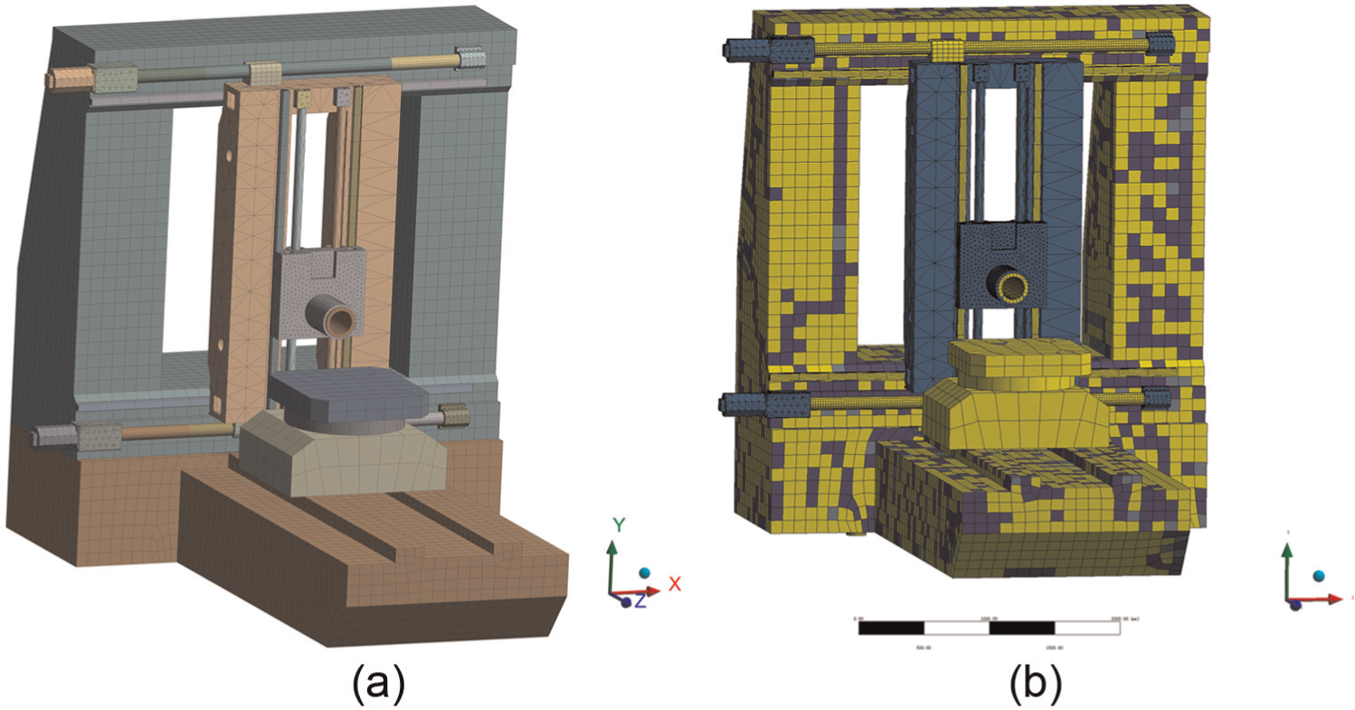
(a) mesh of the machine tool (b) element type of the machine tool

Table 1.

Element types in the boring machine mesh.

Generic element type name	Mechanical APDL name	Type	Colour
Quadratic tetrahedron	Solid87	3D 10-node tetrahedral thermal solid	Dark blue
Quadratic hexahedron	Solid90	3D 20-node thermal solid	Yellow
Quadratic wedge	Solid90	3D 20-node thermal solid	Grey
Quadratic pyramid	Solid90	3D 20-node thermal solid	Purple
Quadratic quadrilateral contact	Conta174	3D 8-node surface-to-surface contact	Red
Quadratic quadrilateral target	Targe170	3D target segment	Blue
Quadratic triangular contact	Conta174	3D 8-node surface-to-surface contact	Red
Quadratic triangular target	Targe170	3D target segment	Blue

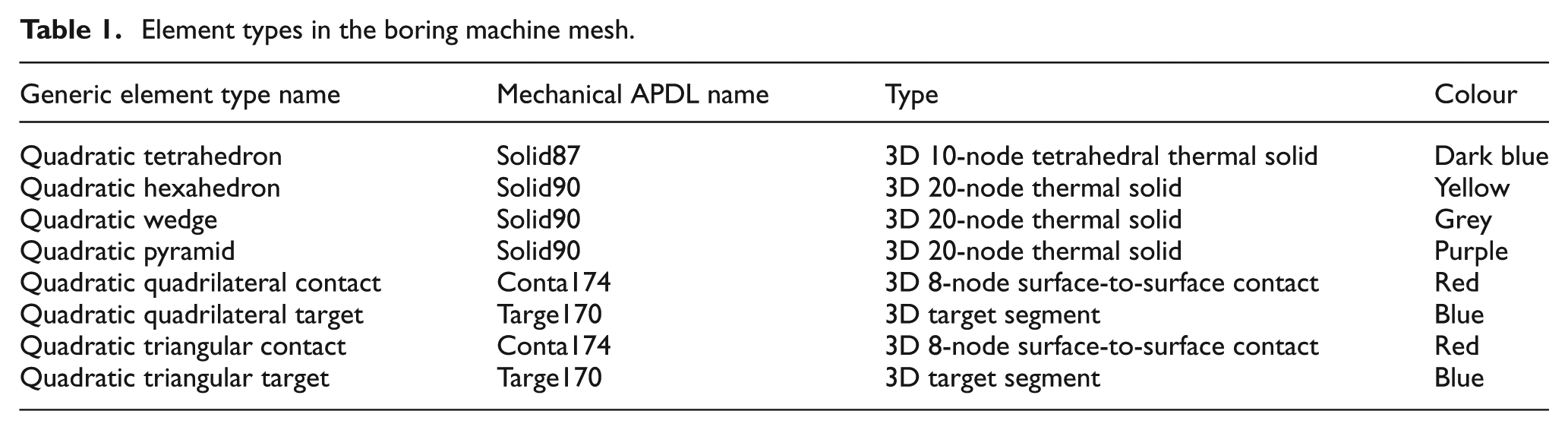
The FEM of the jig-boring machine was conducted with the ANSYS workbench module. The transient thermal–structural coupling was analysed, and the transient thermal deformation was simulated with heat as the input. There is a total of 401,004 nodes and 164,758 elements in the model. The elements used in the FEM model are shown in Table 1. SOLID90 is a 3D 20-node solid thermal element. The element has 20 nodes with a single degree of freedom, namely temperature, at each node. The 20-node elements have compatible temperature shapes and are well suited to model curved boundaries. The 20-node thermal element is applicable to a 3D, steady-state or transient thermal analysis. SOLID87 is a 3D 10-node tetrahedral thermal solid element that is applicable to steady-state or transient thermal analysis and that is well suited to model irregular meshes. The element has 1 degree of freedom, namely temperature, at each node. CONTA174 is 3D 8-node surface-to-surface contact element, and it is used to represent contact and sliding between 3D ‘target’ surfaces (TARGE170) and a deformable surface defined by this element. This element is located on the surfaces of 3D solid or shell elements with midsize nodes. Coulomb and shear stress friction is allowed. TARGE170 is a 3D target segment element that is associated with a contact surface via a shared real constant set. The contact elements themselves overlay the solid, shell or line elements describing the boundary of a deformable body and are potentially in contact with the target surface, defined by TARGE170.

Based on the heat conduction equation, the transient heat transfer model is defined as^9,28

Q = ρ C_{p} \partial T / \partial t + \nabla^{T} q

(1)

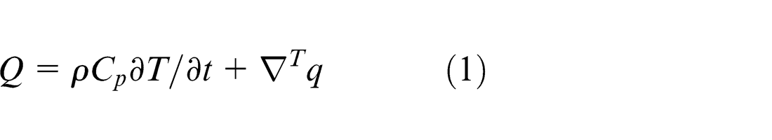
where Q is the power density, $ρ$ is the mass density, C_p is the specific heat capacity, T is the temperature distribution in space and time, $\nabla$ is the gradient operator and q is the heat conductivity.

The jig-boring machine deformation induced by thermal expansion can be calculated through load–deformation analysis. The strain vector $ε$ can be determined by Hooke’s law

ε = α \cdot Δ T

(2)

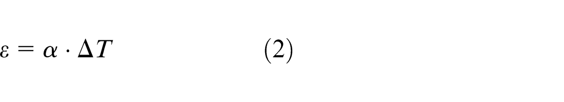
where $α$ is the thermal expansion coefficient and $Δ T$ is the temperature variation.

The main heat source of a ball screw system is the friction caused by a moving nut and the support bearings. Some assumptions are made to perform the thermal analysis by FEM:

The simulation is performed under the air cutting condition, and thus, the cutting heat and its effects are not considered.

The screw shaft is a solid cylinder.

Heat radiation to the surrounding environment is ignored.

The temperature-dependent non-linear properties of the material (thermal conductivity, heat capacity, thermal expansion and so on) are not considered because the ambient temperature is 20 °C.

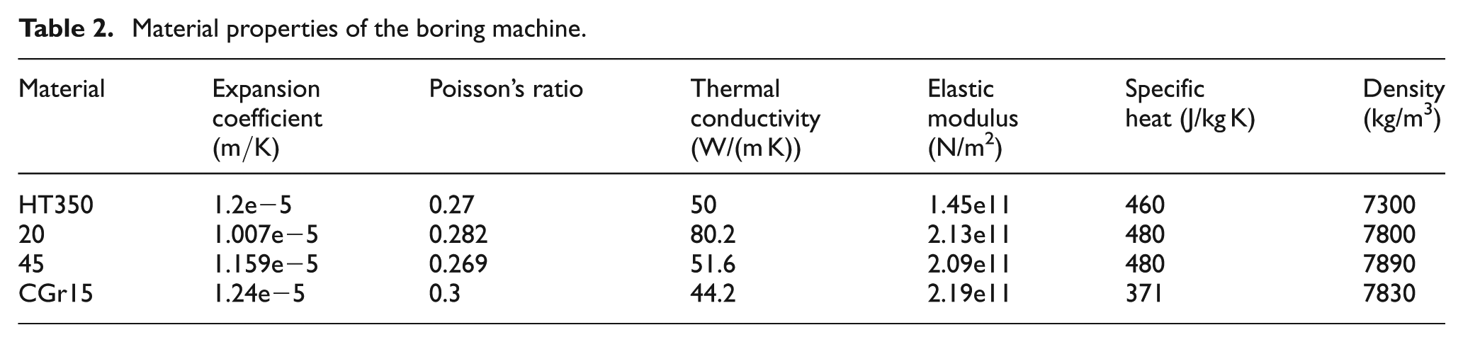
The material features of the machine, such as density, specific heat capacity, thermal conductivity, coefficient of expansion, elastic modulus, shear modulus, and Poisson’s ratio, are considered in the FEM model and described in Table 2.

Table 2.

Material properties of the boring machine.

Material	Expansion coefficient ( $m / K$ )	Poisson’s ratio	Thermal conductivity (W/(m K))	Elastic modulus (N/m²)	Specific heat (J/kg K)	Density (kg/m³)
HT350	1.2e−5	0.27	50	1.45e11	460	7300
20	1.007e−5	0.282	80.2	2.13e11	480	7800
45	1.159e−5	0.269	51.6	2.09e11	480	7890
CGr15	1.24e−5	0.3	44.2	2.19e11	371	7830

Heat transfer coefficient

In the FEM model, the heat transfer coefficient $α$ describing convection was given by Frank and Incropera²⁹

α = \frac{Nu \cdot λ}{h_{g}}

(3)

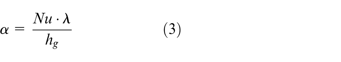
where Nu is the Nusselt number, $λ$ is the fluid thermal conductivity and h_g is the characteristic length. For natural convection, Nu is a function of the Reynolds number Re and Prandtl number Pr, and the flowing state of the fluid is determined by the Reynolds number Re

Re = \frac{\bar{u} \cdot h_{g}}{v}

(4)

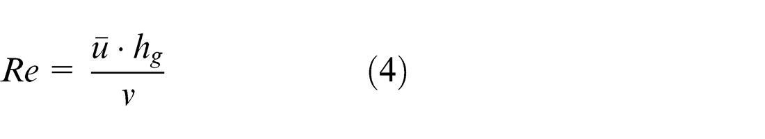
where Re determines the flowing state of the coolant, $\bar{u}$ is the average velocity of the fluid and $v$ is the kinematic viscosity of the fluid.

The Prandtl number Pr is determined by the materials of the machine

\Pr = \frac{c \cdot μ}{λ}

(5)

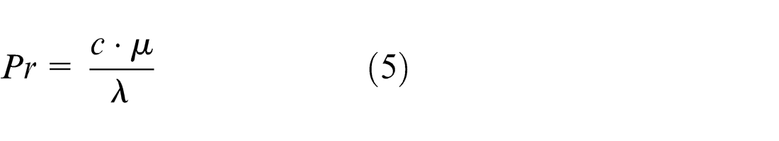
where c is the fluid capacity and $μ$ is the fluid dynamic viscosity.

Nu can be determined by applying equations (4) and (5)

Nu = 0.0225 \cdot {Re}^{0.8} \cdot \Pr^{N}

(6)

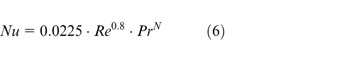
where the N is a constant.

The computed results show that the forced convective heat transfer coefficient of the cooling fluid is 4300 W/m² k, and the natural air convection heat transfer coefficient is 9.7 W/m² k. The ambient temperature is 20 °C.

Power calculation of the heat sources

Computation of the screw thermal generation

We assume that the frictional heat generated between the moving nut and the screw shaft is uniform at the contacting surfaces and is proportional to the time, and that heat generation at support bearings is a constant.

The heat $Q$ generated by the screw shaft can be defined as³⁰

Q = \frac{nM}{9550}

(7)

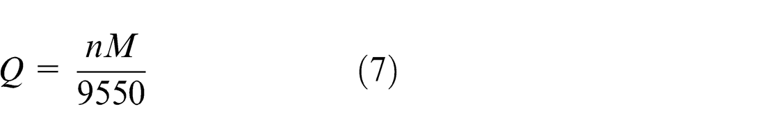
where n is the rotation rate of the nut and M is the total frictional torque.

If the axial load of the screw is F_a , the torque M ₁ required to drive the nut is

M_{1} = \frac{F_{a} P_{h}}{2 π η}

(8)

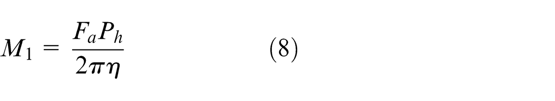
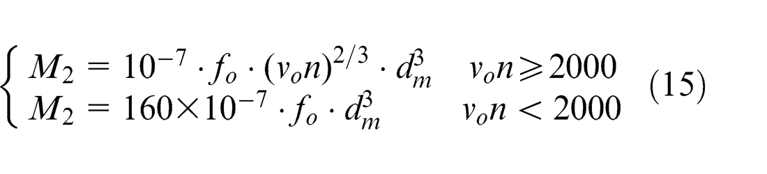
where $P_{h}$ is the screw input power and $η$ is the nut efficiency of the ball screw.

The ball screw resistance moment M ₂ is obtained by

M_{2} = \frac{F_{a} P_{h}}{2 π η} (1 - η^{2})

(9)

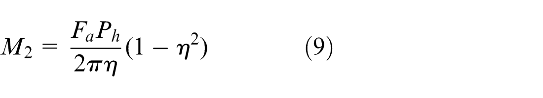
The total frictional torque M can be approximated as

M = 0.94 M_{2} + M_{1}

(10)

The calculated result indicates that the screw heat power is 262w.

Bearing thermal generation model

Harris noted that heat generation by the bearing is mainly due to the external loads and the viscous friction of the lubricant. In addition, the rolling body spin motion in the raceway also generated heat due to frictional torque. The dominant heat is generated by bearings causing thermal deformations. The heat can be calculated by the following equation^30–32

Q_{total} = 1.047 \times 10^{- 4} \times n \times M

(11)

where Q_total is the heat generated by the bearing (w), n is the rotation rate of the bearing (r/min) and M is the total frictional torque (N mm). The frictional torque M consists of two components: one is caused by the applied load M ₁ and the other by the viscosity of the lubricant M ₂

M = M_{1} + M_{2}

(12)

The applied load M ₁ can be given by the following equation^31,33

M_{1} = f_{1} \cdot F_{β} \cdot d_{m}

(13)

F_{β} = max (0.9 F_{a} / \tan α - 0.1 F_{r}, F_{r})

(14)

where $f_{1}$ is a quotient related to the bearing type, $F_{β}$ is the bearing load (N), and d_m is the mean diameter of the bearing (mm). $F_{a}$ and $F_{r}$ are axial and radial forces, respectively. The viscosity of the lubricant M ₂ can be computed by equation (15)

{\begin{matrix} M_{2} = 10^{- 7} \cdot f_{o} \cdot {(v_{o} n)}^{2 / 3} \cdot d_{m}^{3} v_{o} n \geq 2000 \\ M_{2} = 160 \times 10^{- 7} \cdot f_{o} \cdot d_{m}^{3} v_{o} n < 2000 \end{matrix}

(15)

where f_o is a factor related to bearing type and lubrication method and v_o is the kinematic viscosity of the lubricant (mm²/s). The bearing heat power is 605w.

Motor heat generation model

The motor power losses can be obtained by calculating the motor efficiency³⁴

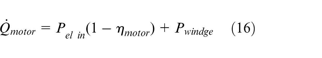
{\overset{\cdot}{Q}}_{motor} = P_{el \begin{matrix}  \end{matrix} in} (1 - η_{motor}) + P_{windge}

(16)

where ${\overset{\cdot}{Q}}_{motor}$ is the heat generated by the motor (w), $P_{el \begin{matrix} \end{matrix} in}$ is the motor input power, $η_{motor}$ is the motor efficiency, and $P_{windge}$ is the motor wind losses.

Motor power loss allocation between the rotor and the stator is determined by the motor slip and synchronous frequency, and the analytic expression is as follows

{\begin{matrix} {\overset{\cdot}{Q}}_{rotor} = {\overset{\cdot}{Q}}_{motor} \cdot \frac{f_{slip}}{f_{sync}} \\ {\overset{\cdot}{Q}}_{stator} = {\overset{\cdot}{Q}}_{motor} - {\overset{\cdot}{Q}}_{rotor} \end{matrix}

(17)

where ${\overset{\cdot}{Q}}_{rotor}$ is the rotor-generated heat, ${\overset{\cdot}{Q}}_{stator}$ is the stator-generated heat, f_slip is the slip frequency, and f_sync is the synchronous frequency (Hz). The calculation results show that the motor power is 20 kW, and its total heat power is 2500 W; the stator heat power is 1650 W and the rotor heat power is 850 W.

Transient simulation analysis

As an example, the simulation results were analysed at a feed rate of F = 18 m/min. The thermal balance experiments were performed in an enthalpy chamber at 20 °C, and the simulation reference temperature was set to 20 °C. The contact resistance was 8650 m² k/W.

Temperature field characteristics

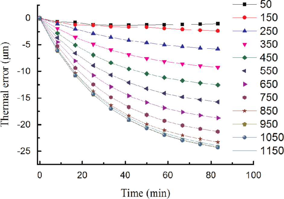
The simulated temperature distribution at t = 83 min is shown in Figure 2. For the X-axis dual-drive structure, the temperature of the upper motor is significantly higher than that of the lower motor, and the temperatures of the upper front and rear bearings are also higher than those of the lower bearings due to the friction between the screw and nut caused by the asynchrony of the upper and lower motors. In addition, the power and load of the upper motor, the active end of the dual-drive system, are larger and thus generate a larger amount of heat, resulting in temperature increases. The temperature of the upper motor can reach 40.2 °C in the equilibrium state, which is higher than that of the front (29.8 °C) and rear bearings (20.8 °C) in the upper drive system. The temperature of the lower motor is also higher than that of the front and rear bearings in the lower drive system, whose thermal equilibrium temperature is 36.7 °C. Therefore, the uneven temperature gradient distribution is caused by the temperature differences among the screw and the motors and bearings of the upper and lower drive feed systems. The uneven distribution leads to thermal deformation and degradation of the positioning and repetitive positioning accuracy; the thermal deformation can be used to guide the thermal balance design of a precise jig-boring machine. The screw temperatures in the range [−50 mm, −1,150 mm] are significantly higher than that of the other stroke, and the simulated maximum temperature is 24.6 °C at thermal equilibrium. Figure 3 shows the transient simulated temperature distribution of the screw.

Figure 2.

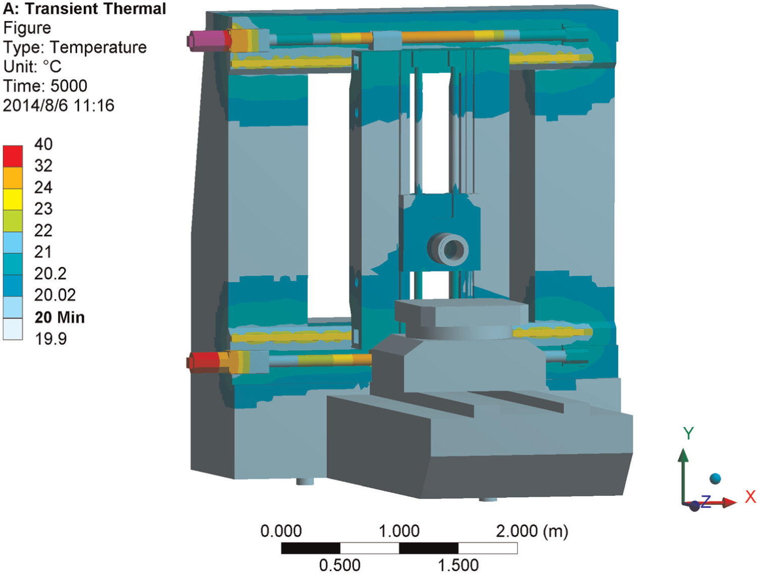
Temperature distribution of the boring machine.

Figure 3.

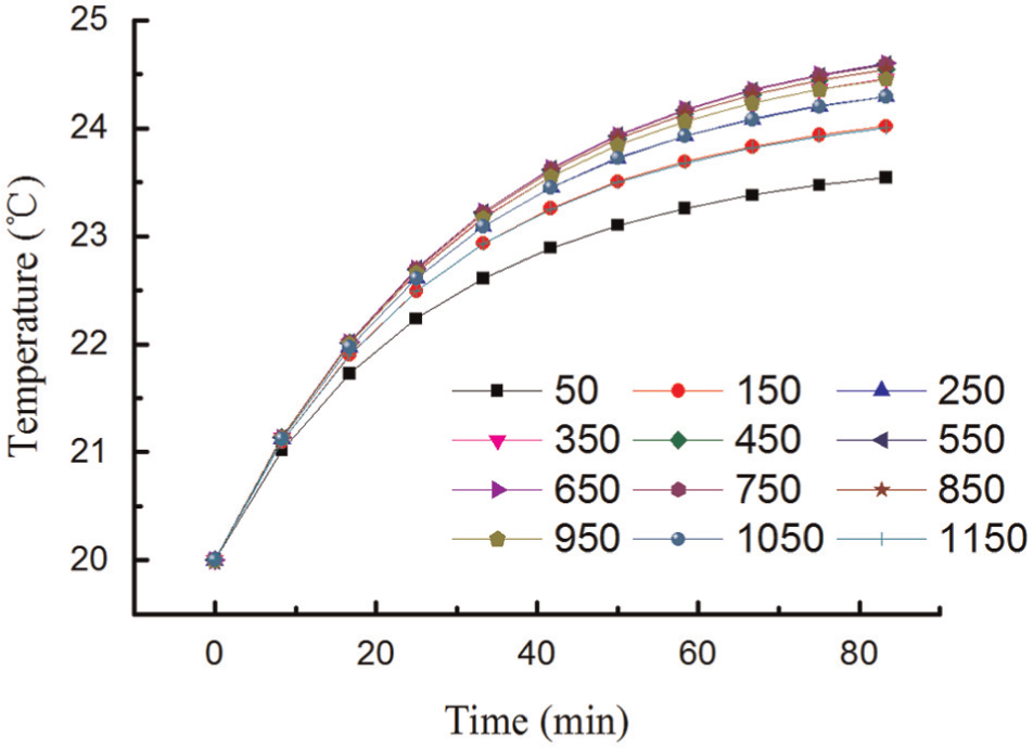
Simulated temperatures of the upper screw.

Thermal deformation of the feed system

The deformation of the screw shaft and scale under running conditions is one of the important factors leading to the degradation of positioning accuracy. The simulation results show that the X-axis scale has a large thermal deformation, as shown in Figure 4. Figure 5 shows that the heat distortion values of the 12 measuring points on the scale increase with time. The maximum thermal deformation of the scale is −24.3 μm at X = −1050 mm, while the maximum thermal expansion of the screw reaches 17.8 μm. This result shows that the thermal deformation of the scale is the main factor reducing positioning accuracy.

Figure 4.

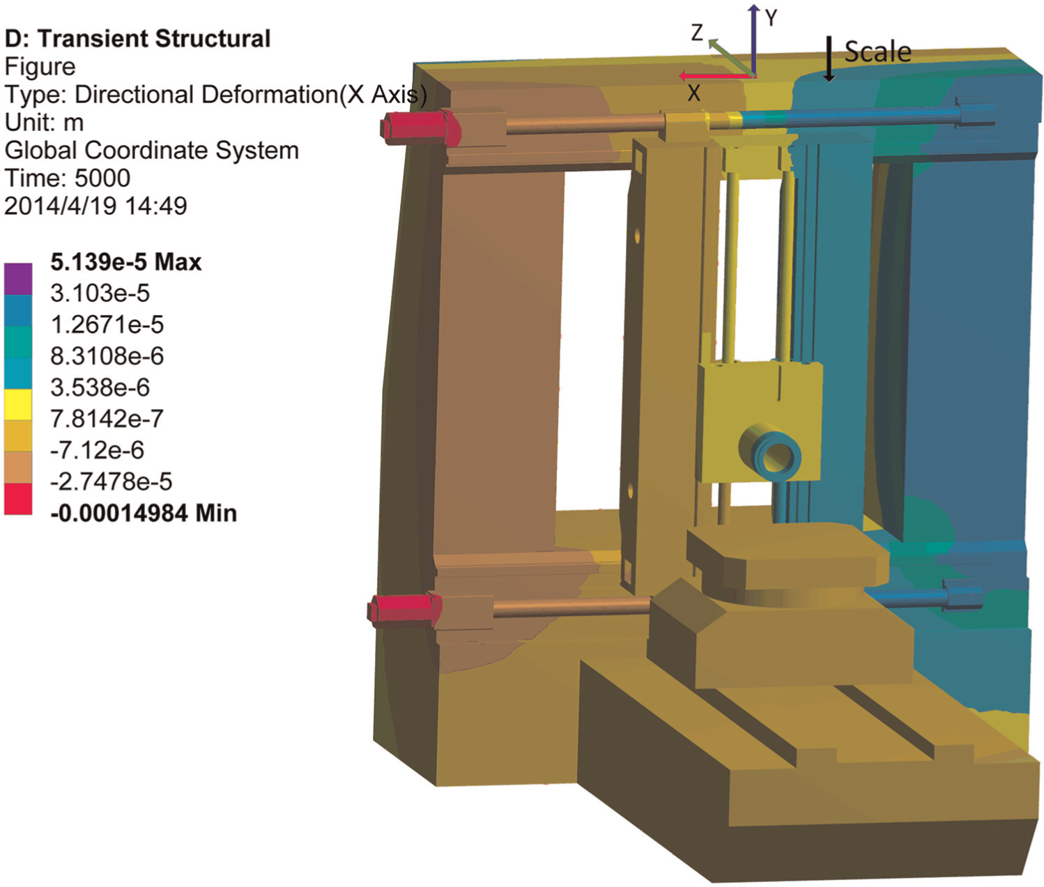
Deformation distribution of the boring machine.

Figure 5.

Simulated deformation of the scale in the X direction.

Experimental verification

Experimental system

The experimental measurement setup is shown in Figure 6(a); it consists of a Renishaw XL80 laser interferometer used to obtain the position-dependent thermal error of the feed system; a FLIR SC7000 infrared camera used to measure the XY plane temperature field and a synchronous acquisition system (developed by our group with an NI-SCXI as its structural base) used to determine the temperature and thermal deformation. PT100 precision temperature sensors are used to measure the temperature for the feed system motors, bearings, nut seat, guideway, and environment in the system. A high-precision eddy-current sensor was employed to measure the screw terminal thermal expansion. These three systems shown in Figure 6(b) collect data synchronously.

Figure 6.

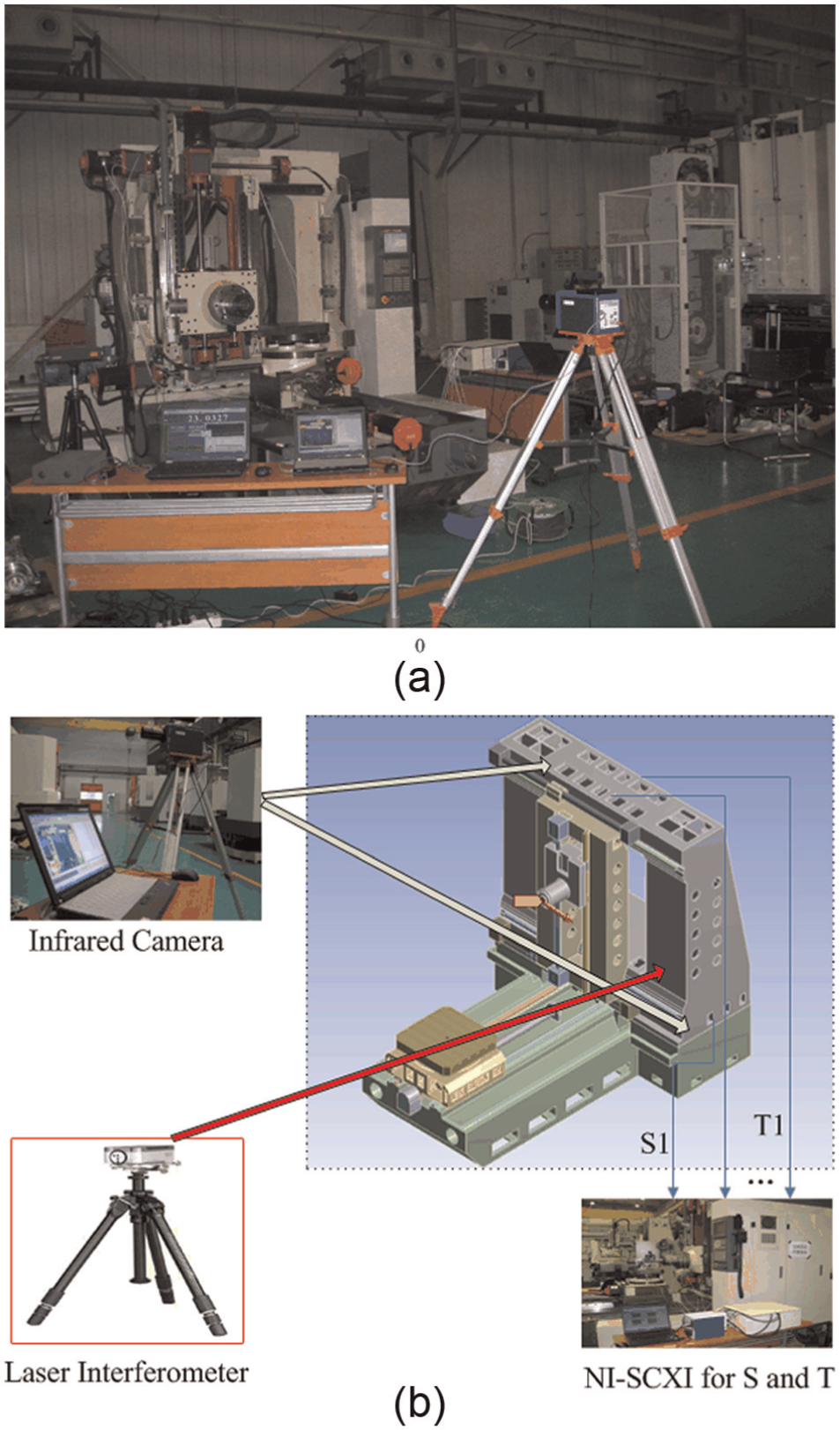
(a) Experimental setup and (b) schematic diagram of the measurement system.

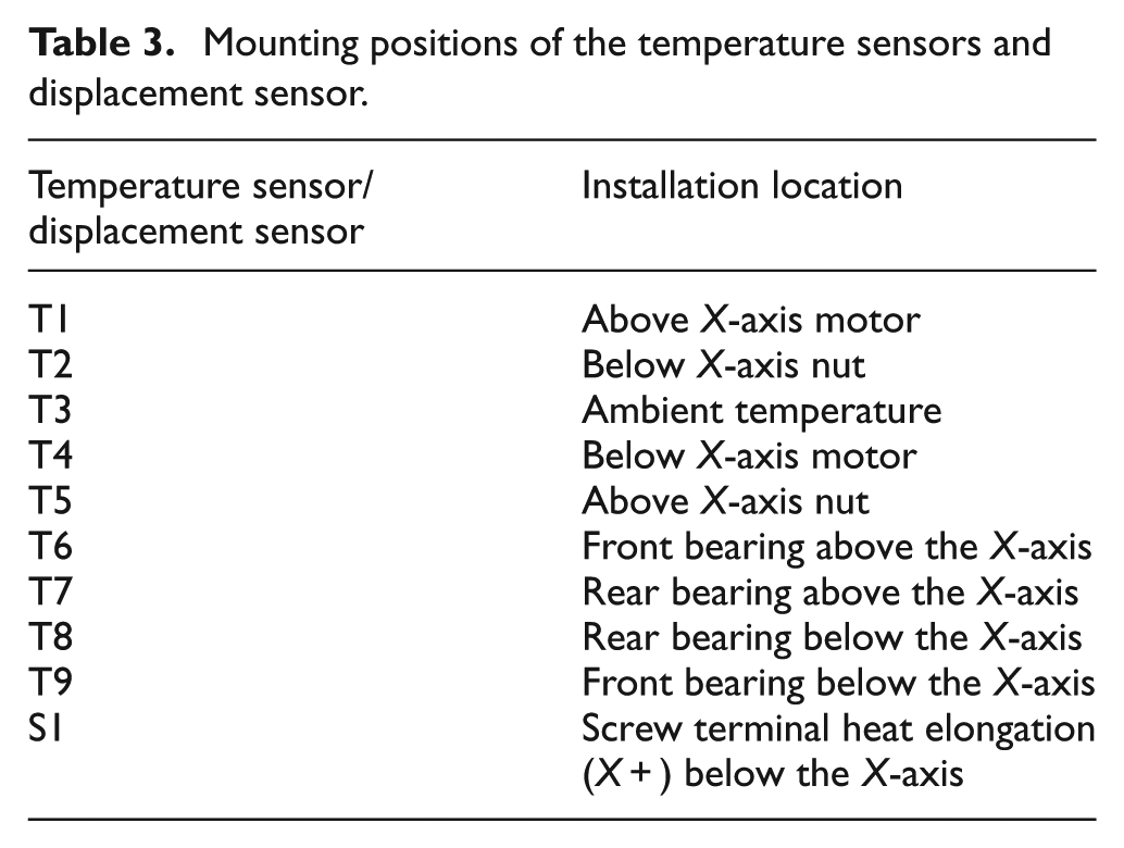
The mounted positions of the magnetic temperature sensors (PT100) in the machine are described in Figure 7 and Table 3 and are denoted as T1–T9. S1 is the eddy-current displacement sensor.

Figure 7.

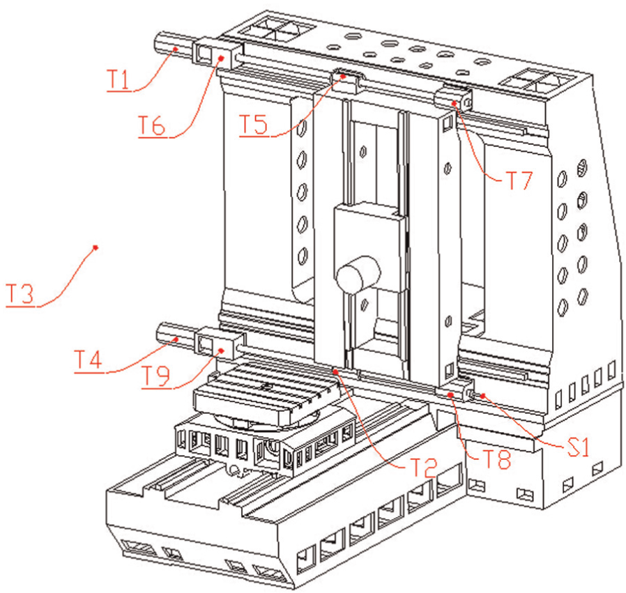
Mounting positions of sensors on the machine tool.

Table 3.

Mounting positions of the temperature sensors and displacement sensor.

Temperature sensor/displacement sensor	Installation location
T1	Above X-axis motor
T2	Below X-axis nut
T3	Ambient temperature
T4	Below X-axis motor
T5	Above X-axis nut
T6	Front bearing above the X-axis
T7	Rear bearing above the X-axis
T8	Rear bearing below the X-axis
T9	Front bearing below the X-axis
S1	Screw terminal heat elongation (X+) below the X-axis

Measurement principle

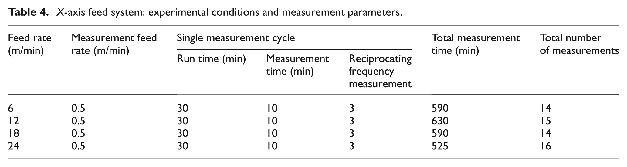
As shown in Table 4, the thermal behaviours of the X-axis were measured at four feed rates at a constant temperature of 20 °C. The distribution of the measured points along the feed axis is shown in Figure 8, and the range of points was [−50 mm, −1,150 mm] with an even interval of 100 mm. There are 12 measurement points, and the coordinate P0 is denoted as the origin of the laser interferometer.

Table 4.

X-axis feed system: experimental conditions and measurement parameters.

Feed rate (m/min)	Measurement feed rate (m/min)	Single measurement cycle			Total measurement time (min)	Total number of measurements
Feed rate (m/min)	Measurement feed rate (m/min)	Run time (min)	Measurement time (min)	Reciprocating frequency measurement	Total measurement time (min)	Total number of measurements
6	0.5	30	10	3	590	14
12	0.5	30	10	3	630	15
18	0.5	30	10	3	590	14
24	0.5	30	10	3	525	16

Figure 8.

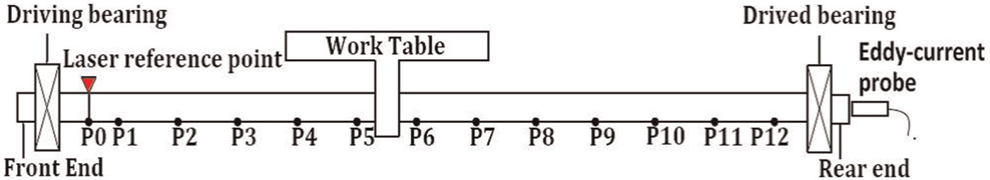
Distribution diagram of the measured points on the feed axis.

The errors at each point were measured in the cold state before the feed system was operated continually; these were marked as geometric errors. The feed axis was continuously run back and forth at each feed rate. Data were collected every 30 min, and thermal errors were recorded, defined as the collected data minus the geometric error.²² To avoid the influence of heat on the measurement results at high rates, we limited the feed rate to F = 0.5 m/min. According to the standards of VDI and ISO, each measurement undergoes three reciprocating cycles, and it takes 2 s for the laser interferometer to complete the measurement at each point. At each measurement point, the machine was suspended for 5 s. The reverse overrun was set at 2 mm to prevent measurement error caused by backlash.

The measurement points are denoted as i = 1, 2,..., 12, the number of measurements is denoted by j = 1, 2,..., N, and the number of feed axis reciprocating cycles in a single measurement is k = 1, 2,..., 6. $E_{ij}^{k}$ denotes the thermal error of the No. i measurement point of the screw at the jth measurement measured by the three reciprocating cycles of the kth measurement value. E _i0 is the geometric error of the ith point of the screw in the cold state

E_{i 0} = \frac{1}{6} \sum_{k = 1}^{6} E_{i 0}^{k}

(18)

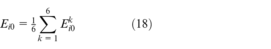
The ith measurement point of the jth measured thermal error is

Δ E_{ij} = \frac{1}{6} \sum_{k = 1}^{6} (E_{ij}^{k} - E_{i 0}^{k})

(19)

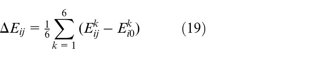
Assuming that T_ij is the ith measurement point of the jth measured temperature using the infrared camera, T_j is the screw characteristic temperature at the jth measurement

T_{j} = \frac{1}{12} \sum_{i = 1}^{12} T_{ij}

(20)

The terminal thermal elongation of the lower screw, along with ambient temperature and the temperatures of the upper and lower motors, front and rear bearings, and nut seat, was collected synchronously each second by the acquisition system.

Results and analysis

The thermal error of a precision CNC machine tool results from many complex factors, such as the processing method, material type, processing path, ambient temperature, cooling systems, cutting fluids, cutting parameters, screw preload, and, in particular, the key factor of feed rate. In this article, the thermal characteristics of the machine were analysed based on experiments at different feed rates. In addition, because thermal behaviours are sensitive to temperature, the test was performed in an enthalpy chamber at 20 °C. To verify the thermal FEM model, the temperature of key points and the thermal deformation were extracted and compared with the measured value.

Comparison of the simulated and the measured temperature

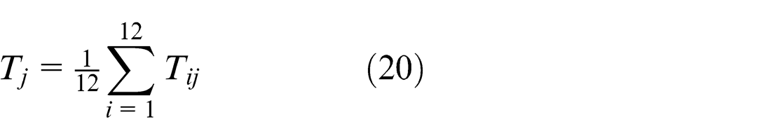
Figures 9 and 10 show comparisons between the simulated and the measured temperatures of the motors and bearings in the X-axis at 6, 12, 18, and 24 m/min. The overall trends of the simulated temperatures are similar to the measured temperatures, and they increase as the feed rate increases. Furthermore, the temperatures of the upper motor and bearing are higher than those of the lower. However, the thermal equilibrium time of the simulation is 83 min, which is much lower than the measured value of 525 min. There are two primary reasons for this discrepancy. First, in the simulation, the simplified machine structure and exclusion of complex boundary conditions, such as radiation and thermal resistance between the complex structural parts, could shorten the heat transfer process and reduce the thermal equilibrium time. In addition, the feed rate during the measurement was far less than that during the running process, so the loss of heat during the measurement also increased the thermal equilibrium time.

Figure 9.

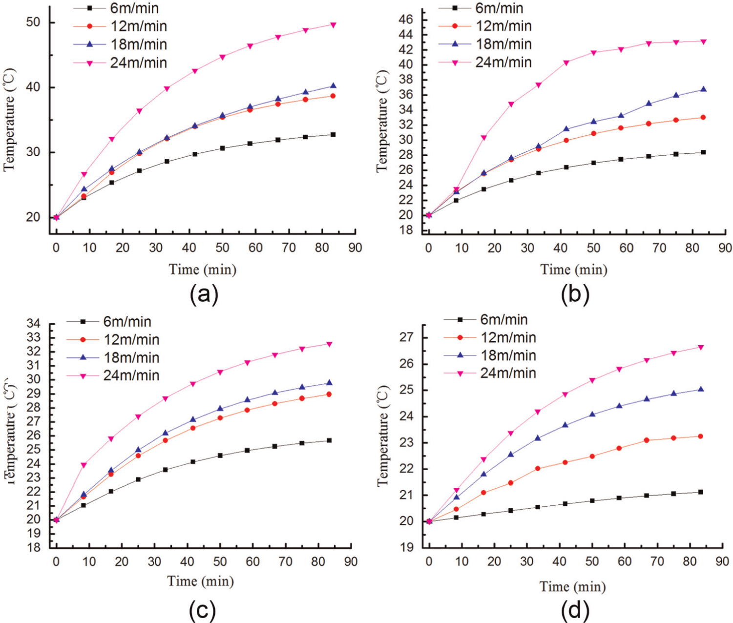
Simulated temperatures: (a) upper motor, (b) lower motor, (c) upper bearing, and (d) lower bearing.

Figure 10.

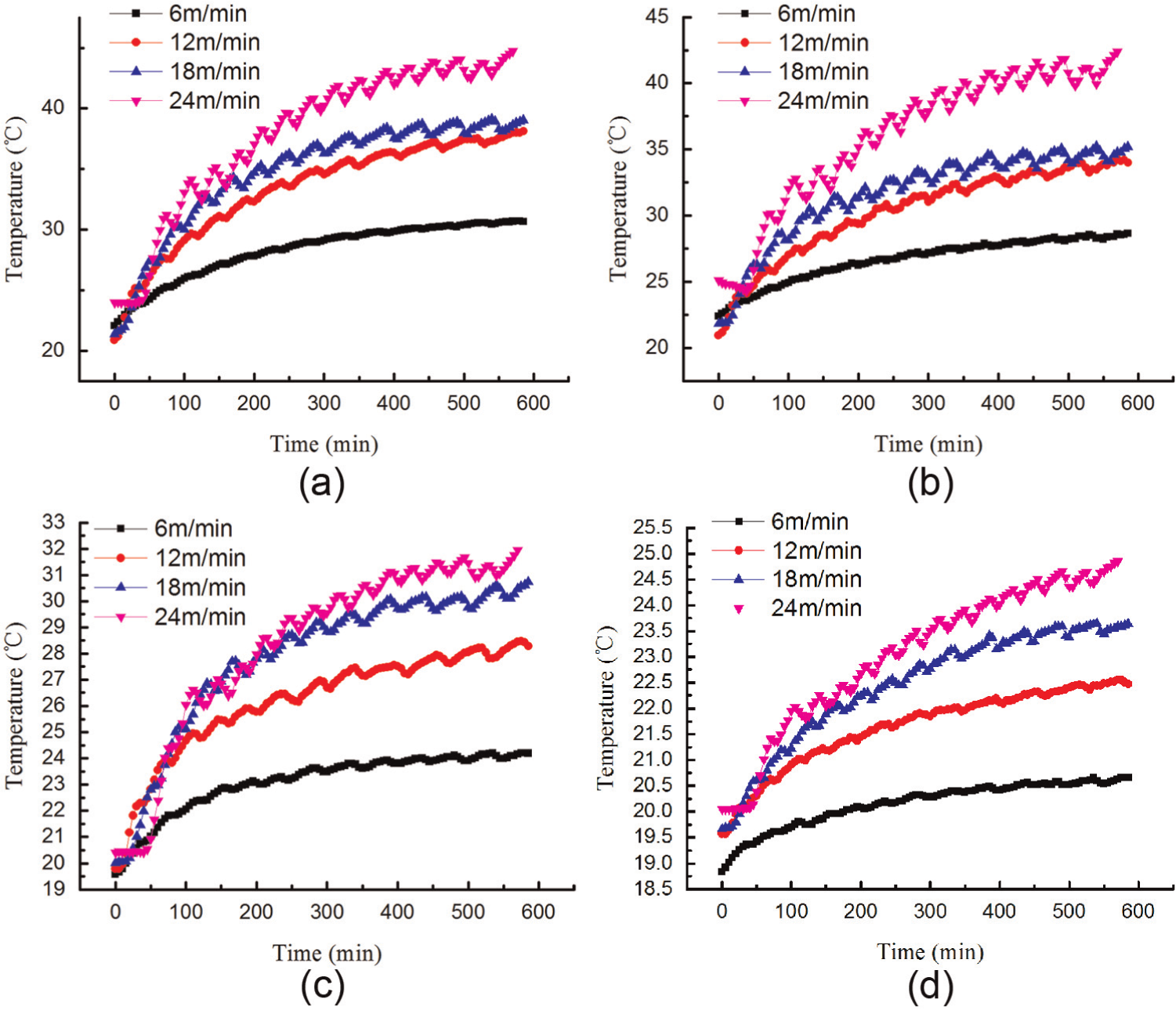
Measured temperatures: (a) upper motor, (b) lower motor, (c) upper bearing, and (d) lower bearing.

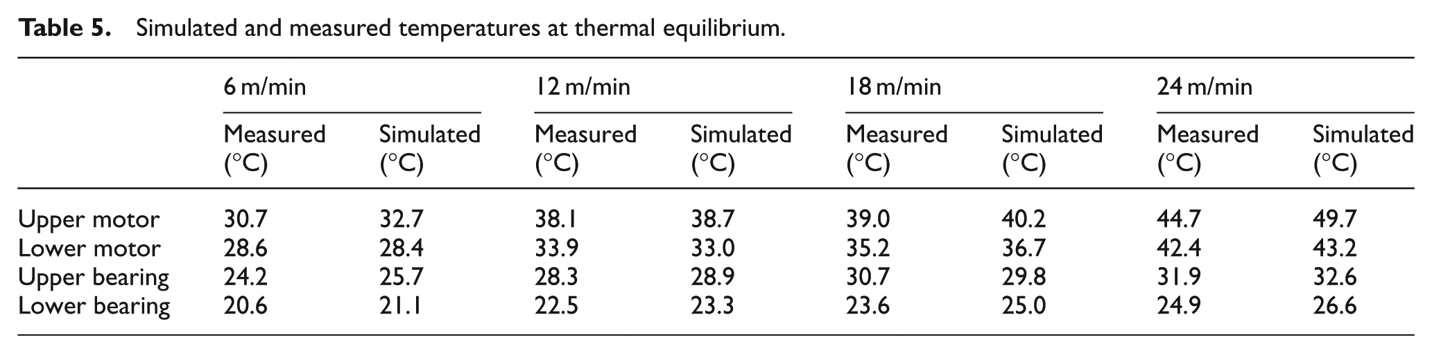
The measured part temperatures were compared with the simulated values, as shown in Table 5, of the thermal equilibrium at four feed rates. The temperatures increased with increases in the feed rate. For F = 24 m/min, the measured temperature of the upper active control motor reached 44.7 °C, in good agreement with the simulated value of 49.7 °C; the maximum error of the simulation is 5 °C. The upper motor temperature was higher than the lower driven motor, which reached 42.4 °C. The measured upper bearing temperature was 31.9 °C, consistent with the simulated value of 32.6 °C, and it was clearly higher than the lower bearing temperature of 24.9 °C, similar to the simulated value of 26.6 °C. Therefore, the experiments further verified the uneven temperature distribution of the dual-drive servo system between the upper and lower parts of the structure, which results in the thermal deformation.

Table 5.

Simulated and measured temperatures at thermal equilibrium.

	6 m/min		12 m/min		18 m/min		24 m/min
	Measured (°C)	Simulated (°C)	Measured (°C)	Simulated (°C)	Measured (°C)	Simulated (°C)	Measured (°C)	Simulated (°C)
Upper motor	30.7	32.7	38.1	38.7	39.0	40.2	44.7	49.7
Lower motor	28.6	28.4	33.9	33.0	35.2	36.7	42.4	43.2
Upper bearing	24.2	25.7	28.3	28.9	30.7	29.8	31.9	32.6
Lower bearing	20.6	21.1	22.5	23.3	23.6	25.0	24.9	26.6

Figures 11 and 12 show comparisons between the simulated and the measured temperatures of 12 measurement points on the screw at a feed rate of 24 m/min. In the experiments, the temperatures of the measured points at 50 and 150 mm are slightly higher than the others, as these two points near the motor and thus receive more heat. With the exception of these two points, the results indicate that the temperatures of the others are similar, and they fluctuate within 1.5 °C. Therefore, the entire screw temperature field approximates an isothermal surface, as shown in Figures 11(b) and 12(b). The highest temperature in the simulation is 25.5 °C, which is lower than the measured value of 27.8 °C.

Figure 11.

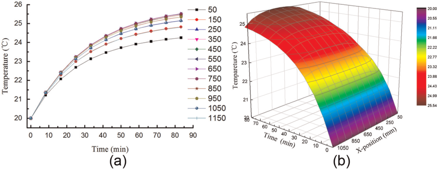
Simulated temperatures of the screw at F = 24 m/min: (a) with time and (b) with time and position.

Figure 12.

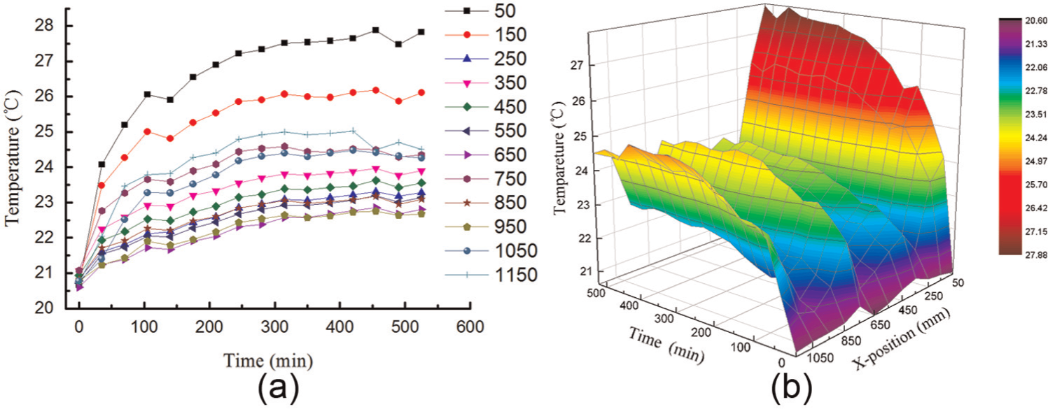
Measured temperatures of the screw at F = 24 m/min: (a) with time and (b) with time and position.

In addition, the temperatures in the middle region of the stroke on the screw are higher than other points, mainly due to the friction caused by the movement of the slider within this range, which generated substantial heat. Additionally, the machine space is relatively closed, making heat dissipation more difficult and therefore generating higher temperatures at the points in the measuring range.

We took the average temperature of all the measured points at each time to characterise the typical screw temperature. The measured and simulated values are shown in Figures 13 and 14 for different feed rates. The average temperature at the thermal steady state increased with higher feed rates. As shown in Figure 13(b), the temperature and feed rate have an approximately exponential relationship.

Figure 13.

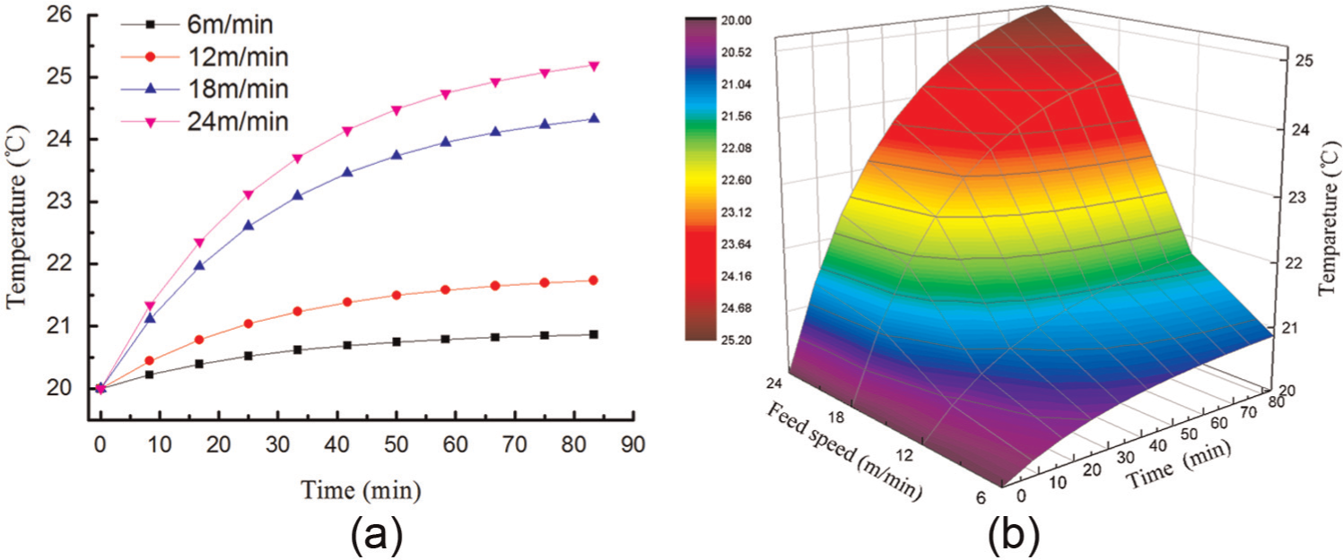
Average value of the simulated screw temperature: (a) with time and (b) with time and feed rate.

Figure 14.

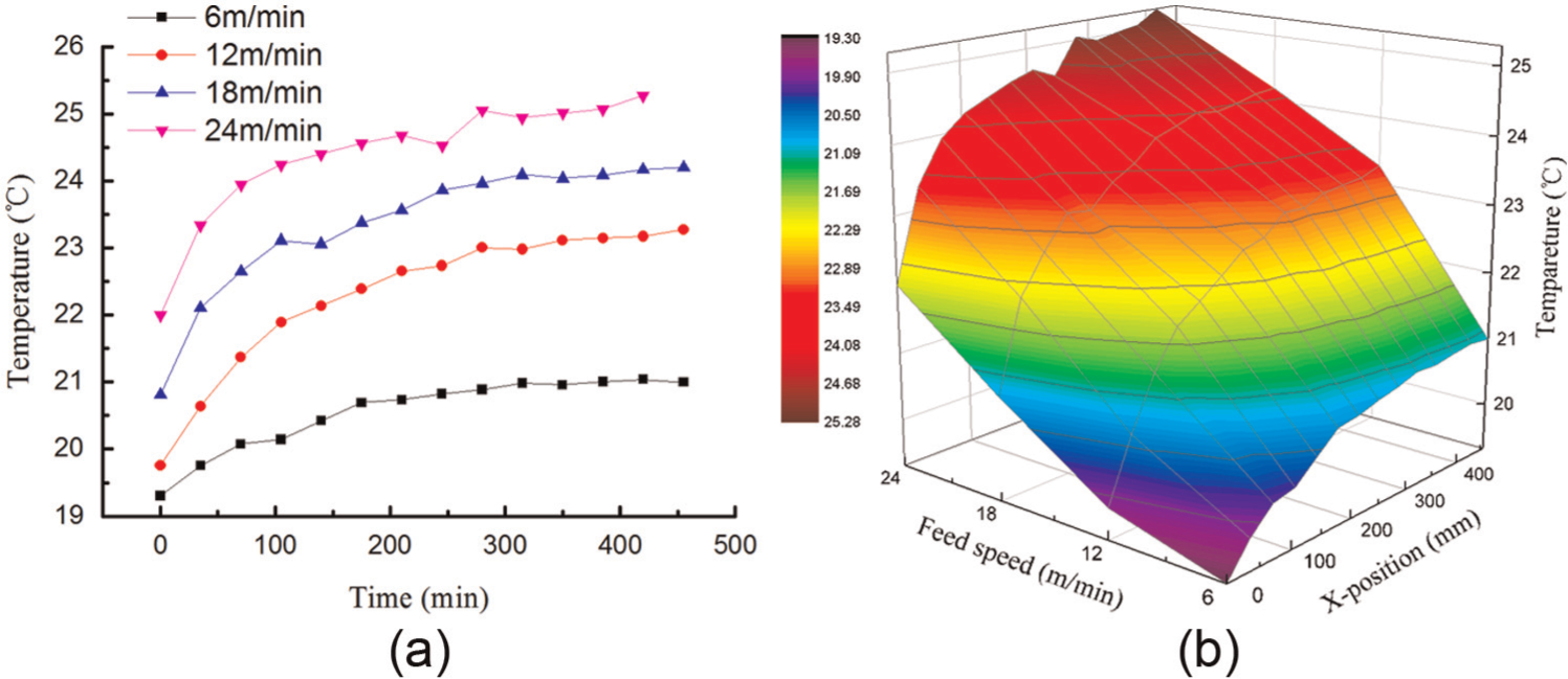
Average value of the measured screw temperature: (a) with time and (b) with time and feed rate.

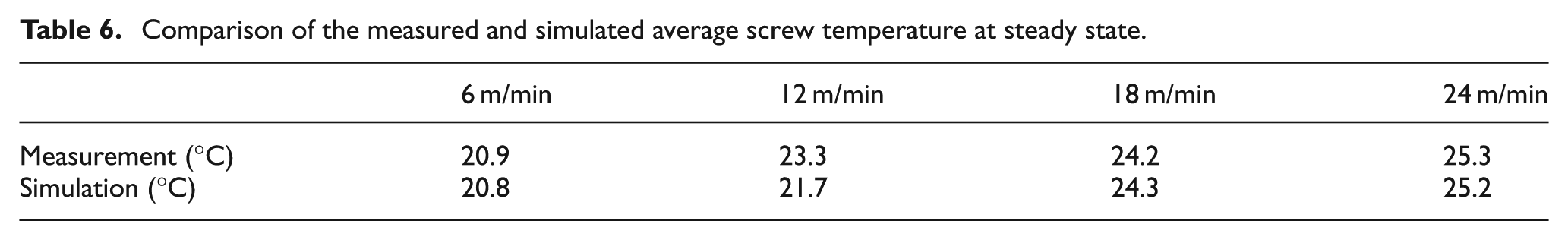
The average measured and simulated temperatures of the screw at the thermal steady state are presented in Table 6. The errors between the simulation and the measurement are within 1.6 °C, showing the effectiveness of the FEM model.

Table 6.

Comparison of the measured and simulated average screw temperature at steady state.

	6 m/min	12 m/min	18 m/min	24 m/min
Measurement (°C)	20.9	23.3	24.2	25.3
Simulation (°C)	20.8	21.7	24.3	25.2

Comparison of the simulated and measured thermal error

Although many complex factors can cause thermal errors of the feed axis, the position and feed rate are the most important. First, the time-domain characteristics, position distribution, and spatial field of the thermal error in the X-axis were analysed at a feed rate of 24 m/min. Second, three measurement points were chosen to analyse the influence of feed rates on the corresponding thermal errors. Finally, the thermal error distribution statuses at the thermal steady state were compared at different feed rates.

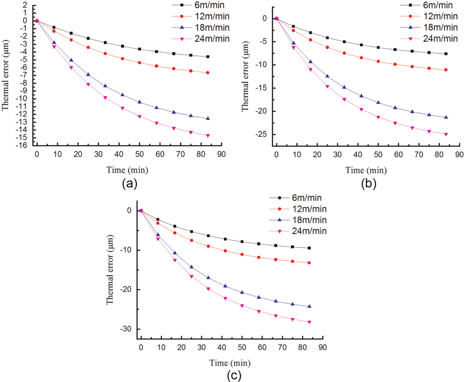
The simulated and experimental results at 24 m/min are shown in Figures 15 and 16. The maximum thermal errors in both the simulation and the experiment occurred at 1150 mm; the former was 27.5 μm and the latter was 26.7 μm at thermal equilibrium. Figures 15(a) and 16(a) show the variation of thermal errors over time, and the thermal error and time exhibited an approximately exponential relationship. Figures 15(b) and 16(b) indicate that the relationship of the thermal error of the feed axis with position is approximately linear. Figures 15(c) and 16(c) directly reflect the relationship of the thermal error with time and position.

Figure 15.

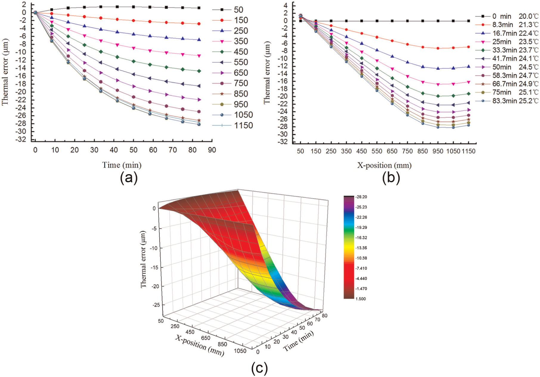
Simulated thermal errors at F = 24 m/min: (a) with time, (b) with position, and (c) with position and time.

Figure 16.

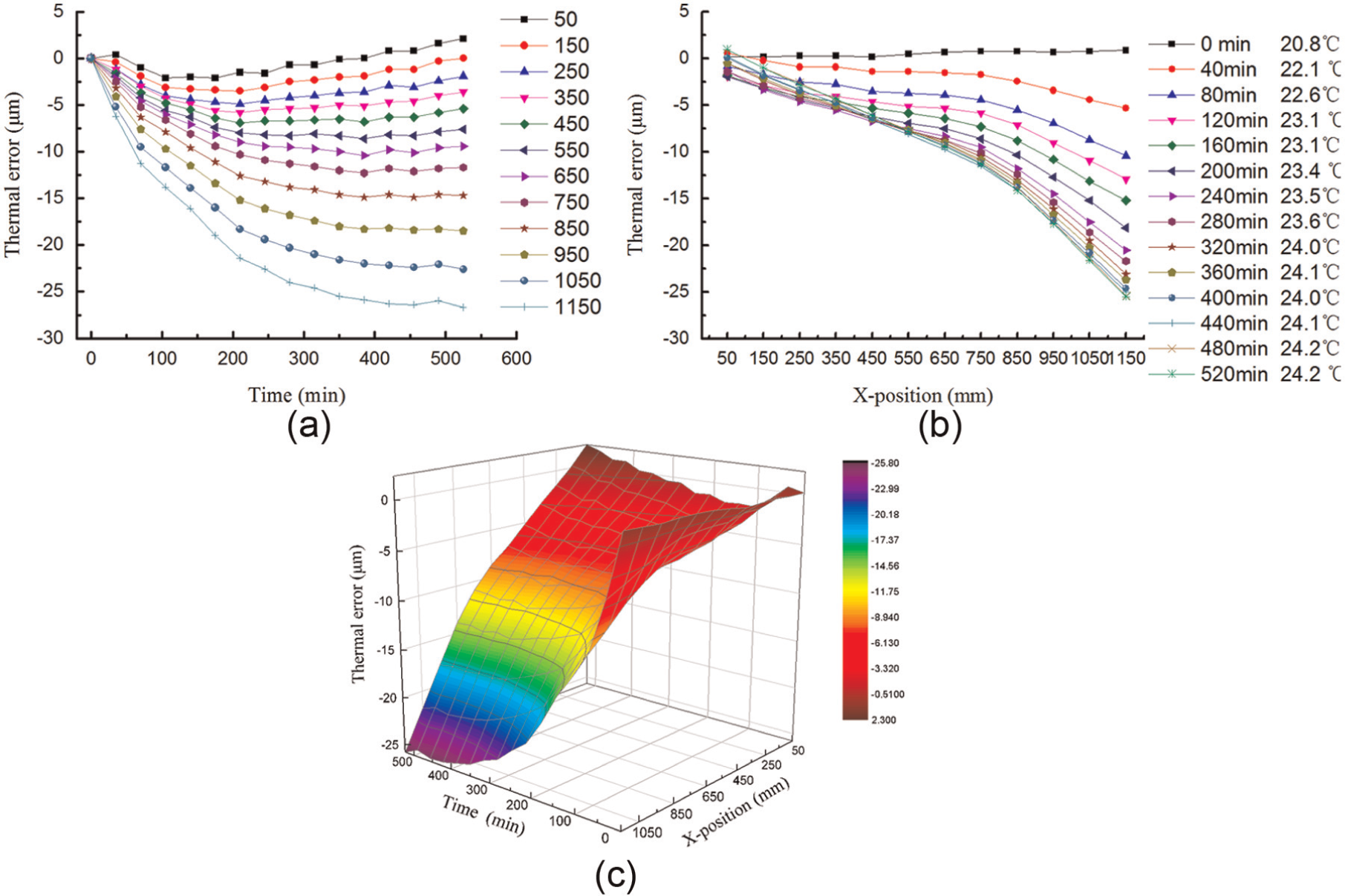
Measured thermal errors at F = 24 m/min: (a) with time, (b) with position, and (c) with position and time.

To study the influences of feed rate on the thermal error at different positions, three measurement points on the X-axis were chosen as follows: 450, 750, and 1050 mm. Figure 17 shows that at a particular feed rate, the thermal error increases along with position. Meanwhile, the thermal error increases with increased feed rates for a particular point. The measurement results are shown in Figure 18 and match well with the simulation. As shown in Table 5, the deviation between the simulation and the measurement is within 8.3 μm at 450 mm, and the deviation is approximately 5.7 μm at 1050 mm at the steady state at F = 24 m/min.

Figure 17.

Simulated thermal error in the X-axis: (a) 450-mm position, (b) 750-mm position, and (c) 1050-mm position.

Figure 18.

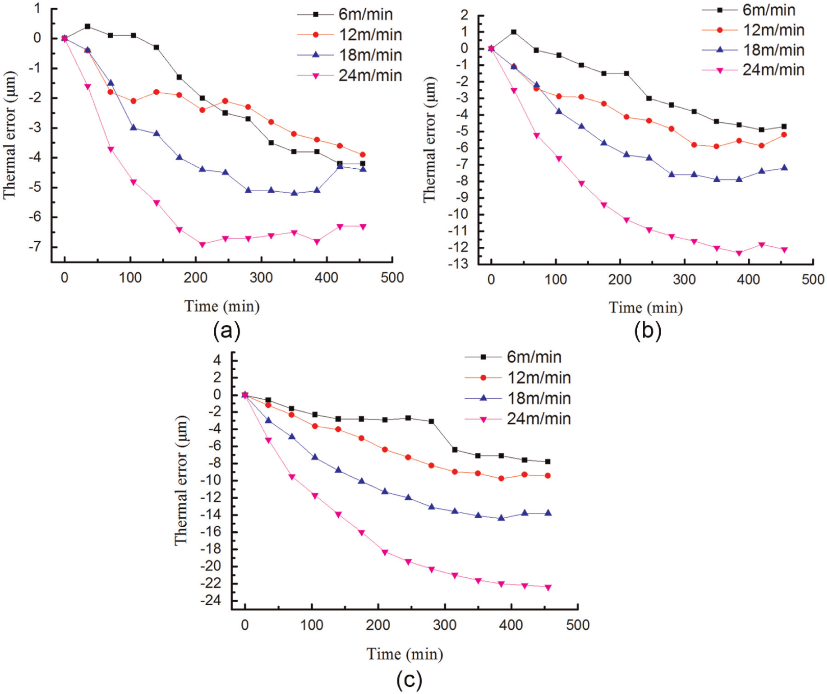
Measured thermal error in the X-axis: (a) 450-mm position, (b) 750-mm position, and (c) 1050-mm position.

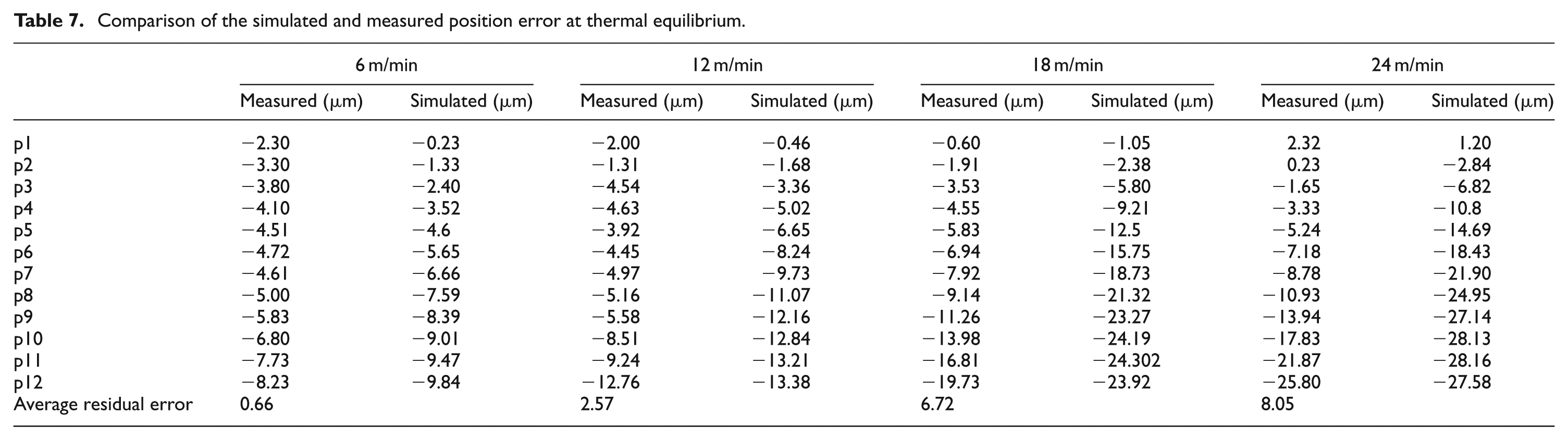
In the thermal equilibrium state, the thermal error distribution along the X-axis at different feed rates is shown in Figures 19 and 20 and Table 7. At feed rates of 6, 12, 18, and 24 m/min, the corresponding average residual errors between the simulation and the measurement were 0.66, 2.57, 6.72, and 8.05 μm, respectively. This result clearly shows that the thermal errors calculated by FEM fit the measured values well, effectively demonstrating the accuracy of the finite element model and the boundary conditions.

Figure 19.

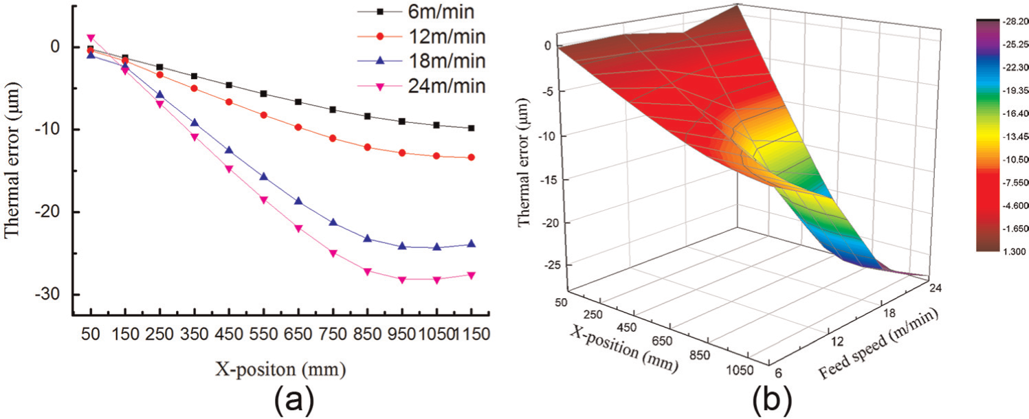
Simulated thermal error at thermal equilibrium: (a) with position and (b) with position and feed rate.

Figure 20.

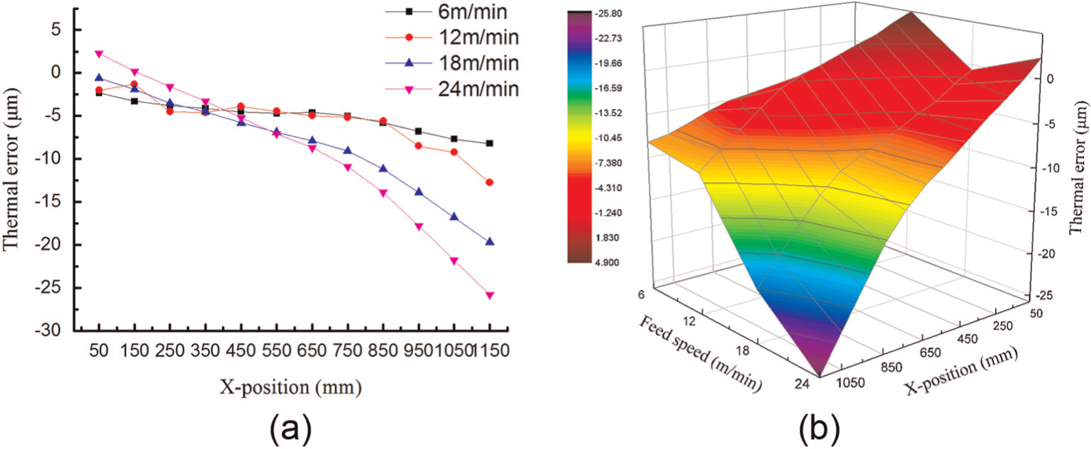
Measured thermal error at thermal equilibrium: (a) with position and (b) with position and feed rate.

Table 7.

Comparison of the simulated and measured position error at thermal equilibrium.

	6 m/min		12 m/min		18 m/min		24 m/min
	Measured (μm)	Simulated (μm)	Measured (μm)	Simulated (μm)	Measured (μm)	Simulated (μm)	Measured (μm)	Simulated (μm)
p1	−2.30	−0.23	−2.00	−0.46	−0.60	−1.05	2.32	1.20
p2	−3.30	−1.33	−1.31	−1.68	−1.91	−2.38	0.23	−2.84
p3	−3.80	−2.40	−4.54	−3.36	−3.53	−5.80	−1.65	−6.82
p4	−4.10	−3.52	−4.63	−5.02	−4.55	−9.21	−3.33	−10.8
p5	−4.51	−4.6	−3.92	−6.65	−5.83	−12.5	−5.24	−14.69
p6	−4.72	−5.65	−4.45	−8.24	−6.94	−15.75	−7.18	−18.43
p7	−4.61	−6.66	−4.97	−9.73	−7.92	−18.73	−8.78	−21.90
p8	−5.00	−7.59	−5.16	−11.07	−9.14	−21.32	−10.93	−24.95
p9	−5.83	−8.39	−5.58	−12.16	−11.26	−23.27	−13.94	−27.14
p10	−6.80	−9.01	−8.51	−12.84	−13.98	−24.19	−17.83	−28.13
p11	−7.73	−9.47	−9.24	−13.21	−16.81	−24.302	−21.87	−28.16
p12	−8.23	−9.84	−12.76	−13.38	−19.73	−23.92	−25.80	−27.58
Average residual error	0.66		2.57		6.72		8.05

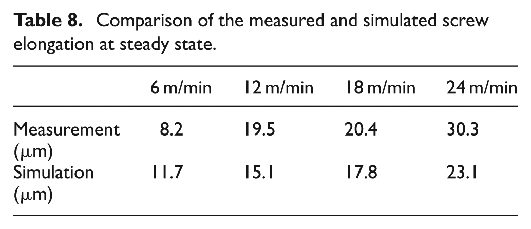
The comparison of the screw terminal elongation between the simulation and the measurement at thermal equilibrium is described in Table 8. The maximum error was 7.2 μm at 24 m/min, and the error between the experiment and the simulation was approximately 4 μm at other feed rates. This result indicates that the thermal deformation calculated by FEM is close to the measured data.

Table 8.

Comparison of the measured and simulated screw elongation at steady state.

	6 m/min	12 m/min	18 m/min	24 m/min
Measurement (μm)	8.2	19.5	20.4	30.3
Simulation (μm)	11.7	15.1	17.8	23.1

Thermal error modelling and compensation for the feed axis

Thermal errors in the feed system are related to coordinate position, temperature, and other parameters.^35,36 Here, the mapping relationships of the thermal error with thermal equilibrium time, coordinate position, and typical characteristic temperature were established by analysing the experimental data and then constructing an integrated mathematical model of thermal error. Next, the integrated model was used to predict the thermal error with a new data sample, and the predicted values were compared with the experimental measurements to verify the accuracy and versatility of the model. Finally, thermal error compensation was performed on the X-axis. The following performance was based on an 18 m/min feed rate, and the thermal error distribution is shown in Figure 21.

Figure 21.

Measured thermal error on the X-axis at F = 18 m/min.

Thermal error modelling

Thermal error time function

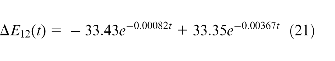
Figure 22 presents the curve fitting for the thermal error at −1150 mm at time t. From the analysis, the thermal error is a second-order exponential function with time

Δ E_{12} (t) = - 33.43 e^{- 0.00082 t} + 33.35 e^{- 0.00367 t}

(21)

Figure 22.

Thermal deformation curve fit over time.

ΔE ₁₂(t) is the thermal error at time t for the 12th measurement point (at −1150 mm). The coefficient of determination, R-squared, or R_s , can then be calculated with a boundary region of [0, 1], thereby characterising the extent to which the original data fall along the curve at a certain confidence level. A larger R_s value indicates that the curve fits the original data better, meaning that the argument for explaining the model is more powerful. The root squared mean error (RSME) of the fitted and measured values is denoted by R_m , which indicates how closely the curve fits the original measurement data; a smaller value (closer to 0) indicates that the original data are more concentrated on both sides around the fitted curve. The calculations indicated that R_s = 0.9990 and R_m = 0.1985; these two evaluation methods show that the non-linear relationship of the axial thermal error over time is significant.

Thermal error function of the position coordinates

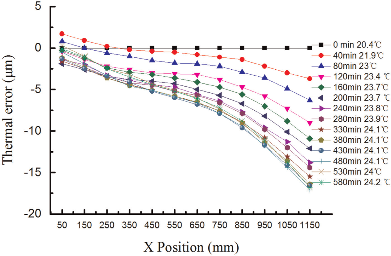
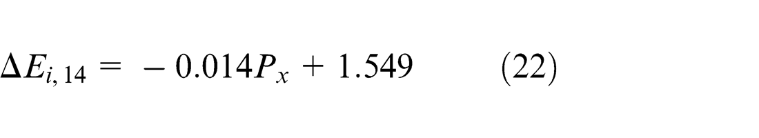
The final measurement data from the precision machine tools were used as the sample space of the model. The screw characteristic temperature, T ₁₄ = 24.2 °C, was calculated using equation (20), and the distribution of the thermal error for the measurement points is shown in Figure 23. The fitting function was obtained using the following linear approximation

Δ E_{i, 14} = - 0.014 P_{x} + 1.549

(22)

Figure 23.

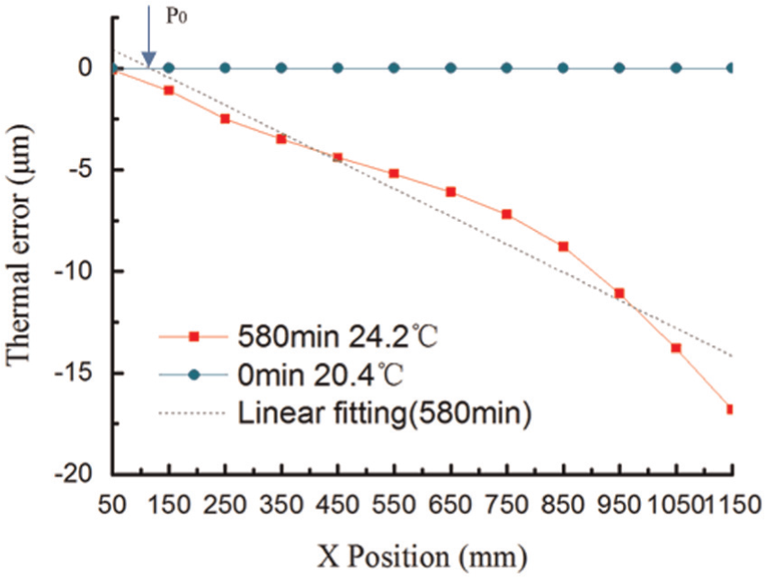
Thermal error of the X-axis at 580 min.

where ΔE_i_,14 is the ith measurement point of the 14th measured thermal error and P_x represents the coordinates of the ith measurement point. It was determined that R_s = 0.9452 and the residual RMSE R_m = 1.2548, indicating that the model perfectly fits the data and that there is a significant linear relationship between the screw thermal error and the coordinate position.

Assuming that a point on the screw exists where the thermal error is 0, this point is the reference point P ₀, where ΔE_i _,14 = 0. P ₀ was calculated using equation (22)

P_{0} = 112.409 mm

(23)

Thermal error function of temperature

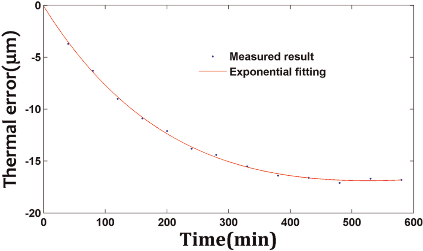
The screw terminal thermal elongation is the accumulation of the expansion of the entire screw. The screw is simplified as a linear rod, and the maximum thermal deformation of a linear rod is dependent on temperature. Figure 24 presents the exponential curve fit of the screw thermal deformation versus temperature, and the analytical expression is as follows

Δ E_{12, j} = - 3.049 \times 10^{- 8} e^{0.835 T_{j}}

(24)

Figure 24.

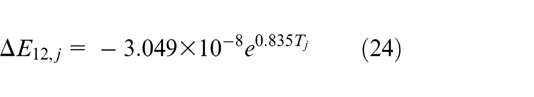
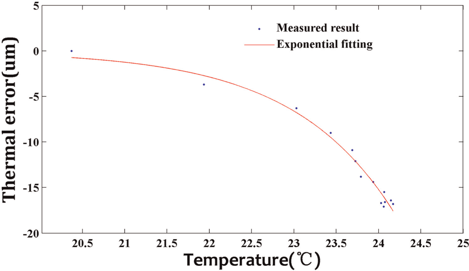
Comparison of the fitted values and measured thermal errors.

where ΔE _12,j is the thermal error of the measurement point at −1,150 mm, T_j is the screw typical characteristic temperature, the determination coefficient is R_s = 0.9799 and R_m = 0.8059, that is, the mapping function has a physical interpretation significance.

Thermal error integrated model

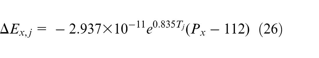
Equation (22) indicates that there is a linear relationship between the screw coordinate position and thermal error. Thus, assuming that the thermal deformation of a unit length of a screw is constant at a particular temperature, the following a ratio equation can be deduced

\frac{Δ E_{x, j}}{P_{x} - P_{0}} = \frac{Δ E_{12, j}}{1150 - P_{0}}

(25)

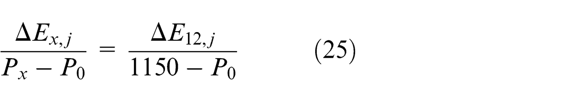
where P_x (mm) is the coordinate position, T_j (°C) is the characteristic temperature of the screw, and ΔE_x _,j (μm) is the thermal error of P_x when the temperature is T_j . As shown in equation (26), the thermal error ΔE_x _,j can be obtained by applying equations (23) to (25)

Δ E_{x, j} = - 2.937 \times 10^{- 11} e^{0.835 T_{j}} (P_{x} - 112)

(26)

Model validation

Figure 25 compares the model predictions with the measured values using equation (26) to predict the thermal error ΔE_x _,j of the measurement points on the feed axis at 480 min.

Figure 25.

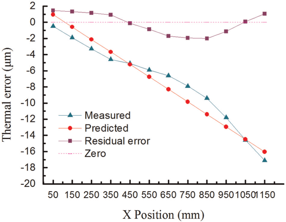
Comparison between the model predictions and experimentally measured results.

Under these conditions, the screw characteristic temperature is T_j = 24.1 °C. It was determined that the residual R_m = 1.283. Furthermore, the absolute mean of the residuals was 1.15 μm, and the absolute mean of the original thermal errors of the measurement point was 7.375 μm; thus, the predictive accuracy of the model is approximately 85%, indicating that the mathematical model can predict with high precision. The verification data represent a new sample space and can also achieve accurate prediction, indicating that the thermal error model also has high versatility.

Thermal error compensation

Using the feedback integration method, the compensation signal is superimposed on the original coordinate value, forming a new coordinate in the position loop on the CNC system; the new position coordinate is used to control the movement of the motor so as to ultimately achieve thermal error compensation. Figure 26 is a schematic diagram of the thermal error compensation used with the Siemens 840D CNC system. The thermal drift module acquires signals from the PT100 units and sends them to the PC via USB. The computer then establishes a thermal model and calculates the error offset. Next, the error offset is sent to the Programmable Logic Controller (PLC) through the Human Machine Interface (HMI) on the CNC system. The thermal error compensation module is embedded into the CNC based on the secondary development of the 840D, and it can receive error compensation parameters and pass them to the PLC. Finally, the thermal error offset is inserted into the position loop, and compensation is achieved.

Figure 26.

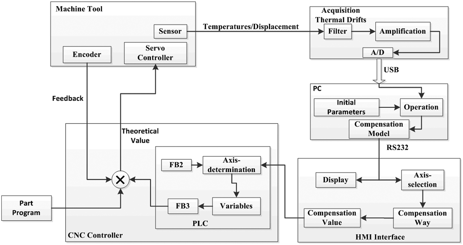
Thermal error compensation control.

The real-time thermal offset was calculated by applying equation (26), and the error compensation result is presented in Figure 27. At a feed rate of 18 m/min, the maximum error decreased from −6.3 to −1.0 μm in the X direction at 22.6 °C, and accuracy was improved by 73%. At 24.1 °C, the maximum error was reduced from −16.7 to −4.5 μm, and accuracy was increased by 62%. These results demonstrate the effectiveness of the proposed measurement method and the modelling.

Figure 27.

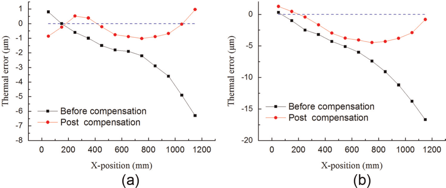
Thermal error compensation along the X-axis at 18 m/min: (a) at 22.6 °C and (b) at 24.1 °C.

Conclusion

In this article, a systematic method is presented to analyse the thermal behaviour of a jig-boring machine equipped with a dual-drive servo feed system. The method includes transient simulation, measurement, modelling and compensation. A set of systematic solutions is proposed to study thermal error compensation technology and to effectively improve machining accuracy for industrial applications. From the results, the following conclusions can be drawn:

A thermal–structure FEM model for the machine was developed, and the boundary conditions, such as the heat generation principle of the motors, bearings, and screw, as well as the convection heat transfer coefficient, were considered. The transient temperature distribution and thermal deformation of the feed system were analysed at different feed rates. Comparison between the measured and the simulated results showed very good agreement.

The three linear axes of the machine are synchronised in a dual-drive configuration. However, the load and preload forces of each screw are not even, and the control of the dual-drive servo motors cannot be precisely synchronised, both of which can easily lead to uneven temperature gradient distributions. Such uneven distributions can result in linear expansion or bending and twisting of the screw in the 3D space, eventually resulting in thermal errors that decrease machining accuracy.

A synchronous acquisition system was developed to measure temperatures and thermal deformations. The temperatures of moving parts, such as the screw and worktable, were obtained by the infrared thermography, while the temperatures of the motors, the bearings, the base and the environment were collected by magnetic PT100 units. Together, these sensors achieved a dynamic measurement of the temperature field during running. In addition, the thermal deformations are measured by two components. The position-dependent thermal errors in the feed axis are measured by a laser interferometer, while the screw terminal thermal expansion is acquired by an eddy-current sensor, enabling integrated monitoring of the thermal deformation in the feed axis.

The mapping relationships of the thermal error with thermal equilibrium time, coordinate position, and typical characteristic temperature were established by analysing the experimental data. An integrated mathematical thermal error model with an accurate predictive capacity was then constructed. Finally, thermal error compensation was implemented by applying a feedback integration method. The thermal errors were compensated under two conditions, 24.1 °C and 22.6 °C, at a feed rate of 18 m/min. The results showed that the machining precision was increased by 73% and 62% at 24.1 °C and 22.6 °C, respectively.

Footnotes

Declaration of conflicting interests

The authors declare that they have no financial and personal relationships with other people or organisations that can inappropriately influence our work; there is no professional or other personal interest of any nature or kind in any product or company that could be construed as influencing the position presented in, or the review of, the article.

Funding

This research was supported by the National High-Tech R&D Program of China (863 Program) under Grant Number 2012AA040701.

References

Bryan

. International status of thermal error research. CIRP Ann: Manuf Techn 1990; 39(2): 645–656.

Mou

. A method of using neural networks and inverse kinematics for machine tool error estimation and correction. J Manuf Sci E: T ASME 1997; 119: 247–254.

Zhang

Mei

Shao

. An improved holospectrum-based balancing method for rotor systems with anisotropic stiffness. Proc IMechE, Part C: J Mechanical Engineering Science 2013; 227(2): 246–260.

Kung

. Thermal analysis for the feed drive system of a CNC machine center. Int J Mach Tool Manu 2003; l43: 1521–1528.

Mian

Fletcher

Longstaff

. Efficient thermal error prediction in a machine tool using finite element analysis. Meas Sci Technol 2011; 22(8): 365–372.

Min

Jiang

. A thermal model of a ball screw drive system for a machine tool. Proc IMechE, Part C: J Mechanical Engineering Science 2011; 225(1): 186–225.

Won

Soo

Dong

. Thermal error analysis for a CNC lathe feed drive system. Int J Mach Tool Manu 1999; 39(7): 1087–1101.

Kima

Jeong

Cho

. Thermal behavior of a machine tool equipped with linear motors. Int J Mach Tool Manu 2004; 44: 749–758.

Uhlmann

. Thermal modeling of an HSC machining centre to predict thermal error of the feed system. Prod Engineer (WGP) 2012; 6: 603–610.

10.

Chen

Chiou

. Quick testing and modeling of thermally-induced errors of CNC machine tools. Int J Mach Tool Manu 1995; 35(7): 1063–1074.

11.

Yang

Yuan

. The improvement of thermal error modeling and compensation on machine tools by CMAC neural network. Int J Mach Tool Manu 1996; 36(4): 527–537.

12.

Chen

. Fast calibration and modeling of thermally-induced machine tool errors in real machining. Int J Mach Tool Manu 1997; 37(2): 159–169.

13.

Wang

Tseng

Kuoming

LIN

. Thermal error modeling of a machining center using grey system theory and adaptive network-based fuzzy inference system. JSME Int J C: Mech Sy 2007; 49(4): 1179–1187.

14.

Mize

Ziegert

. Neural network thermal error compensation of a machining center. Precis Eng 2000; 24(4): 338–346.

15.

Ramesh

Mannan

Poo

. Support vector machines model for classification of thermal error in machine tools. Int J Adv Manuf Tech 2002; 20(2): 114–120.

16.

Postlethwaite

Allen

Ford

. Use of thermal imaging, temperature and distortion models for machine tool thermal error reduction. Proc IMechE, Part B: J Engineering Manufacture 1998; 212(8): 671–679.

17.

Wang

Huang

Yang

. In-line statistical monitoring of machine tool thermal error through latent variable modeling. J Manuf Syst 2006; 25(4): 279–292.

18.

Pahk

Lee

. Thermal error measurement and real time compensation system for the CNC machine tools incorporating the spindle thermal error and the feed axis thermal error. Int J Adv Manuf Tech 2002; 20(7): 487–494.

19.

Postlethwaite

Allen

Ford

. Machine tool thermal error reduction – an appraisal. Proc IMechE, Part B: J Engineering Manufacture 1999; 213(1): 1–9.

20.

Yang

. Dynamic modeling for machine tool thermal error compensation. J Manuf Sci E: T ASME 2003; 125(2): 245–254.

21.

Yang

Yao

. Modeling approach of regression orthogonal experiment design for the thermal error compensation of a CNC turning center. J Mater Process Tech 2002; 129(1–3): 619–623.

22.

Zhao

. Axial thermal error compensation method for the spindle of a precision horizontal machining center. In: 2012 IEEE international conference on mechatronics and automation, ICMA, Chengdu, China, 5–8 August 2012, pp.2319–2323. New York: IEEE.

23.

Gebhardt

Mayr

Furrer

. High precision grey-box model for compensation of thermal errors on five-axis machines. CIRP Ann: Manuf Techn 2014; 63: 509–512.

24.

Pajor

Zapata

. Supervising and compensation of thermal error of CNC feed ball screw. Diagnostyka 2013; 14(2): 37–42.

25.

Miao

Gong

Niu

. Robustness of thermal error compensation modeling models of CNC machine tools. Int J Adv Manuf Tech 2013; 69(9–12): 2593–2603.

26.

Wang

Yang

. A combined error model for thermal error compensation of machine tools. Adv Mat Res 2013; 820: 147–150.

27.

Zhang

Yang

Xiang

. Volumetric error modeling and compensation considering thermal effect on five-axis machine tools. Proc IMechE, Part C: J Mechanical Engineering Science 2013; 227(5): 1102–1115.

28.

Baehr

Stephan

. Wärme- und Stoffübertragung. Berlin: Springer, 2009.

29.

Frank

Incropera

. Fundamentals of heat and mass transfer. London: SOS Free Stock, 2001.

30.

Harris

. Rolling bearing analysis. New York: John Wiley & Sons, 1991, pp.540–560.

31.

Harris

. Rolling bearing application. Beijing, China: China Machine Press, 2014.

32.

Zhao

Yang

Shen

. Simulation of thermal behavior of a CNC machine tool spindle. Int J Mach Tool Manu 2007; 47(6): 1003–1010.

33.

Palmgern

. Ball and roller bearings. Philadelphia, PA: S.H. Burbank, 1959.

34.

Eugene

Theodore

. Marks’ standard handbook for mechanical engineers. 10th ed. New York: McGraw-Hill Professional, 2007.

35.

Srivastava

Veldhuis

Elbestawit

. Modeling geometric and thermal errors in a five-axis CNC machine tool. Int J Mach Tool Manu 1995; 35(9): 1321–1337.

36.

Siemens. SINUMERIK 840D sl/840Di sl/840D/840Di/810D extended functions, 2006, pp.353–356, http://www.automation.siemens.com/doconweb/pdf/SINUMERIK_SIMODRIVE_04_2010_E/FB2.pdf?p=1

Thermal error simulation and compensation in a jig-boring machine equipped with a dual-drive servo feed system

Abstract

Keywords

Introduction

Thermal behaviour simulation

FEM

Heat transfer coefficient

Power calculation of the heat sources

Computation of the screw thermal generation

Bearing thermal generation model

Motor heat generation model

Transient simulation analysis

Temperature field characteristics

Thermal deformation of the feed system

Experimental verification

Experimental system

Measurement principle

Results and analysis

Comparison of the simulated and the measured temperature

Comparison of the simulated and measured thermal error

Thermal error modelling and compensation for the feed axis

Thermal error modelling

Thermal error time function

Thermal error function of the position coordinates

Thermal error function of temperature

Thermal error integrated model

Model validation

Thermal error compensation

Conclusion

Footnotes

Declaration of conflicting interests

Funding

References