Applying mechanical equilibrium rules in project cost management

Abstract

The earned value management is a systematic approach to measure project progress and forecast final cost of a project. However, this method has not significantly been improved over its earlier version and there are some criticisms against this standard method. This approach presents a good condition if only the cost performance index shows satisfactory results. The objective of this research is to propose a new methodology in project financial system according to the rules and regulations on mechanical equilibrium of a beam. The results have been successfully implemented which improved the standard project cost management system.

Introduction

The earned value management (EVM) is a well-known project management system which integrates cost, schedule and scope of work. It helps to calculate performance indices and predicts project total duration and cost. The EVM prepares early indicators of project performance to emphasize needs for potential corrective actions. Originally, the EVM was initially developed for project cost analysis; however, now it has become one of the important branches of a project management system.

EVM measures

The standard EVM has three important measures: earned value (EV) or budgeted cost of the work completed, planned value (PV) or budget cost of the work scheduled and actual cost (AC) or expenditures of the work performed. Also, there are some additional components in the EVM literature which are summarized as follows:

• Scheduled variance (SV = EV − PV)

• Cost variance (CV = EV − AC)

• Scheduled performance index (SPI = EV/PV)

• Cost performance index (CPI = EV/AC)

Deviations in different cases are expressed as follows:

• CPI or CV

• CPI = 1 or CV = 0: on budget situation.

• CPI > 1 or CV > 0: the cost of the project is less than planned.

• CPI < 1 or CV < 0: the cost of the project is more than planned.

• SPI or SV

• SPI = 1 or SV = 0: on schedule situation.

• SPI > 1 or SV > 0: duration of the project is less than planned.

• SPI < 1 or SV < 0: duration of the project is more than planned.

EV literature

Related studies in the EVM area mostly concentrated on its developments. Initially, to overcome some limitations of EV in forecasting of project performance, several models have been developed. Christensen ¹ proposed new indexes to evaluate the accuracy of the estimate at completion. Zwikael et al. ² evaluate five prediction methods. Christensen and Templin ³ justify the usability of two Estimate at Completion (EAC) evaluation methods by means of statistical evidence from a sample of defense acquisition contracts. Vandevoorde and Vanhoucke ⁴ compared three different approaches to predict project duration by EV metrics and appraise them on real-life project data. Lipke et al. ⁵ studied statistical confidence limits to improve estimates at completion. Kim and Reinschmidt ⁶ proposed a new probabilistic prediction method based on the beta distribution and Bayesian inference which integrates original estimates with observations of new actual performance. Moselhi ⁷ proposed a new concept for the SPI to measure the status of critical activities only, and this index is used to predict project duration. Bagherpour and Noori ⁸ proposed a new approach to apply EVM in multi-period–multi-product (MPMP) production planning problem. Bagherpour et al. ⁹ improved manufacturing profitability index with implementation of activity-based costing and time-driven activity-based costing techniques. Chang et al. ¹⁰ proposed a new method for capability performance analysis in production processes. They applied an accuracy index and a precision index to reflect the degree of deviation from target values and the degree of variance.

Although several researches had been carried out in the area of EVM, most of them concentrated on the applications of EVM in different cases. However, to the best of our knowledge, no related research was found in which provided equilibrium condition in project cost management systems which in this article mechanical equilibrium had been applied through project cost management systems.

Beams

A beam is an important element of a structure which is able to tolerate load, primarily by resisting bending. The bending force of the beam is a result of the own weight and external loads. When the beam is in equilibrium, it is not moving or rotating or the linear and angular accelerations are both 0. If the beam remains stationary (i.e. static) or its center of mass does not move, the resultant forces on the beam must be equal to 0. Similarly, if the beam does not rotate, the torque on the beam must be equal to 0. The concept of equilibrium is summarized as follows ¹¹

$$\sum F=0$$

(1)

$$\sum M=0$$

(2)

$$M=\mathrm{FX}$$

(3)

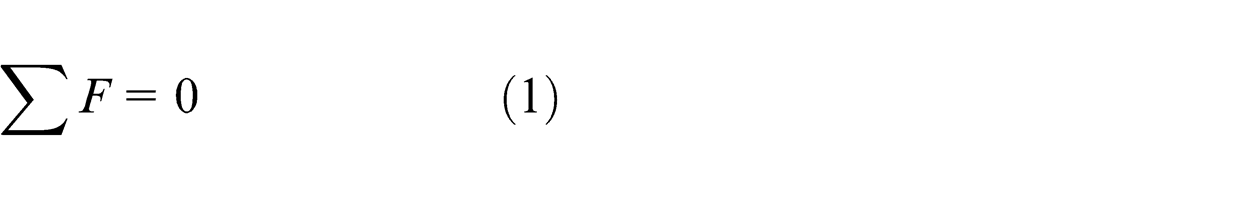
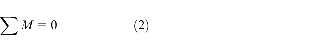
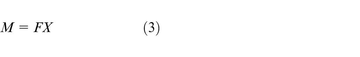
where F is the force, M is the torque and X is the distance.

1. When the resultant force on a beam is 0 (equation (1)), the beam is in force equilibrium. This means that its center of beam is either at rest or moving in a straight line with constant velocity.

2. When the resultant couple is 0 (equation (2)), the beam is in torque equilibrium, either having no rotational motion or rotating with a constant angular velocity.

3. When both resultants are 0, the body is in complete equilibrium.

To analyze the load-carrying capacities of a beam, we must first establish the equilibrium requirements of the beam as a whole and then any portion of it must be considered separately.

A shear force diagram will show how a load applied perpendicular to the axis of a beam is transmitted along the length of the beam. A bending moment diagram indicates how the applied loads to a beam create a moment variation along the length of the beam. The shear force and bending moment distributions can be calculated along the length of the beam by using the free-body diagram technique ¹¹ (e.g. Figure 1).

Figure 1.

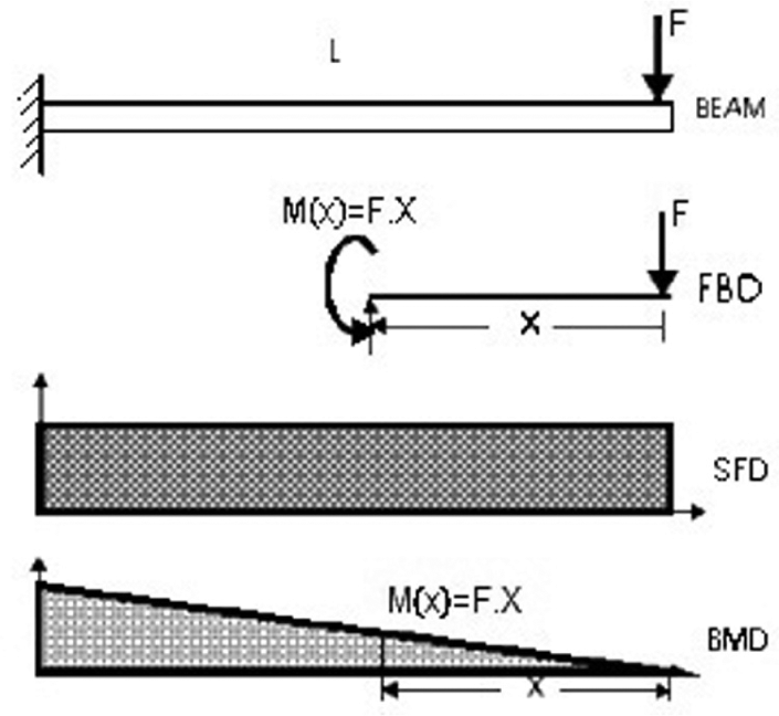
Free-body diagram of the beam, shear force and bending moment.

The variation in shear force (V) and bending moment (M) over the length of a beam provides necessary information for beam analysis. The variations in shear and moment will be displayed better in a graphical form. ¹¹

Determination of the values of all external loads on the beam is the first step to detect the moment and shear to establish the equations of equilibrium for beam using a free-body diagram. At the next step, a portion of the beam is isolated, either right or left of an arbitrary transverse section. Then, by free-body diagram, the equilibrium equations calculate this isolated portion of the beam. These equations will yield expressions for the shear force and bending momentum acting on the isolated section. The portion of the beam which involves the smaller number of forces, either right or left of the arbitrary portion, usually yields the simpler solution. ¹¹ Free-body diagram is given in Figure 1.

Eventually, it is important to note that the calculations for V and M on each isolated portion must be consistent with the positive convention illustrated equilibrium.

Using beams’ equilibrium rules in project cost management

The EVM is used as an important method for investigating and measuring project progress; however, this method has received some criticisms. As mentioned above, CPI is an important feature in cost performance analysis. At each cut-off date, the last CPI is determined regardless of what previously has happened. Thus, it is possible that the project had a critical situation such as long delay or high cost overrun happened in some previous periods, but at the last cut-off date CPI = 1 and it apparently shows a good situation; however, in real case, the project is not in good condition and this leads to neglecting some previous shortages and pitfalls. For example, the project in early months shows low progress with low EV, and in the last months, progress has extremely increased and the project is completed on budget. Therefore, CPI = 1 does not necessarily guarantee equilibrium of a financial system. When the project faces delay or it has been temporarily stopped, owner payments will get postponed and this may lead to failure of the project because of the inability of contractor in tolerating costs and negative cash flow. Sometimes, contractors may tolerate this negative cash flow depending on their financial power or using external sources such as loan, and the project may be completed on budget and on time; in this situation, with regard to the depreciating monetary value, the contractor gains less profit especially when inflation rate is expected to be high. In addition, critical conditions throughout project lifespan should not be neglected. Therefore, existing an index to measure instability quantity and afterward establishing stability is necessary while project is executing especially at all cut-off date.

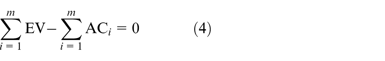
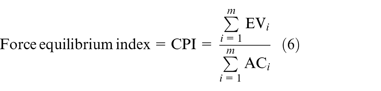
In this article, beam equilibrium rules are applied for solving this problem. Assume a project as a beam and AC and EV as loads that act on two sides of the beam against each other. To use beam equilibrium rules in project management area, all cut-off dates should be considered, and the resultant forces are calculated (AC and EV) in all cut-off dates. Afterward, stability indices should be calculated, and in case of project instability, the shortages must compensate in future periods to establish stable status. Similar to beam equilibrium rules, two indices are considered to investigate financial balance. The first index is derived from force equilibrium and it is another format of CPI in EVM which is explained in the following equation

$${\displaystyle \sum _{i=1}^m}\mathrm{EV}-{\displaystyle \sum _{i=1}^m}{\mathrm{AC}}_i=0$$

(4)

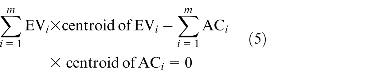
where i is the number of considered cut-off date for project, i = 1, 2, …, n, and m is the current cut-off date. The second index is derived by torque equilibrium. For torque equilibrium, a time interval is considered as distance, and this index is explained in the following equation

$$\begin{array}{c}\multicolumn{1}{c}{{\displaystyle \sum _{i=1}^m}{\mathrm{EV}}_i\times \mathrm{centroid}\mathrm{of}{\mathrm{EV}}_i-{\displaystyle \sum _{i=1}^m}{\mathrm{AC}}_i}\\ \multicolumn{1}{c}{\times \mathrm{centroid}\mathrm{of}{\mathrm{AC}}_i=0}\end{array}$$

(5)

These indices can be written as given below to create a comparable criterion of stability at different periods

$$\mathrm{Force}\mathrm{equilibrium}\mathrm{index}=\mathrm{CPI}=\frac{{\displaystyle \sum _{i=1}^m}{\mathrm{EV}}_i}{{\displaystyle \sum _{i=1}^m}{\mathrm{AC}}_i}$$

(6)

$$\mathrm{Torque}\mathrm{equilibrium}\mathrm{index}=\mathrm{TEI}=\frac{{\displaystyle \sum _{i=1}^m}{\mathrm{EV}}_i\times \mathrm{centroid}\mathrm{of}{\mathrm{EV}}_i}{{\displaystyle \sum _{i=1}^m}{\mathrm{AC}}_i\times \mathrm{centroid}\mathrm{of}{\mathrm{AC}}_i}$$

(7)

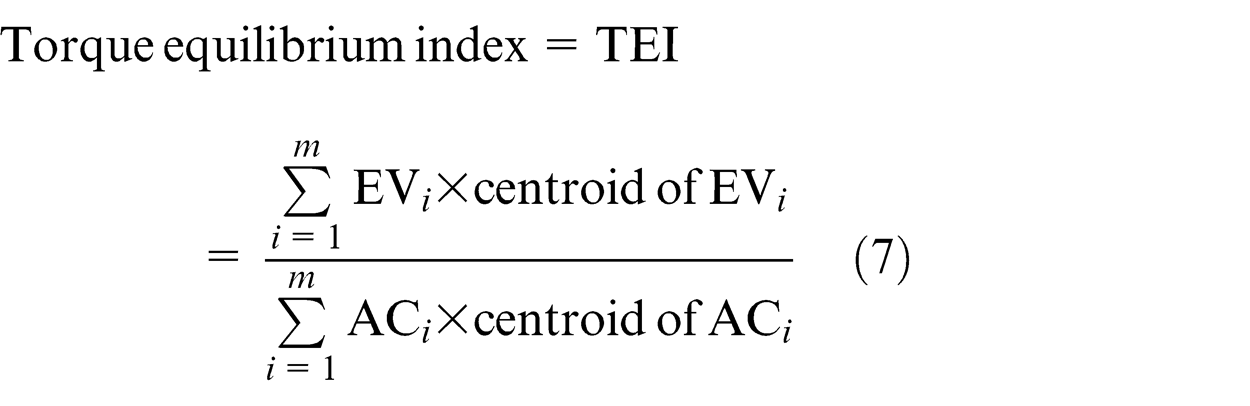
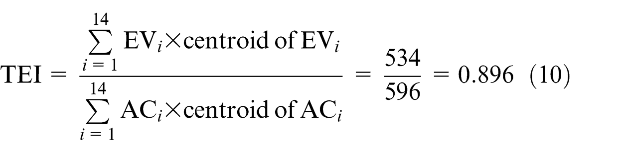
If CPI and Torque Equilibrium Index (TEI) indices are equal to 1, the project is in financial equilibrium. Otherwise, instability should be compensated in future by adding corresponding values (EV and AC) or force. The amount of acting forces (EV and AC) is determined by considering force equilibrium (equation (4)); however, the location of forces is determined by considering torque equilibrium (equation (5)). Thus, after determining the amount of forces (EV and AC) at next time periods, new acting forces should apply in a position that torque equilibrium condition is established.

In this stage, there are many choices for adding value or money (new acting forces) in different periods which optimization methods can use for finding the best condition according to the managerial points of view. Research methodology is shown in Figure 2.

Figure 2.

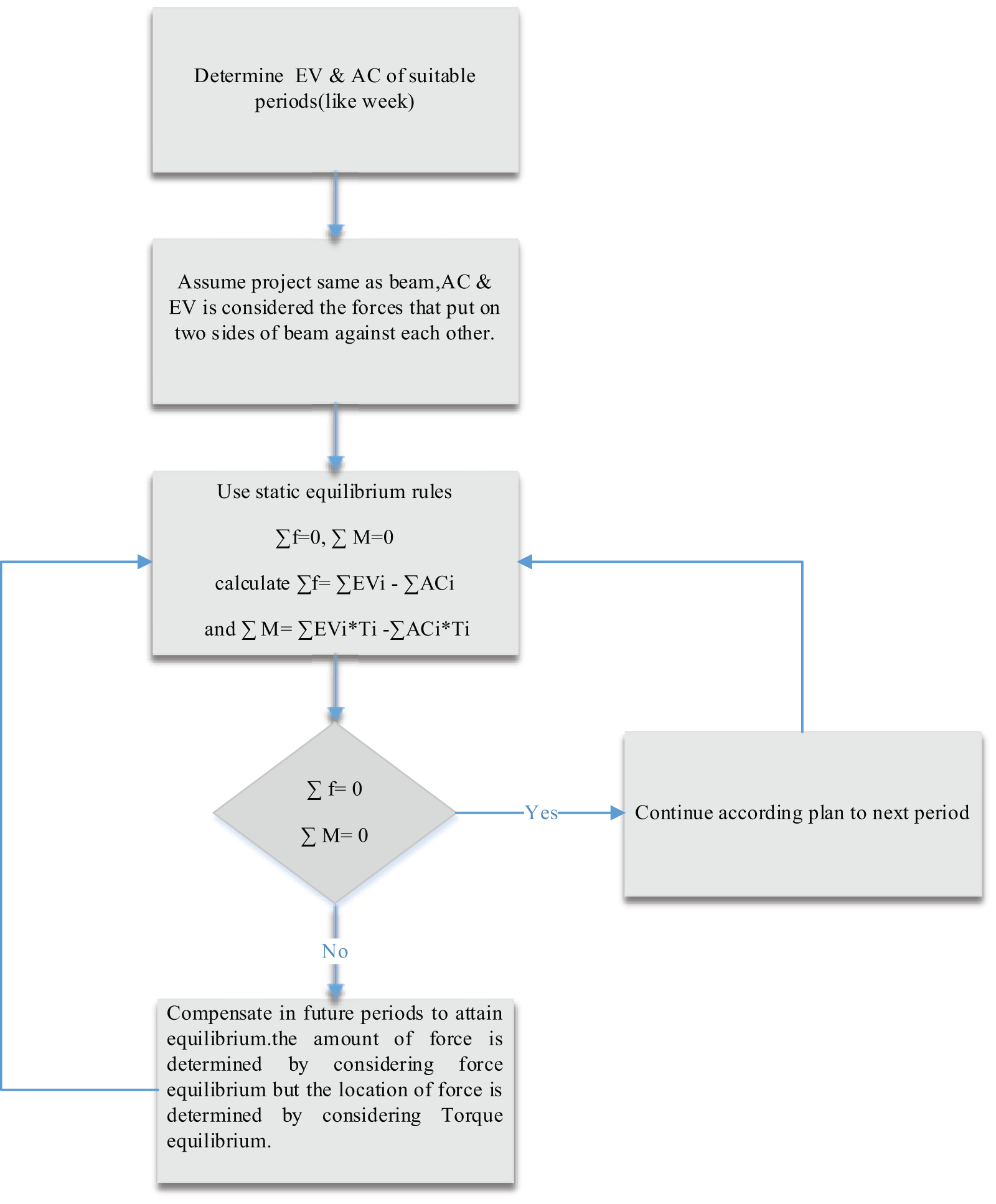
Research methodology.

Case study

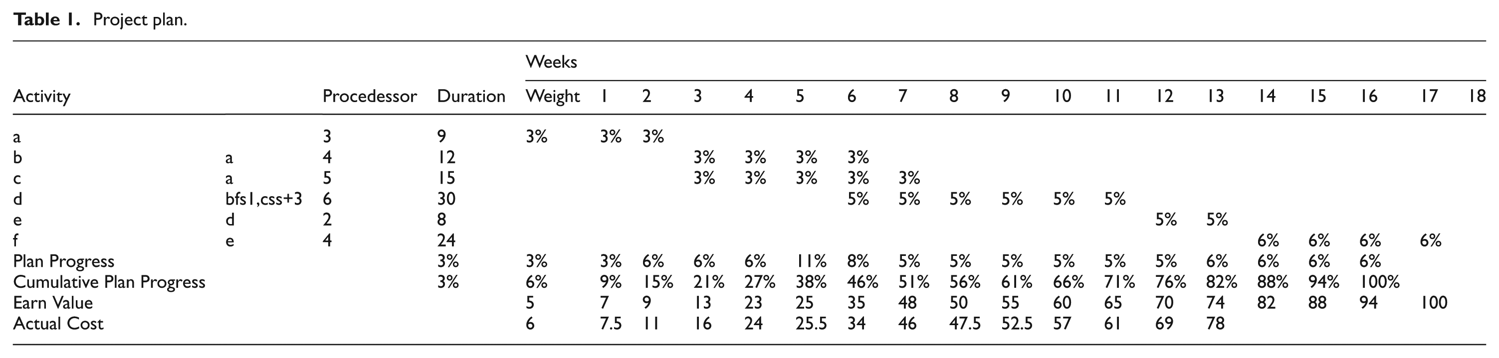
By using a case study, the new methodology is examined. In Table 1, project plan is shown. This project shall be completed in 18 weeks and the current cut-off date is at week 14. Budget at completion (BAC) is 100 monetary units. The project consists of six activities. Duration, predecessor and weight factors related to activities are shown in Table 1. Given the project data, EV and CPI have been calculated till week 14. Actual and planned progress is calculated weekly through cumulative basis. Financial system of the project is considered as a beam, and AC and EV at each week are assumed as distributed loads which act on two sides of the beam against each other; time interval (week) is considered as distance (X) in project, and because the project is in week 14, beam length is 14 m. For example, in first week, EV = 5 and AC = 6 which are applied as distributed loads on two sides of the beam (Figure 3). For beam equilibrium calculations, the distributed loads can turn to concentrated loads. Free-body diagram for the project with concentrated loads is shown in Figure 4. For every week, distributed loads are rectangular. The magnitude of the resultant load (concentrated load) for each week is equivalent to the area under the distributed load, and therefore, the location of the resultant force is at the center of the distributed load. For equilibrium, equations (4) and (5) must be established. In the project, $\sum F=0$ is equivalent to $\sum \mathrm{EV}-\mathrm{AC}=0$ . With regard to this explanation, calculation of resultant force is summarized in Table 2.

Table 1.

Project plan.

				Weeks
Activity		Procedessor	Duration	Weight	1	2	3	4	5	6	7	8	9	10	11	12	13	14	15	16	17	18
a		3	9	3%	3%	3%
b	a	4	12				3%	3%	3%	3%
c	a	5	15				3%	3%	3%	3%	3%
d	bfs1,css+3	6	30							5%	5%	5%	5%	5%	5%
e	d	2	8													5%	5%
f	e	4	24															6%	6%	6%	6%
Plan Progress			3%	3%	3%	6%	6%	6%	11%	8%	5%	5%	5%	5%	5%	5%	6%	6%	6%	6%
Cumulative Plan Progress			3%	6%	9%	15%	21%	27%	38%	46%	51%	56%	61%	66%	71%	76%	82%	88%	94%	100%
Earn Value				5	7	9	13	23	25	35	48	50	55	60	65	70	74	82	88	94	100
Actual Cost				6	7.5	11	16	24	25.5	34	46	47.5	52.5	57	61	69	78

Figure 3.

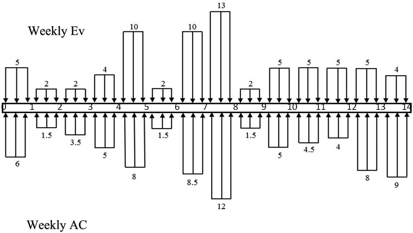
Free-body diagram for project with distributed load.

Figure 4.

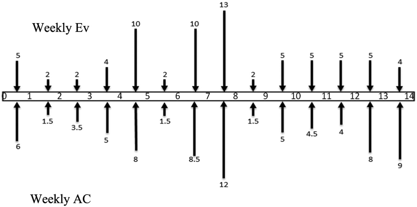
Free-body diagram for project with concentrated loads.

Figure 5.

Project bending moment diagram.

Table 2.

Project equilibrium calculations from 1st to 14th week.

Week	1	2	3	4	5	6	7	8	9	10	11	12	13	14	Sum
Centroid	0.5	1.5	2.5	3.5	4.5	5.5	6.5	7.5	8.5	9.5	10.5	11.5	12.5	13.5
Weekly EV	5	2	2	4	10	2	10	13	2	5	5	5	5	4	74
Weekly EV × centroid	2.5	3	5	14	45	11	65	97.5	17	47.5	52.5	57.5	62.5	54	534
Cumulative weekly EV × centroid	2.5	5.5	10.5	24.5	69.5	80.5	145.5	243	260	307.5	360	417.5	480	534
Weekly AC	6	1.5	3.5	5	8	1.5	8.5	12	1.5	5	4.5	4	8	9	78
Weekly AC × centroid	3	2.25	8.75	17.5	36	8.25	55.25	90	12.75	47.5	47.25	46	100	121.5	596
Cumulative weekly AC × centroid	3	5.25	14	31.5	67.5	75.75	131	221	233.8	281.3	328.5	374.5	474.5	596

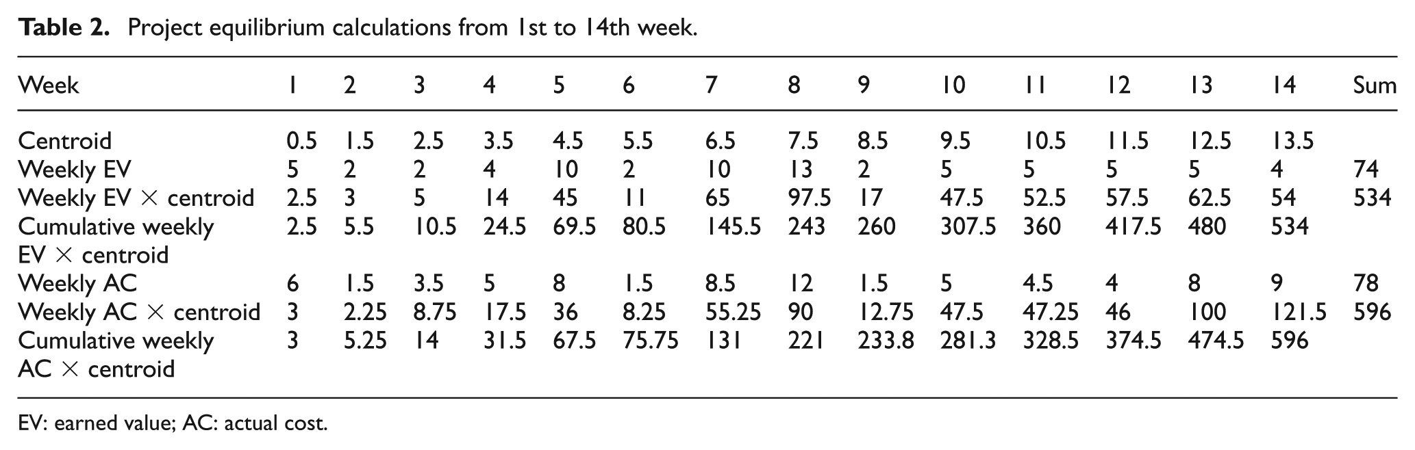
EV: earned value; AC: actual cost.

Regarding Table 2, it is obvious that force and torque equilibrium are not established in week 14. To reach force equilibrium, 4 monetary units must be added to the project

$${\displaystyle \sum _{i=1}^m}\mathrm{EV}-{\displaystyle \sum _{i=1}^m}{\mathrm{AC}}_i=74-78=-4$$

(8)

$${\displaystyle \sum _{i=1}^{14}}{\mathrm{EV}}_i\times \mathrm{centroid}\mathrm{of}{\mathrm{EV}}_i-{\displaystyle \sum _{i=1}^{14}}{\mathrm{AC}}_i\times \mathrm{centroid}\mathrm{of}{\mathrm{AC}}_i=534-596=-62$$

(9)

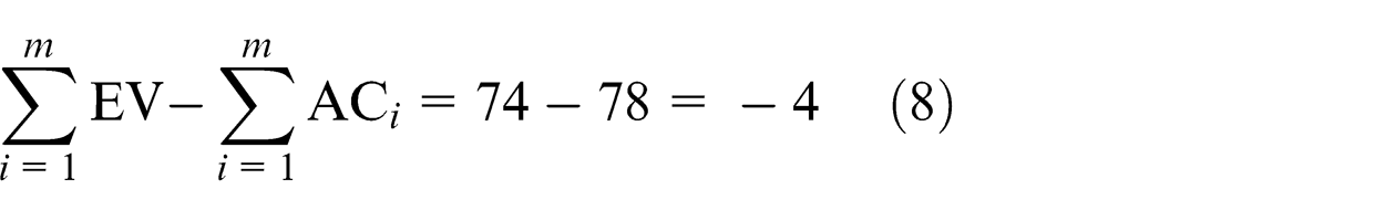
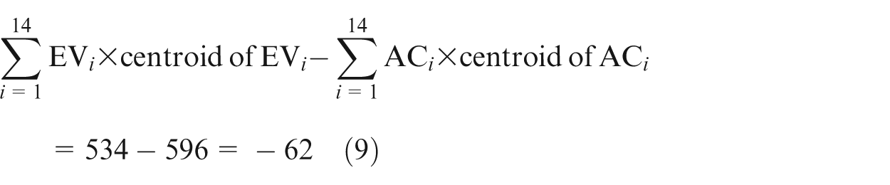
Because two indices are not equal to 0, the project is not in financial equilibrium. Then, TEI is equal to

$$\mathrm{TEI}=\frac{{\displaystyle \sum _{i=1}^{14}}{\mathrm{EV}}_i\times \mathrm{centroid}\mathrm{of}{\mathrm{EV}}_i}{{\displaystyle \sum _{i=1}^{14}}{\mathrm{AC}}_i\times \mathrm{centroid}\mathrm{of}{\mathrm{AC}}_i}=\frac{534}{596}=0.896$$

(10)

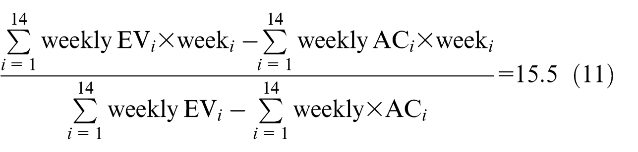
In addition, to reach torque equilibrium, the 4 monetary units can be added in 16th week according to equation (5) and the following calculation

$$\frac{{\displaystyle \sum _{i=1}^{14}}\mathrm{weekly}{\mathrm{EV}}_i\times {\mathrm{week}}_i-{\displaystyle \sum _{i=1}^{14}}\mathrm{weekly}{\mathrm{AC}}_i\times {\mathrm{week}}_i}{{\displaystyle \sum _{i=1}^{14}}\mathrm{weekly}{\mathrm{EV}}_i-{\displaystyle \sum _{i=1}^{14}}\mathrm{weekly}\times {\mathrm{AC}}_i}=15.5$$

(11)

However is not rationale that 4 monetary units to be added (injected) at one week (week 16) because of high pressure to earn more EV. Therefore, 4 monetary units should be distributed in the remaining weeks until the end of the project. The monetary units can be distributed in different situations such that mathematical methods can help to calculate applied load to reach equilibrium or optimization methods can help to optimize cost at this step.

For example, one of the situations to establish equilibrium is explained in the following. With regard to Table 1, planned progress in the last 4 weeks is equal to 6% per week. In addition, project has 2% delay than the pre-determined planned progress (in week 14), and this delay must be compensated on the remaining weeks; in other words, we can compensate this delay 0.5% per week.

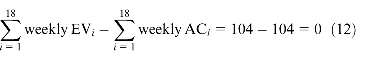
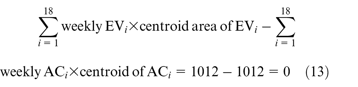
The difference between AC and EV is 4 units. Then, 1.5 monetary units should be compensated in 15th and 16th weeks and 0.5 monetary units in 17th and 18th weeks. This satisfies force and torque equilibrium.

As can be seen in Table 3, the project reaches full equilibrium condition at the completion

$${\displaystyle \sum _{i=1}^{18}}\mathrm{weekly}{\mathrm{EV}}_i-{\displaystyle \sum _{i=1}^{18}}\mathrm{weekly}{\mathrm{AC}}_i=104-104=0$$

(12)

$${\displaystyle \sum _{i=1}^{18}}\mathrm{weekly}{\mathrm{EV}}_i\times \mathrm{centroid}\mathrm{area}\mathrm{of}{\mathrm{EV}}_i-{\displaystyle \sum _{i=1}^{18}}\mathrm{weekly}{\mathrm{AC}}_i\times \mathrm{centroid}\mathrm{of}{\mathrm{AC}}_i=1012-1012=0$$

(13)

Table 3.

EV and AC from 15th to 18th week.

Week	15	16	17	18	Sum of 18 weeks
Centroid	14.5	15.5	16.5	17.5
Weekly EV	8	8	7	7	104
Weekly EV × centroid	116	124	115.5	122.5	1012
Cumulative weekly EV × centroid	650	774	889.5	1012
Weekly AC	6.5	6.5	6.5	6.5	104
Weekly AC × centroid of area	94.25	100.75	107.25	113.8	1012
Cumulative weekly AC × centroid	690.25	791	898.25	1012

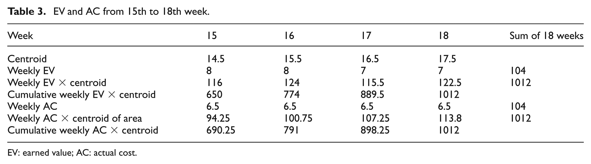
EV: earned value; AC: actual cost.

Reaching equilibrium situation in all weeks is difficult; however, it is necessary to reach equilibrium at the end of the project and specific cut-off dates. Finally, we can draw shear force and bending moment diagrams and study these diagrams. The relationship between bending moment and shear force is presented

$$\frac{\mathrm{dM}}{\mathrm{dX}}=V$$

(14)

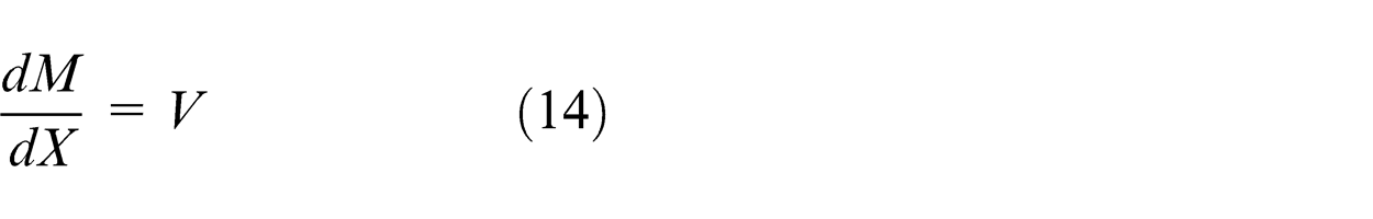
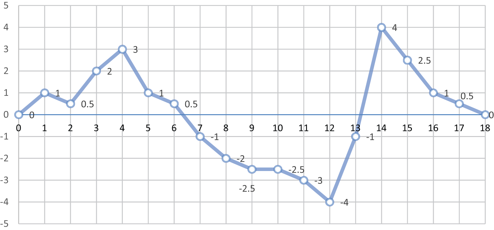
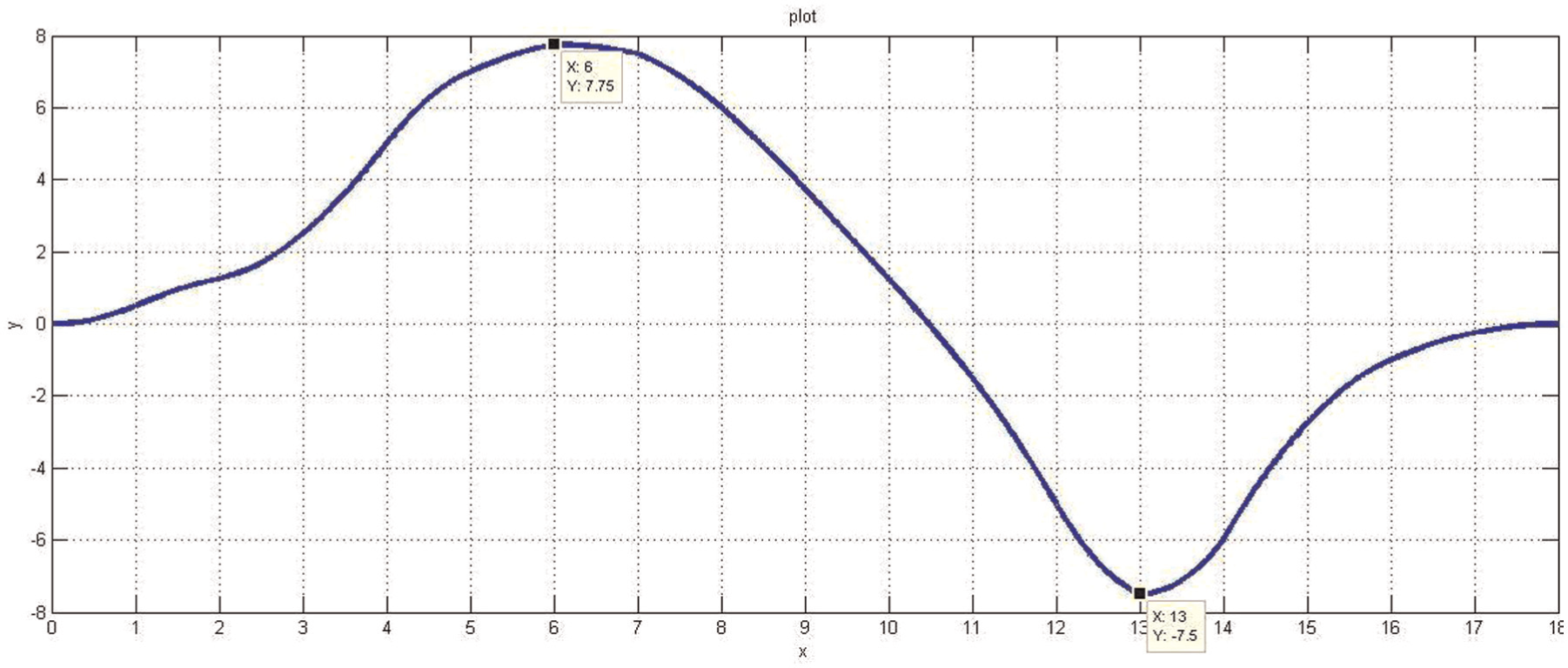
Equation (14) is used to draw bending moment diagram. Bending moment diagram is shown in Figure 6. As seen, there are sharp fluctuations in Figure 6, which represent the large imbalance in the financial status of the project. At the beginning, AC is greater than EV (CPI < 1), and the diagram shows an increasing trend till sixth week. Sixth week is critical and the most financial pressure is incurred on the project, and the project may fail in case of inaccessibility to potential fund resources. After passing 6th week, the project has decreasing trend till 13th week. In reality, it has low possibility that CPI > 1, but in this case it was different, and decreasing trend between 6 and 13 weeks happens due to CPI > 1. Then, after 13 weeks, the project has an increasing trend. Of course, 15–18 weeks are related to plan for reaching equilibrium condition. As observed, at week 18, EV = AC as well as bending moment is equal to 0.

Figure 6.

Project shear force diagram.

In reality, shear force is AC minus EV at each period, and it represents the conformity between EV and AC during project execution. Through an ideal condition, this diagram is a line which coincides on horizon axis, and by increasing the area under curve, instability will increase, as well as when this line is always on the top (it occurs when BAC estimation is wrong) or bottom of the horizon axis, the situation is more critical. Bending moment diagram can be applied to quantify the amount of instability; in other words, in this diagram, the area under curve is shear force (Figure 5). In maximum points, the most pressure is incurred on the contractor, and as mentioned, if the contractor cannot tolerate this financial pressure, it can lead to project failure, and after maximum points, financial pressure (due to project cost) will gradually decrease. If BAC estimation is correct, in minimum points, the contractor falls at the best financial status.

Conclusion

CPI measure cannot individually represent shortages in financial status of a project. Using the rules of beam equilibrium, a better understanding for overcoming the shortages can be made. Also, EV and AC shortages are recognized, and using bending moment equilibrium, the exact time for adding the monetary units to the project is determined. Therefore, managers should try to establish financial equilibrium in projects. Otherwise, they may tolerate high financial pressure and in the maximum bending moment may face financial shortages, and it can lead to project failure. Further research can be done on applying reliability-based functions emerging with mechanical equilibrium condition through project cost management system.