
Abstract
Mechanical micromachining is a very flexible and widely exploited process, but its knowledge should still be improved since several incompletely explained phenomena affect the microscale chip removal. Several models have been developed to describe the machining process, but only some of them consider a rounded edge tool, which is a typical condition in micromachining. Among these models, the Waldorf's slip-line field model for the macroscale allows to separately evaluate shearing and ploughing force components in orthogonal cutting conditions; therefore, it is suitable to predict cutting forces when a large ploughing action occurs, as in micromachining. This study aims at demonstrating how this model is suitable also for micromachining conditions. To achieve this goal, a clear and repeatable procedure has been developed for objectively validating its force prediction performance at low uncut chip thickness (less than 50 μm) and relatively higher cutting edge radius. The proposed procedure makes the model generally applicable after a suitable and non-extensive calibration campaign. This article shows how calibration experiments can be selected among the available cutting trial database based on the model force prediction capability. Final validation experiments have been used to show how the model is robust to a cutting speed variation even if the cutting speed is not among the model quantities. A suitable set-up, especially designed for microturning conditions, has been used to measure forces and chip thickness. Tests have been performed on 6082-T6 Aluminum alloy with different cutting speeds and different ratios between uncut chip thickness and cutting edge radius.
Introduction
Among the different available processes, micro mechanical machining is one of the most flexible and widely exploited ones, even if its characterizing phenomena are still not well understood and controlled; basic knowledge about the physical phenomena1,2 should still be improved and, in particular, the following scale effects need to be further studied:
If critical tool geometrical features, as the edge radius, assume the same magnitude order of the chip thickness, the tool effective rake angle gets highly negative, ploughing forces become more relevant than shearing forces and the cutting-specific energy gets higher.3,4
Chip removal becomes discontinuous since a minimum uncut chip thickness exists under which no material can be removed from the workpiece (minimum chip thickness effect).3–6
The workpiece material microstructure plays an important role on cutting forces, since the tool geometrical features tend to be comparable in size to the target material grains and make them vary with the grain orientation.7,8
A stable built-up edge, named “dead metal cap,” is claimed by some researchers to be always present when machining with an uncut chip thickness lower than the tool cutting edge radius.9–11
State of the art
Over the years, the chip removal process has been described by several models; Lee and Shaffer 12 first presented a model based on the so-called slip-line field theory, potentially able to predict also the ploughing effects. This is the main reason why slip-line field theory is the focus of this article.
The existing slip-line field models consider different tool shapes, which are mainly the following:
The typical microscale conditions can be better represented by taking into account a rounded tool shape. In fact, the cutting edge radius is always significant at this scale, due to current tool fabrication process capability that prevents it to be lower than typical chip thickness at the microscale. In recent years, many slip-line field models have been specifically developed for the microscale9,10,21–29 and all of them consider a rounded tool edge.
The above-cited models can be divided into two groups taking into account the applied modeling approach:
The assumption of a stable built-up edge (according to experimental findings of Kountanya and Endres 11 ) was made by Waldorf et al.,9,10 Liu et al.,23–25 Karpat and Özel, 26 Yoon and Ehmann 27 and Ozturk and Altan. 29
The assumption of a separation point on the tool edge diverting the material flow was made by Fang21,22 and Jin and Altintas. 28
Among the first model group, the study by Waldorf et al.9,10 presented a slip-line field model consisting of three shear zones, which is able to predict also the ploughing force components. The authors made the assumptions of constant friction factor and rigid, perfectly plastic material (i.e. the shear flow stress only depends on the machined material but not on strain, strain rate or temperature). The authors validated their model by performing orthogonal turning tests on Al 6061-T6. 9
In their study, Liu et al.23–25 proposed a slip-line field similar to the Fang’s21,22 one but considering only slip-lines necessary for cutting force calculations. Moreover, the authors took into account the dead metal cap presence and introduced the effective rake angle in the model as a function of the uncut chip thickness. 33
In their article, Karpat and Özel 26 proposed a model derived from Waldorf’s one in which the friction factor was calculated based on cutting forces and acquired chip geometry. The authors performed a finite element analysis, applying the Johnson–Cook model, to evaluate the shear flow stress. They also carried out orthogonal turning tests on AISI 4340 steel with an uncut chip thickness of 100, 125 and 150 μm (corresponding to a normalized uncut chip thickness t c/r e between 2.5 and 3.75, since the used cutting edge radii were 40 and 50 μm) and a cutting speed of 125 and 175 m/min.
Yoon and Ehmann 27 designed a slip-line field model including the minimum chip thickness effect and the effective rake angle; they also supposed the friction factor to be constant. The model was validated by means of microturning tests on 260 brass alloy (CuZn30) with an uncut chip thickness ranging from 1 to 13 μm and a cutting edge radius of 5 μm.
In their study, Ozturk and Altan 29 presented a slip-line field composed by eight shear regions and including a dead metal cap, under the assumptions of constant friction factor and rigid, perfectly plastic material. In order to validate the model, some orthogonal cutting experiments were performed on 260 brass alloy (CuZn30) using tools with a cutting edge radius of 50, 100 and 150 μm; the uncut chip thickness was equal to 50, 100 and 150 μm (hence the normalized uncut chip thickness t c/r e ranged from 0.33 to 3) and the selected cutting speeds were 0.25, 0.50 and 0.75 m/min in order to avoid thermal effects. This article also shows some chip micrographs obtained by a quick stop device successfully operating up to a maximum cutting speed of 17.5 m/min.
Among the second model group, the model by Fang21,22 is composed by 27 slip-line subregions and allows to estimate also the ploughing force components. The mathematical formulation of this model is based on Dewhurst and Collins matrix technique15,34 and carries out a non-unique solution. The predicted forces were compared with experimental observations coming from past works by other authors.
Jin and Altintas 28 designed a model that divides the material deformation region into three main zones; they applied the Johnson–Cook constitutive model to obtain the shear flow stress and the hydrostatic pressure as functions of strain, strain rate and temperature. The authors validated their model by carrying out turning experiments on 260 brass alloy (CuZn30) using a tool with a 20-μm cutting edge radius and a cutting speed between 150 and 350 m/min. The selected uncut chip thickness values were between 15 and 80 μm, in order to obtain a ratio with the cutting edge radius ranging from 0.75 to 4.
These orthogonal cutting models are useful to describe the chip formation process and, hence, to improve the knowledge on the machining process. Orthogonal cutting models based on the slip-line theory can also be used for other purposes, for example, some researchers developed milling models based on an orthogonal cutting slip-line field that is linked to the milling process by a proper chip thickness analytical function. This approach was used in the studies of Jun et al.23,24 and Altintas and Jin, 35 which are, respectively, based on the slip-line field models by Waldorf et al. 9 and Jin and Altintas. 28
Objectives
As discussed for the state of the art, an experimental validation of models presented in the literature has just been made in some of the analyzed articles.9,10,26–29 This article focuses on Waldorf’s model 9 with the purpose to validate it in the micromachining field.
This model has been selected since it is simple, it has only a few parameters to experimentally calibrate (no finite element method (FEM) analysis is needed) and, at the same time, it allows to evaluate cutting forces when a strong ploughing occurs (i.e. when the uncut chip thickness is lower than the tool edge radius), that is, in the typical micromachining conditions. Moreover, Waldorf et al. 10 showed how models including a stable built-up edge have a better prediction performance than models assuming the material separation at a certain point on the tool cutting edge.
After taking the Waldorf model9,10 as reference, this study has developed a repeatable procedure to calibrate it for a specific target material by means of a suitable restricted set of experiments. 36 Such a calibration procedure allows to make the model a useful tool to predict the cutting and thrust forces in different conditions of feed and cutting speed that are significant for the microfield and outside the calibration window. This study demonstrates this result for both the original Waldorf model and for a modified version considering the effective rake angle. 36 An objective comparison between performances of the two versions is also presented to confirm the usefulness of the effective rake angle introduction. 36 Introducing the effective rake angle allows to account for typical low chip thickness effects on microcutting, which make the rake angle strongly negative, the ploughing forces sometimes more relevant than shearing forces and the specific cutting energy extremely high. Moreover, the effective rake angle introduction allows modeling a dead metal cap size changing with the uncut chip thickness. Finally, a model validation has been presented where cutting speed has been varied comparing to calibration experiments in order to show how the model is robust to a cutting speed variation.
Waldorf’s slip-line field model
Waldorf et al.9,10 developed a slip-line field model for the orthogonal cutting condition that is able to predict the cutting and thrust force components, also considering their shear and ploughing portion. Figure 1 depicts this field that partly derives from previous slip-line fields in the literature. In particular, it resembles the model developed by Shi and Ramalingam 32 for cutting with flank wear, that, in turn, has been developed based on a slip-line solution for orthogonal cutting proposed by Kudo. 14
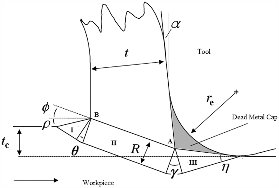
Slip-line field proposed by Waldorf.
The slip-line field proposed by Waldorf consists of three regions of rigid material motion:
The first region (I in Figure 1) is a pre-flow zone where a material raising takes place due to compressive stresses; the prow angle (ρ in Figure 1) accounts for this effect.
The second region (II in Figure 1) corresponds to the traditional “primary shear zone” that is defined by the shear angle (
The third region (III in Figure 1) is the “tertiary shear zone,” which is close to the dead metal cap. Its dimensions depend on the friction conditions at the tool–chip interface.
The “secondary shear zone,” where the tool rake face gets in contact with the chip, is not considered in the Waldorf model.
Some of the model parameters are immediately available once the experimental conditions are defined, that is, they are defined outside the model and do not need to be calibrated:
m (adhesive friction factor, that is, the ratio between shear and flow stress) = 0.99, as stated by Waldorf et al. 9
r e (cutting edge radius) = 35 μm and α (rake angle) = 16°, obtained by measurements made on the insert used in this article (see section “Experiment description”) by an Alicona Infinite Focus optical three-dimensional (3D) measuring system.
t c (uncut chip thickness) equal to the feed f, since orthogonal cutting hypotheses are satisfied in microturning experiments (see section “Experiment description”).
w (width of cut) = 0.73 mm, obtained as the mean of measurements made on the workpieces by a Zeiss Prismo 5 VAST MPS HTG Coordinate Measuring Machine.
Only three model input parameters (
Calibration and validation experimental database
Experimental design
A factorial experiment (whose factors are summarized in Table 1) has been designed in order to build an experimental database useful to calibrate and validate the Waldorf model, in case of both the original model version9,10 and the Waldorf model considering the effective rake angle.
Experimental design factors.
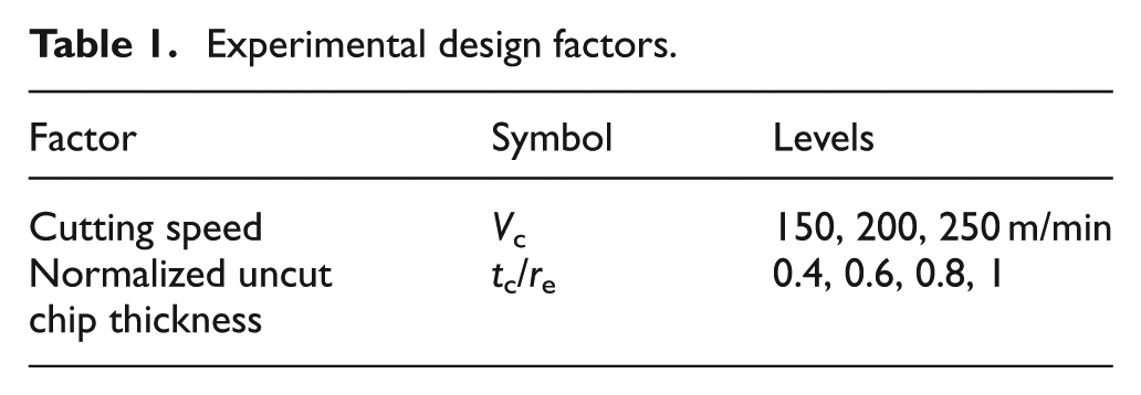
The cutting speed factor varies on three levels: 150, 200 and 250 m/min. Such values have been selected in a range where cutting takes place satisfactorily (no vibrations, no burrs, good surface finish) according to preliminary tests. The considered normalized uncut chip thickness levels are four: 0.4, 0.6, 0.8 and 1, corresponding, respectively, to an uncut chip thickness of 14, 21, 28 and 35 μm. These values have been selected in order to ensure a regular chip formation by staying immediately above the commonly accepted value of minimum uncut chip thickness, equal to 0.3/0.4 r e. 4
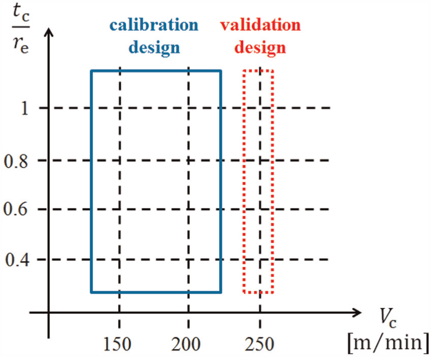
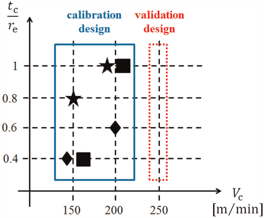
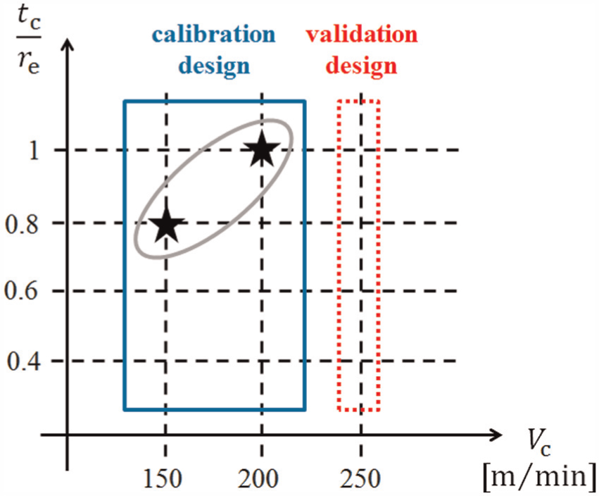
Four replicates have been carried out for each factor’s combination; hence, the experimental design (Figure 2) consists of 48 runs, which have been completely randomized.
Experimental database.
The whole experimental database has been divided into two parts: the calibration design (blue solid box in Figure 2) provides the experimental condition sets for the model calibration (see section “Model calibration conditions' selection”), while the validation design (red dotted box in Figure 2) is used to validate the model prediction performance (see section “Model validation”).
The cutting speed is not a model input parameter; however, it is known that the cutting speed affects the material properties (e.g. a cutting speed increase causes a softening effect), hence the selected model has been validated also for a different cutting speed level in order to prove its robustness. It seems reasonable not to exceed with the cutting speed values since they are typically low in micromachining.
Experiment description
Microturning operations have been performed by means of a suitable set-up designed to be used on the Kern EVO ultra precision five-axis machining center available at the “MI_crolab” of Dipartimento di Meccanica of Politecnico di Milano (nominal positioning tolerance = ±1 μm, precision on the workpiece = ±2 μm). A Kistler 9257BA triaxial piezoelectric load cell (D in Figure 3) has been employed to measure cutting forces during each test.
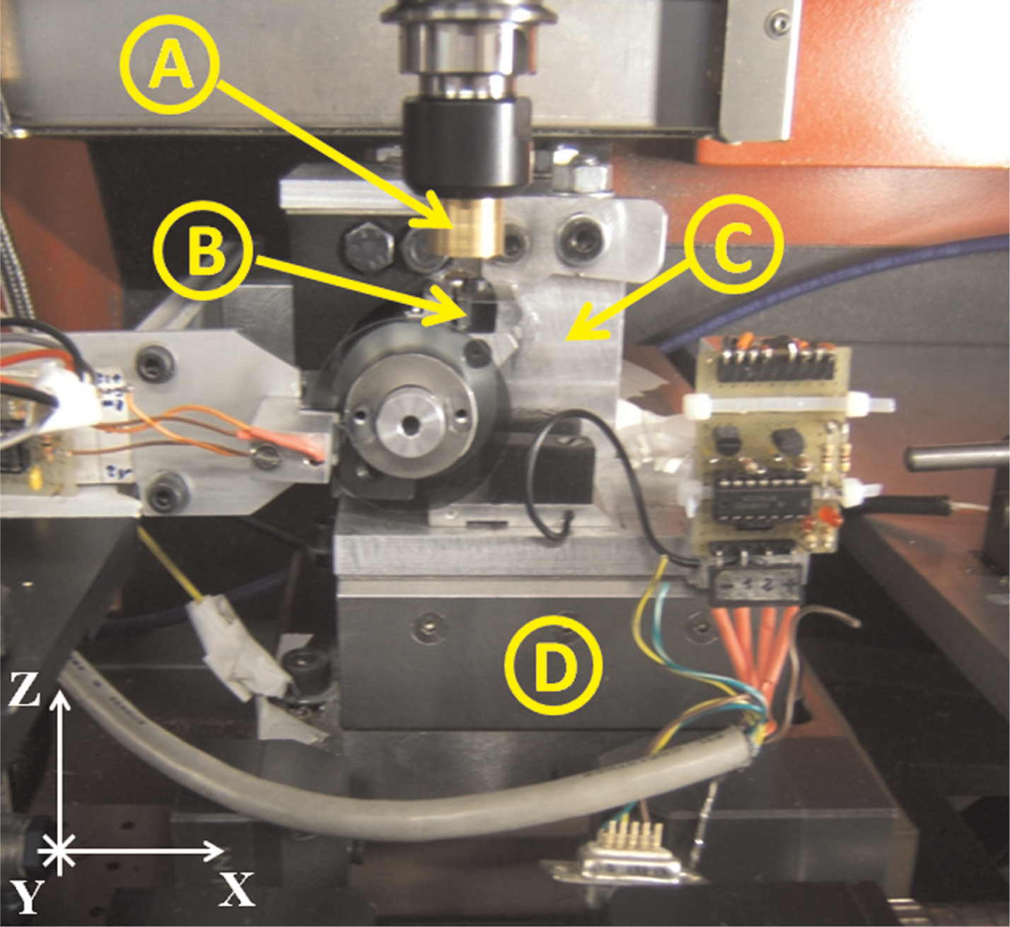
Microturning set-up (A = workpiece, B = tool, C = tool holder, D = load cell).
The orthogonal cutting condition (Figure 4) has been obtained by turning a thin-walled tubular workpiece (diameter = 15 mm, nominal wall thickness = 0.7 mm), mounted on the machine spindle (A in Figure 3) and moving at the cutting speed V c. The turning tool carrying out the operations (B in Figure 3) has been fixed to the machine table by a proper tool holder (C in Figure 3). Thanks to this set-up, the orthogonal cutting condition exists since the following hypotheses are satisfied: the cutting edge is perpendicular to the cutting speed and wider than the width of cut w (i.e. the chip has no constraints at its sides), the cutting speed has acceptable variations along the cutting edge and the uncut chip thickness t c is much lower than the width of cut w. Moreover, the uncut chip thickness t c can be considered equal to the actual feed f since the feed rate is negligible comparing to the cutting speed.
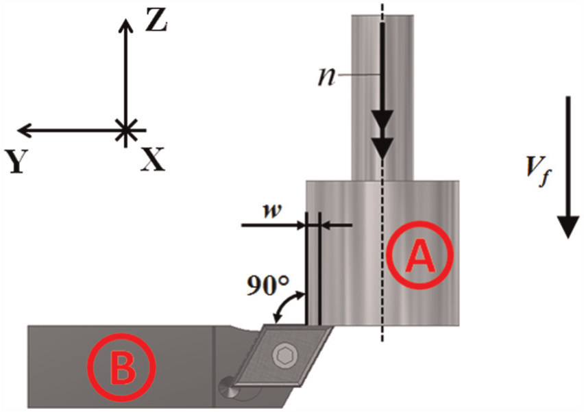
Orthogonal cutting operation sketch (A = workpiece, B = tool).
Each workpiece has been pre-machined on a traditional lathe and then measured on the Kern EVO by means of the Blum Micro Compact NT laser presetting system (accuracy: 1 μm) in order to detect possible errors. Diameter measurements on different workpiece—tool holder couples at different heights showed a maximum standard deviation σ = 7 μm including dimensional, fixturing and run-out errors. Such a deviation is acceptable for the presented experimentation.
The orthogonal cutting tests were carried out by means of a Sandvik DCMX 070202—WF1125 carbide insert (Figure 5); the insert main characteristics are listed in Table 2.
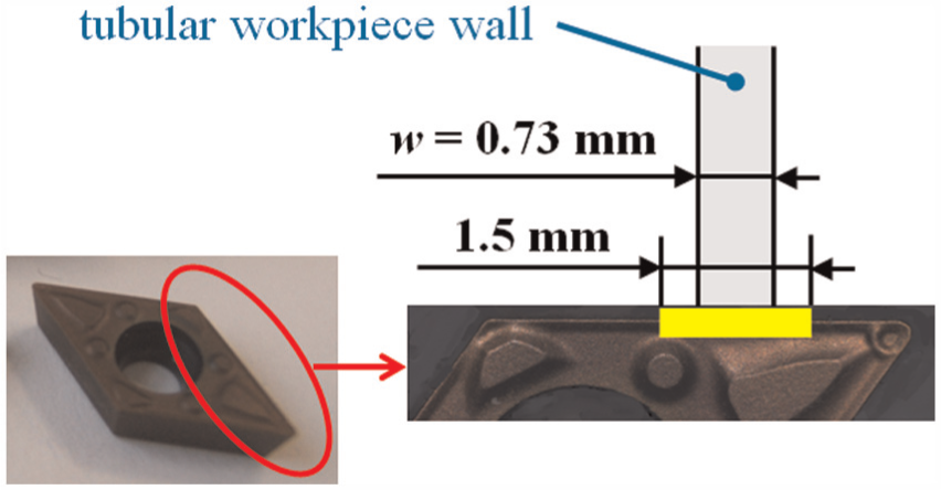
Sandvik DCMX 070202—WF1125 carbide insert.
Experimental design constant parameters.
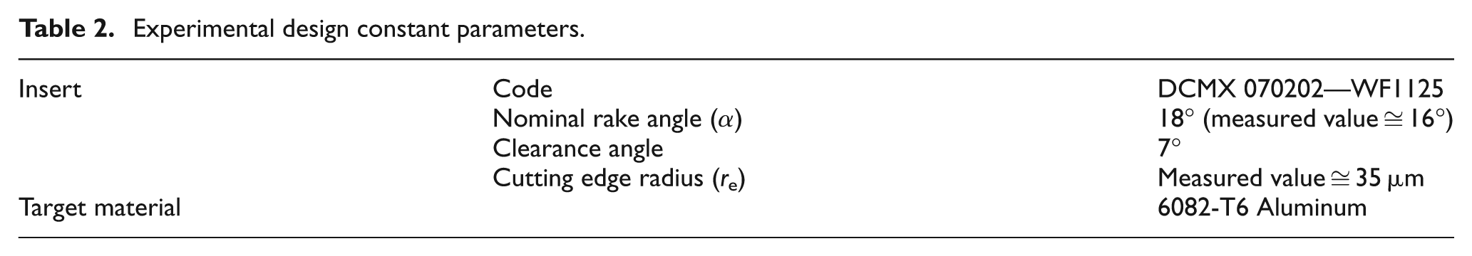
The tested target material is the 6082-T6 Aluminum alloy, whose measured hardness is 59 HRB. This material has been selected since it is the currently available aluminum alloy in the market similar to the Waldorf target material. 9
The cutting edge radius and the rake angle have been measured by means of an Alicona Infinite Focus optical 3D measuring system (measurement parameters: 10× magnification, exposure time = 40.1 ms, polarized light). The measured values are reported in Table 2. The cutting edge radius value (Figure 6) has been obtained by calculating the mean of measurements made in three different zones along the insert cutting edge over a 1.5-mm length (yellow line in Figure 5). The rake angle value cannot be shown in the profile of Figure 6 where no references are reported.
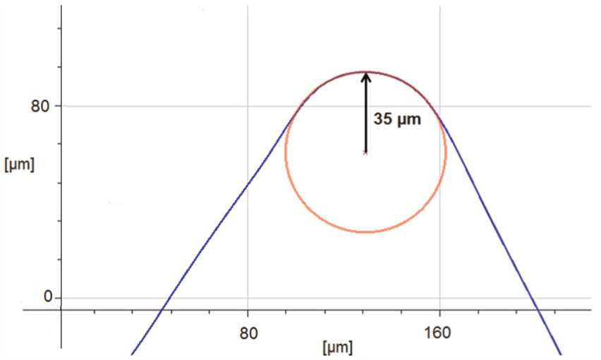
Tool cutting edge radius measurement carried out by Alicona Infinite Focus (mean profile along yellow line in Figure 5).
Moreover, Alicona Infinite Focus has been used to measure the chip thickness t directly on chips produced during each turning test. For each test, three chips have been measured three times over a very narrow band (white line in Figure 7) to have a nearly punctual measurement (measurement parameters: 5× magnification, exposure time = 300 ms, non-polarized light and ring light); the chip thickness value t is the nine measurements’ mean. Chip thickness has also been checked by means of a Microrep DMS 680 Universal Length Measuring System.
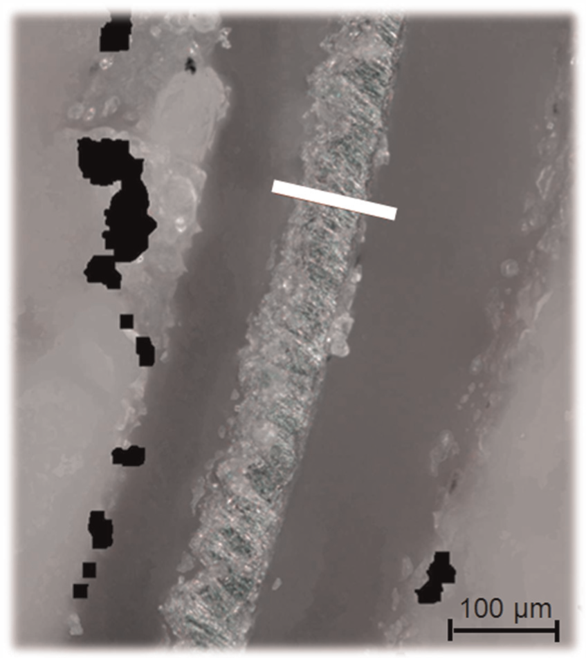
Chip thickness measurement by Alicona Infinite Focus.
Model calibration and force prediction procedure development
This study aims at demonstrating how the Waldorf’s model is suitable for micromachining conditions. In order to achieve this result, this article presents a clear and repeatable procedure for calibrating and applying a slip-line model to force prediction in the microscale. The analyzed literature lacks such a kind of procedure, making the model application very unstructured and leading to repeatability problems.
The scheme in Figure 8 summarizes this procedure: boxes contain the reference to the applied formulas or actions to perform, while the arrows have different meanings depending on their position (box top and left: resources and input; box bottom and right: output).
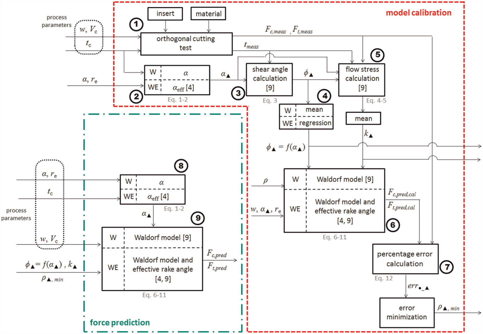
Calibration and force prediction procedure scheme.
The scheme in Figure 8 is divided into two main parts, one concerning the model calibration phase and the other concerning the model cutting force prediction phase. The whole procedure is applied to both the original Waldorf model and the Waldorf modified version considering the effective rake angle; since some quantities are different in the two cases, they have been indicated by the subscript ▴, assuming the value “W” for the Waldorf model or “WE” for the Waldorf model modified with the effective rake angle. The comparison between the two model versions is a secondary result of this study.
Model calibration
The actions in the part of Figure 8 named “model calibration” must be carried out prior to the model use, in order to calibrate it. The following part of this section describes the scheme of Figure 8 starting from box 1.
Box 1—orthogonal cutting test
Once the target material and the insert have been selected, some orthogonal cutting tests have to be performed with suitable process parameters. During the cutting tests, the cutting and thrust force components (respectively, F c and F t) have to be acquired to calculate their mean value (F c,meas, F t,meas). Moreover, the resulting chip thickness t has to be measured for each experiment (t meas). It has to be pointed out as F c,meas, F t,meas and t meas are vectors with lengths equal to the number of carried out calibration tests.
Box 2—rake angle
The rake angle α is equal to its nominal value when applying the W approach while it varies with the selected uncut chip thickness t c when applying the effective rake angle approach. The effective rake angle α eff (Figure 9) is introduced in the Waldorf slip-line field model to account for typical low chip thickness effects on microcutting, which make the ploughing forces increase as the uncut chip thickness decreases. In particular, the effective rake angle introduction allows to model a dead metal cap size changing with the uncut chip thickness.
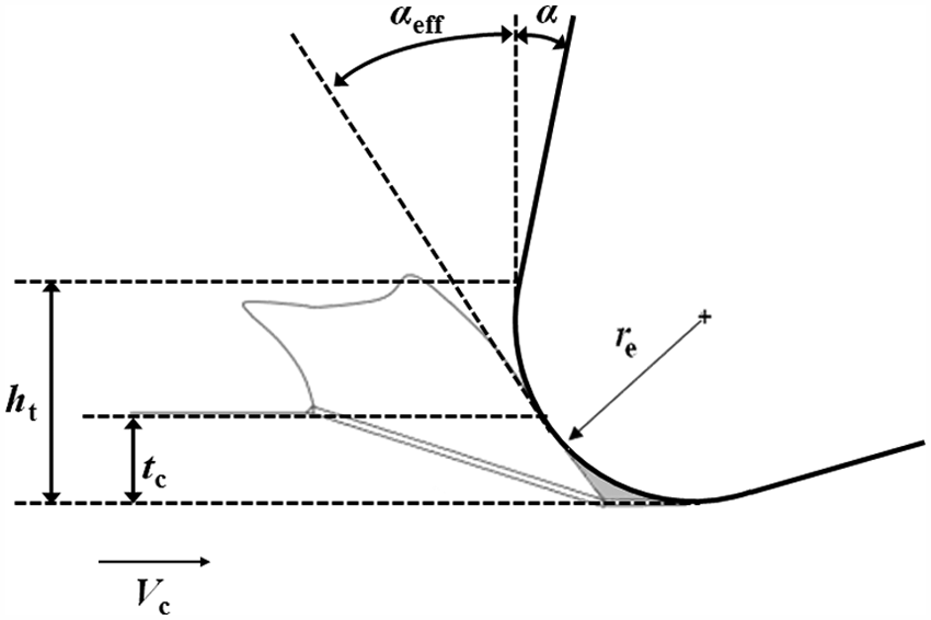
Effective rake angle.
Equation (1) defines the height h t of the tangency point between the tool rake surface and the cutting edge radius r e arc 4
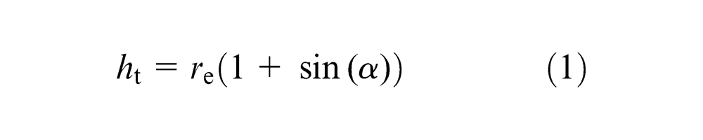
When the uncut chip thickness t c is lower than h t, the effective rake angle can be obtained as the inclination angle of the tangent to the cutter edge arc at the point corresponding to t c (equation (2))
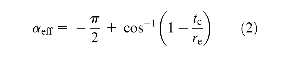
where t c/r e is named “normalized uncut chip thickness.” Otherwise, when the uncut chip thickness t c is higher than h t, the effective rake angle α eff is equal to the nominal rake angle α, as shown in Figure 10, where three different nominal rake angle values are considered as an example.
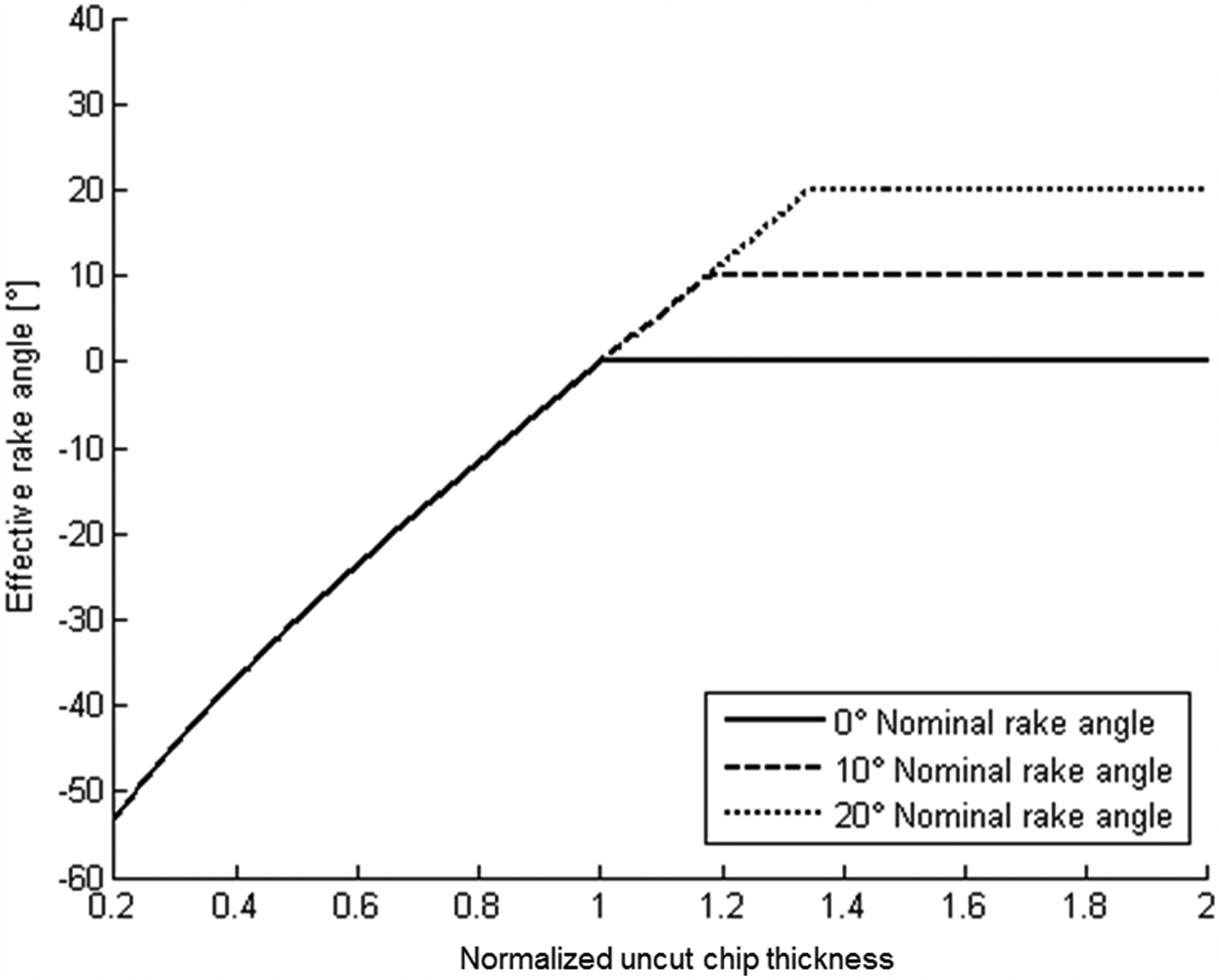
Relationship between the effective rake angle α eff and the normalized uncut chip thickness t c/r e.
Box 2 output (α ▴) is a vector with length equal to the number of carried out calibration tests but, when applying the W approach, it is composed by identical elements equal to the nominal rake angle value.
Box 3—shear angle (first step)
A relation based on the chip compression ratio
9
is applied to calculate the shear angle
Box 3 carries out a vector (
Box 4—shear angle (second step)
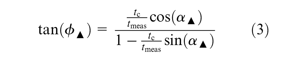
The tc
/tmeas
ratio can be assumed to be almost constant as observed from experimental data (Figure 11); therefore, the shear angle
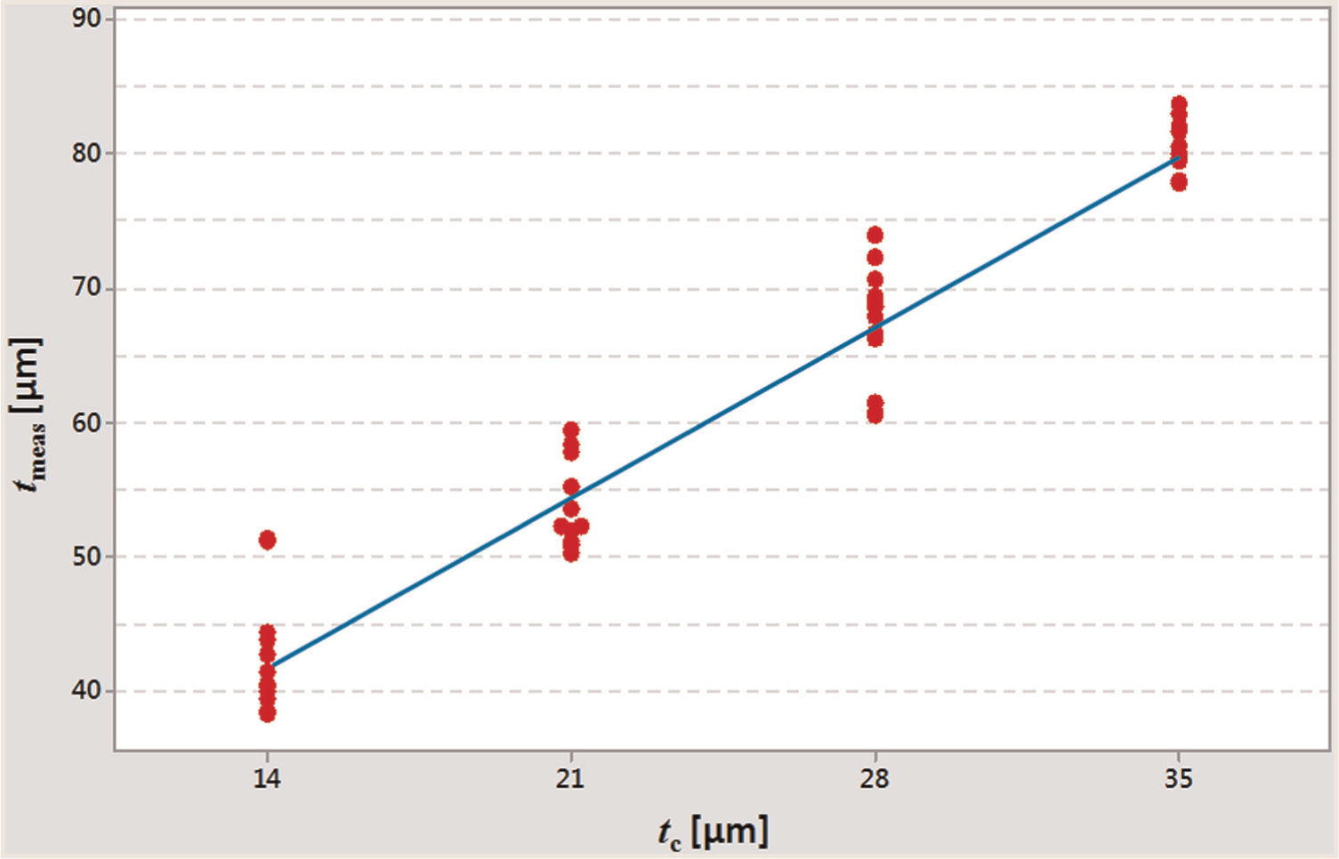
Relationship between measured chip thickness t meas and uncut chip thickness t c.
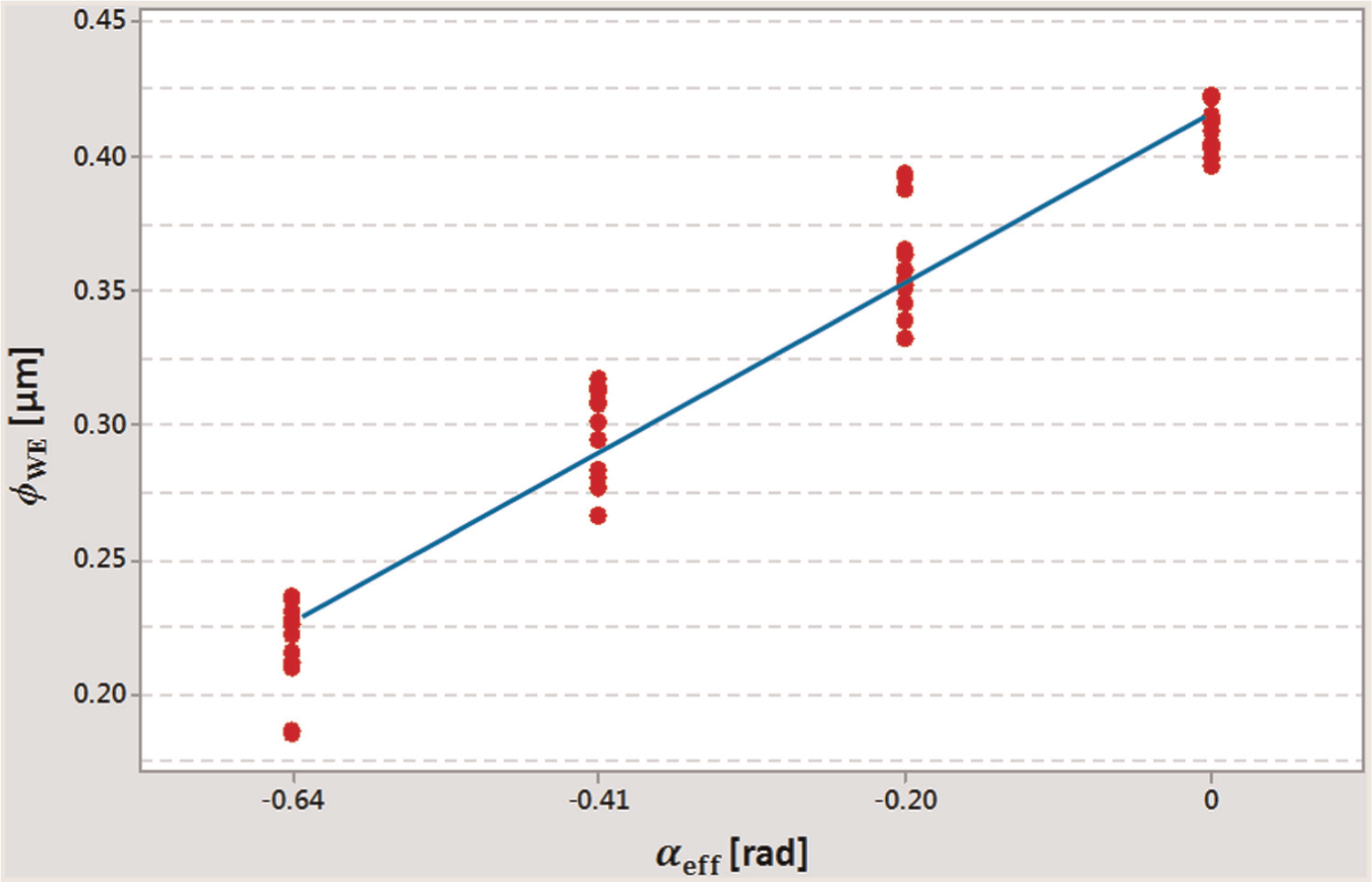
Relationship between shear angle
Figure 12 represents all the 48 experimental results making part of the experimental database carried out in this study (Table 1) in order to demonstrate the correctness of the described assumptions on the shear angle dependence from the rake angle and the chip thickness. The calibration procedure does not need such an amount of data to be effective, as it has been pointed out in section “Model calibration conditions' selection.”
Box 5—flow stress
The flow stress k for the considered target material is calculated for each cutting test by applying the following equation 9
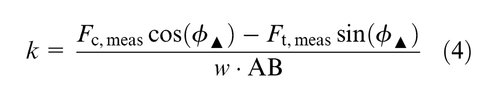
where the shear plane length is evaluated as follows 9

Since k is supposed to be independent from cutting parameters, the value to use as force prediction model input is obtained as the mean of calculated values for both the W and the WE approaches. For this reason, box 5 gives a scalar as output.
Equation (4) only works when the ploughing forces are negligible, that is, for higher values of normalized uncut chip thickness, which does not represent a typical microscale condition. 9 Since the proposed procedure is modular, each box can be changed independently from the others. In particular, the flow stress k could be calculated according to other methods, such as the Johnson–Cook model or the relationship between the flow stress and the microhardness. 37 This opportunity will be evaluated in future developments of this research.
Box 6—prow angle
Before using the model to predict cutting forces, also the prow angle ρ (Figure 1) has to be calibrated. In order to do that, F c and F t can be calculated for different ρ values based on the already obtained φ ▴ and k ▴ parameters.
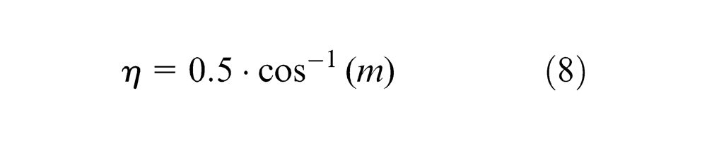
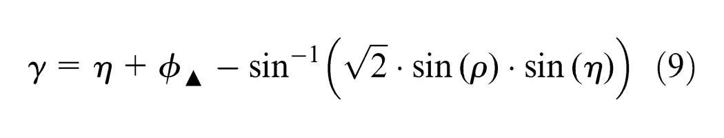
Box 6 applies the following equations (6)–(10), 9 where ρ is a vector of possible prow angle values (in this article, 15 values ranging from 0 to 0.7 rad with steps of 0.05 rad have been tested), and F c,pred,cal and F t,pred,cal are matrixes whose dimensions correspond to the number of carried out calibration tests and to the ρ vector length, respectively.
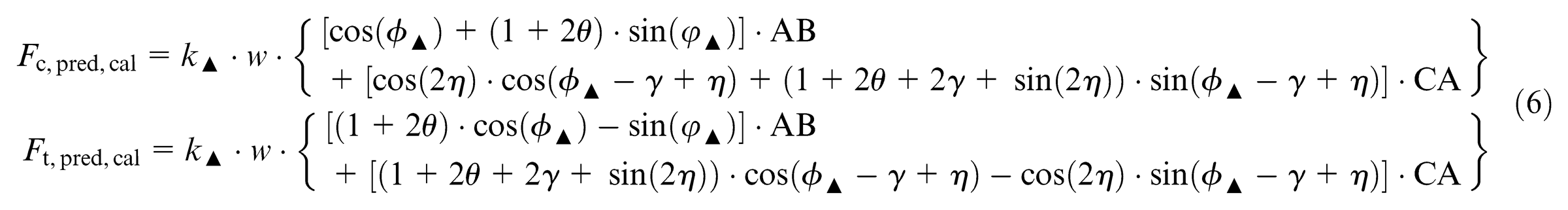
where


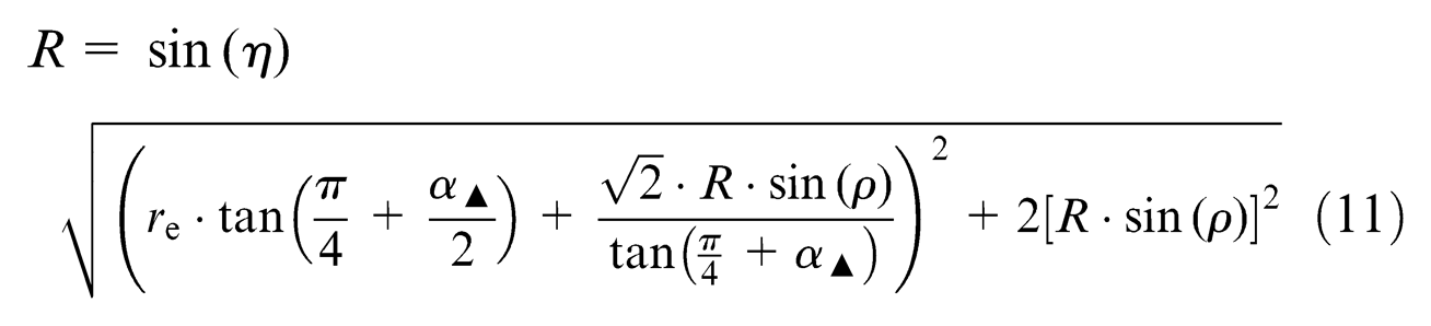
The radius R of the circular fan field centered in A (Figure 1) is obtained by solving equation (11) 9
Box 7—percentage error
The percentage errors between the force predicted values (F c,pred,cal and F t,pred,cal) and the measured mean values (F c,meas and F t,meas) can be calculated as follows
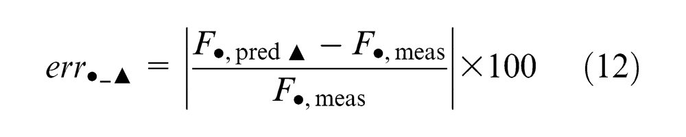
where • describes the force direction assuming the value “c” for cutting or “t” for thrust force.
Each
Force prediction
This section briefly explains the force prediction part of Figure 8 scheme. As it can be noted, it is composed of two boxes (boxes 8 and 9) that correspond, respectively, to boxes 2 and 6 of the “model calibration” part.
In particular, box 8 is completely identical to box 2 and calculates the rake angle according to both the W and the WE approaches. Box 9 is composed by the same equations of box 6; regarding its input, it receives φ▴ = f(α▴ ), k▴ and ρ ▴,min values from the calibration procedure and α▴ from box 8, where the model user has to provide α, r e and t c as input. The user also has to provide w and V c as a direct input of box 9.
Once the tool is defined (α and r e parameters), the model predicts the cutting and thrust mean values (F c,pred and F t,pred) for each combinations of process parameters t c, V c and w. In this case, F c,pred and F t,pred are scalars since the force prediction part works on a single experimental condition at a time.
Model calibration conditions’ selection
The calibration procedure has been performed using three different and representative experimental sets (shown in Figure 13 by the square (▪), star (⋆) and diamond (♦) symbols) among the available combinations coming from the carried out experimental design (Table 1). In the case of this article, each set consists of eight runs, since four replicates have been performed for both the two considered experimental conditions. The considered experimental calibration conditions must have a different normalized uncut chip thickness in order to allow the calibration procedure to estimate the linear relationship between the shear angle φ ▴ and the rake angle α▴ [φ ▴ = f(α▴ )]. Since the proposed procedure aims at reducing the experimental effort needed for the model calibration, the minimum number of experimental conditions (i.e. two) has been selected.
Experimental sets for the model calibration.
Once the calibration has been carried out, both the original Waldorf model (W) and the Waldorf model considering the effective rake angle (WE) have been applied to predict forces for all the eight combinations of t c/r e and V c of the calibration design (Table 1), so also for combinations outside the calibration set. This procedure can be considered a first validation of the model for different normalized uncut chip thickness values with respect to the calibration ones. Eventually, percentage errors have been calculated according to equation (12).
Both the models improve their prediction performance passing from diamond (♦) to square (▪) and, finally, to star (
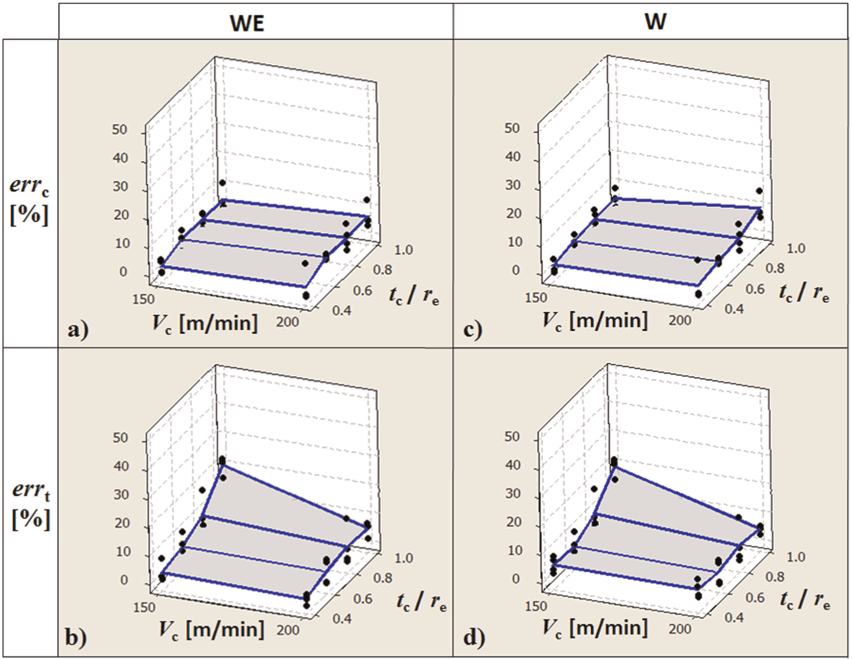
Percentage errors for the star (
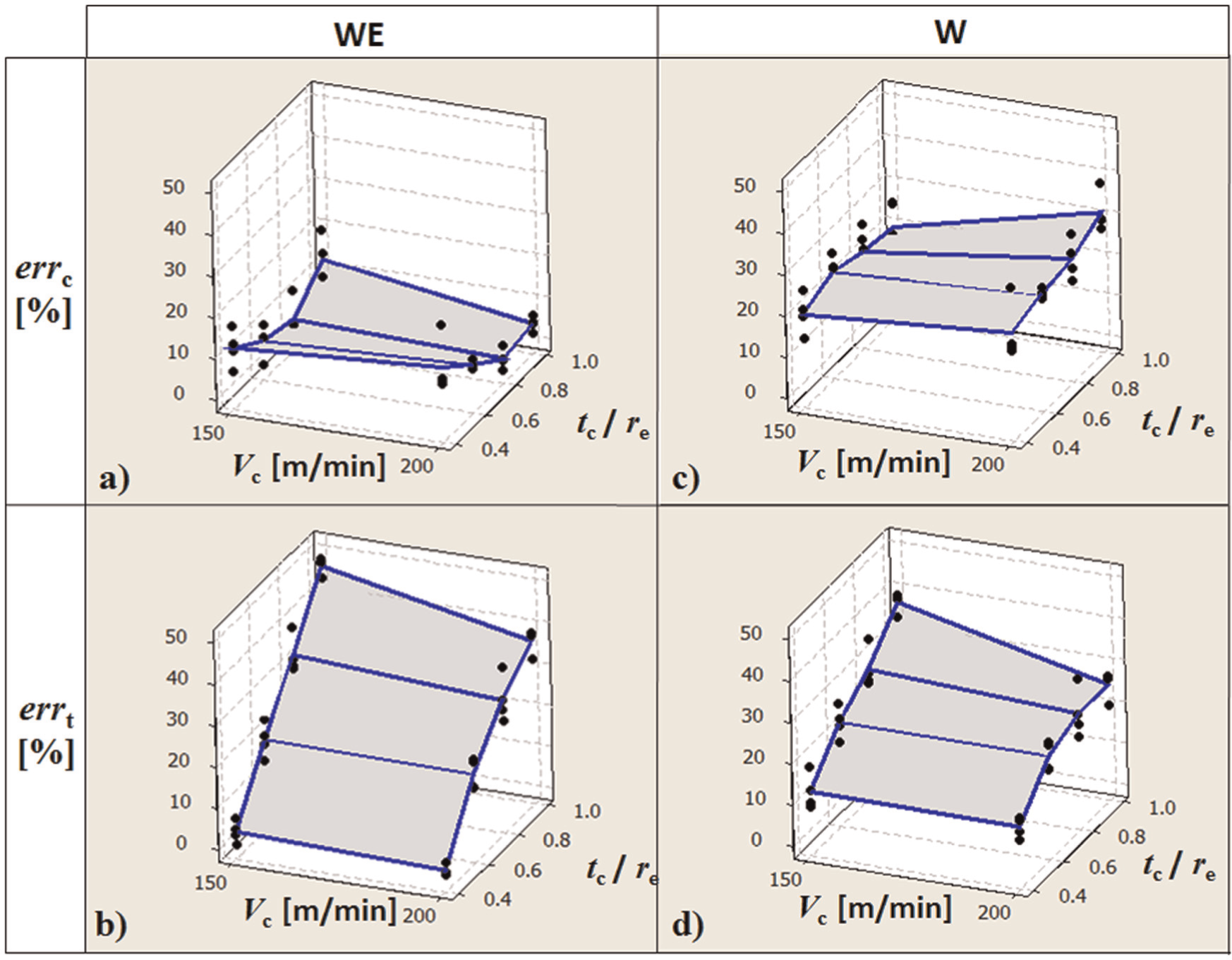
Percentage errors for the diamond (♦) calibration set: (a) errc _WE, (b) errt _WE, (c) errc _W and (d) errt _W.
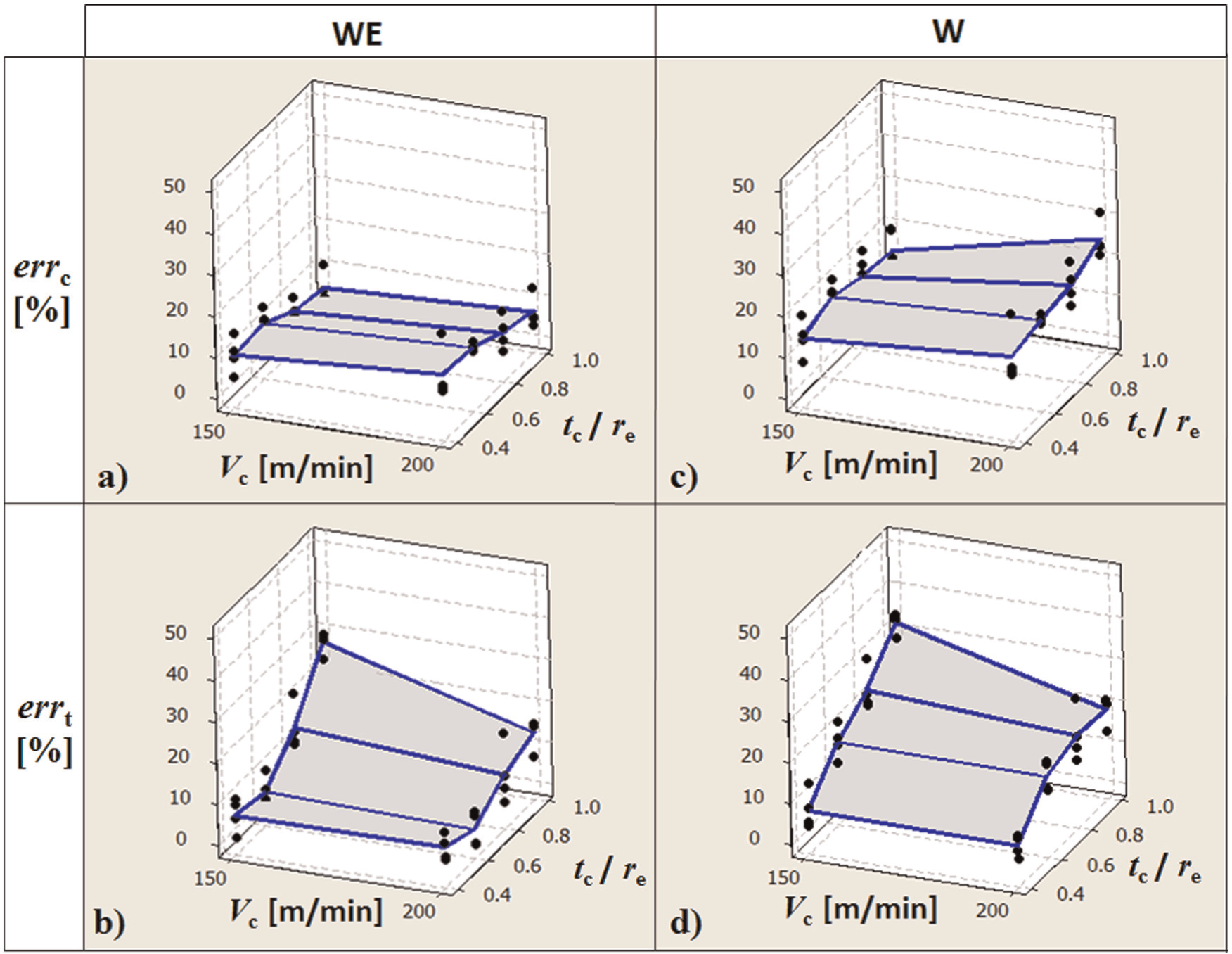
Percentage errors for the square (▪) calibration set: (a) errc _WE, (b) errt _WE, (c) errc _W and (d) errt _W.
The strength of the proposed WE approach is that the model, once calibrated with the best condition (
Model validation
The model prediction performance has been validated by means of the validation design experiments (red dotted box in Figure 17). All the experimental conditions in this set have a different cutting speed than those in the calibration design (blue solid box in Figure 17) in order to prove the model robustness to the cutting speed effects; in fact, the cutting speed is not a model input parameter. The cutting speed for the validation design experiments has been set to 250 m/min to maintain a constant difference among the cutting speed levels. Moreover, when machining in the microscale, it is difficult to reach higher cutting speeds due to the limitations on maximum spindle speeds.
Validation with the best calibration set (
Both the W and the WE model, calibrated with the best calibration set (
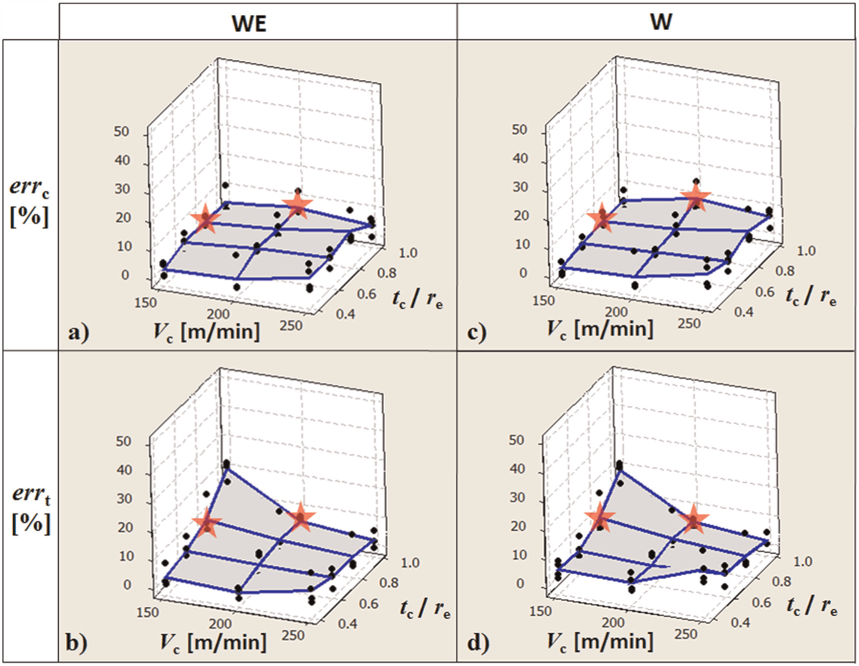
Percentage errors for the star (
Figure 18 shows how the WE model prediction performance is better than the W model prediction performance in the calibration design space and is good also for the experimental conditions of the validation design. This fact highlights how the WE model, once correctly calibrated, is able to accurately predict the cutting forces outside the calibration window. Moreover, the model validation with a cutting speed outside the calibration set proves its robustness to cutting speed effects. In fact, the cutting speed is not a model input parameter, but it is known that the cutting speed affects the material properties (e.g. a cutting speed increase causes a softening effect). For the sake of completeness, Figure 19 shows the cutting and thrust force values that have been measured for all the cutting trials in the experimental database (Table 1) and the values that have been predicted applying the WE approach in the case of the best calibration set (⋆).
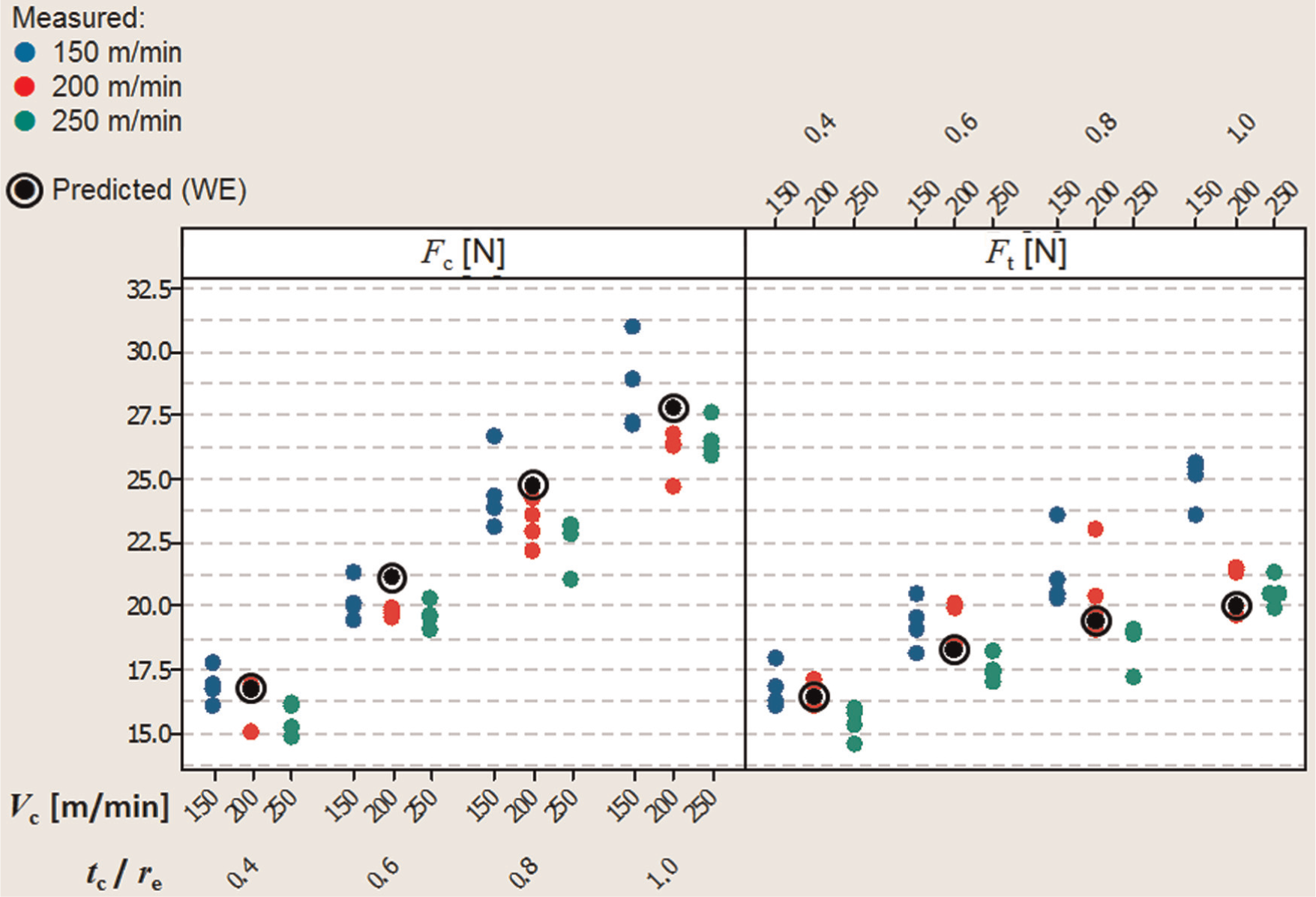
Measured and predicted (WE approach) values of cutting and thrust forces for the star (
Conclusion and future developments
This article has been focused on the Waldorf’s slip-line field model9,10 applied to typical microcutting parameters in both its original version and a modified version implementing the effective rake angle. 4 The purpose has been to demonstrate the model adequacy to predict forces in the microfield. In order to achieve this goal, a clear, modular, objective and repeatable procedure making the selected slip-line field model an applicable and sustainable force prediction instrument in the microscale has been developed.
The model modified version is generally better for the tested calibration conditions but, in particular, at low uncut chip thickness where the model seems to work satisfactorily in the microfield. Such an objective conclusion and the carried out calibration and prediction procedures are important for future developments. Next studies will aim at substituting some procedure modules (Figure 8) to extend the calculation validity overcoming some restrictive assumptions, for example, in the case of the flow stress k calculation (box 5).
Further studies will deal with other target materials and other tool geometries in order to objectively check the model possible extensions. A structured quantitative criterion will be obtained for the calibration condition selection. Moreover, further validation tests for other experimental conditions outside the original experimental design will be carried out in order to extend this article’s results. The model will also be applied to predict shear and ploughing forces, and a suitable validation, based on chip formation micrographs, will be carried out for this purpose.
Footnotes
Appendix 1
Declaration of conflicting interests
The authors declare that there is no conflict of interest.
Funding
This study was partly funded by Regione Lombardia within the project “REMS: Rete Lombarda di Eccellenza per la Meccanica Strumentale e Laboratorio Esteso/Excellence Network for Instrumental Mechanics and Extended Laboratory” (Fondo per la promozione di Accordi Istituzionali, D. Reg. no. 4779 del 14/5/2009).