Sage Journals: Discover world-class research

Abstract

The supplier selection is a key component of the supply chain management. Existing methods for the supplier selection are based on analytic network process. They can handle the interdependence of decision attributes; however, these methods could not guarantee an optimal solution when given vague or incomplete input data. To deal with the uncertainties of input data, we propose methods combining analytic network process with Dempster–Shafer evidence theory. We demonstrate efficiency and accuracy of the proposed method in a numerical example. We demonstrate that the proposed method is flexible and effective in dealing with the supplier selection problem.

Keywords

Supplier selection analytical network process Dempster–Shafer evidence theory Dempster–Shafer/analytic network process

Introduction

The supplier selection plays an important role in the manufacturing process. The companies have to work with different suppliers to carry out their activities so that the components and parts can be delivered on time. The supplier selection is a multi-criteria decision-making (MCDM) problem. A number of MCDM methods have been proposed,^1,2 including analytic hierarchy process (AHP),^3,4 analytic network process (ANP),⁵ technique for order of preference by similarity to ideal solution (TOPSIS)^6,7 and others.⁸ The AHP is a structured technique for organizing and analyzing complex decisions, developed by Saaty^9,10 in the 1970s. It focuses on comparing and evaluating different criteria toward the objective through constructing the hierarchical levels. The AHP does not perform well in situations when there are interactions and dependencies across the criteria at different levels.¹¹ The ANP¹² can overcome the limitations of AHP: it can deal quantitatively with the dependencies and interactions across the elements at various levels. To date, the ANP is the most common tool for tackling the selection problems.^13,14

In the process of determining the optimal supplier, experts’ knowledge plays an important role. For example, in AHP, the comparison matrices are provided by many experts according to their knowledge. Based on experts’ evaluation, we are able to allocate the appropriate weight for the corresponding criteria. However, in many cases, uncertainties emerge in experts’ subjective and quantitative assessment. Moreover, in many situations, it is difficult for us to use a precise way to measure the performance of each decision alternative, especially when dealing with large systems. From this point of view, it is inevitable for us to handle the incomplete or vague information involved in many systems.

Many researchers attempted to solve the supplier selection problem under uncertain environment.^15–18 Several techniques are proposed including fuzzy set and probability-based approaches. Among them, Dempster–Shafer (DS) theory is the most efficient tool capable for handling vague information.^19,20 It is more general than probability and possibility theories and can be applied under uncertain situations even if limited or conflicting information is provided by experts. The basic operations of DS theory allow the users to combine the random and epistemic uncertainties in a more straightforward way without any assumptions. With the ability of coping with the uncertainty or imprecision embedded in evidence, DS theory is widely used in many applications, such as information fusion,^21–23 target recognition^24,25 and decision-making.^26–30

We combine ANP and DS theory in a novel method named DS\ANP. Our method inherits advantages of the flexibility offered by DS theory for the incomplete and vague information and the modeling power of ANP. To the best of our knowledge, this is the first attempt to hybridize the ANP method with DS theory of evidence to solve the supplier selection problems.

This article is structured as follows. The literature review is provided in section “Literature review.” Section “Proposed method” details the proposed method. In section “Proposed method,” our methods are applied to a real-world case. The results of the analysis are discussed in section “Case study.” In section “Case study,” we discuss main findings and contributions. Further studies are proposed in section “Conclusion.”

Literature review

According to the current literatures, suppler selection is typically a MCDM problem. To date, various techniques, such as the AHP, ANP, fuzzy set theory, genetic algorithm, mathematical programming and simple multi-attribute rating technique, have been employed to deal with this problem. Most results on the supplier selection problem can be classified into two groups. The first one is mainly focused on the introduction of mathematical or quantitative decision-making approaches. The second one deals with the uncertain information contained in the supplier selection problem.

Due to the flexibility and simplicity of AHP, it has been very popular in the past decades.^11,31–33 For example, Chan³⁴ combined an interactive selection model with AHP to handle the supplier selection process systematically and quantitatively. Yang and Chen³⁵ incorporated gray relational analysis to the AHP methodology to select the best suppliers for cooperation. Bei et al.³⁶ presented an AHP-based model to identify the most preferred supplier in manufacturing supply chain. Chan and Kumar³ combined fuzzy set theory with AHP and presented a fuzzy extended AHP approach using triangular fuzzy numbers to improve the AHP method and to facilitate global supplier selection process. Chan et al.³⁷ and Lee³⁸ gave a brief review on the applications of fuzzy AHP. Shaw et al.³⁹ integrated fuzzy AHP with fuzzy multi-objective linear programming for selecting the appropriate supplier in the supply chain, addressing the carbon emission issue. Recently, Deng et al.⁴⁰ presented a new effective and feasible representation of uncertain information—D numbers, derived from AHP; the approach is proved to be efficient in studies of supplier selection and environmental impact assessment.⁴¹

In recent years, applications of the ANP in supplier selection have increased substantially compared to AHP. Sarkis and Talluri⁴² built an ANP-based supplier selection model by considering a series of factors including operational, tangible and intangible measures. Gencer and Gürpinar investigated ANP’s application in the supplier selection problem and carried out in an electronic firm. Wu et al.⁴³ proposed an integrated multi-objective decision-making process by using ANP and mixed integer programming to determine the selection of supplier. However, they did not take into account the imprecise or vague information involved in the supply chain systems. Vinodh et al.⁴⁴ presented a fuzzy analytic network process (FANP) approach and used it to select the supplier for an Indian electronics switches manufacturing company.

Efficiency of FANP is undermined by needs to rank fuzzy numbers and difficulties in obtaining the consistency in the fuzzy comparison matrices. The problems need to be addressed before it can be implemented directly into real-world applications. Kuo and Lin⁴⁵ combined ANP with data envelopment analysis (DEA) technique to overcome the deficiency of DEA: the users cannot set up criteria weight preferences. DEA technique is not capable of processing imprecise data or information in the process of determining the optimal decision alternative. Recently, Dou et al.⁴⁶ introduced a gray analytical network process–based (gray ANP–based) model to identify green supplier development programs that will effectively improve suppliers’ performance. The ANP-based model is mainly used to predict the performance of an enterprise in the long run, and its ability to handle the epistemic uncertainty might be jeopardized in many situations. In addition to the above, there are also many other approaches and the hybrid methods dealing with this open issues, for example, the mixture of FANP and fuzzy TOPSIS,⁴⁷ the integration of semi-fuzzy support vector domain description and cooperative coevolution (CC)-Rule method⁴⁸ and linear programming.⁴⁹

Since uncertainty is one of the features of real-world applications, many methods have been proposed to deal with this problem,^50–58 such as fuzzy set theory^59–61 and interval theory.^62–64 For example, Amin et al.⁶⁵ integrated the fuzzy logic and triangular fuzzy numbers with SWOT (strength, weakness, opportunity and threat) in the context of supplier selection. Tao et al.⁶⁶ integrated DEA, AHP and TOPSIS with axiomatic fuzzy set (AFS) theory by combining the advantages of each method.

The fuzzy set theory and the interval theory require that a membership function under uncertain environment is constructed in advance. However, it is difficult to determine values of the membership function before making a decision. When dealing with real-world supply chains, it takes a substantial amount of time to conduct many experiments to calculate values of the membership functions. The interval theory and AFS theory bear the same deficiency. This is why these theories are not practical when real-world applications are concerned.

DS evidence theory is a novel tool capable of handling vague information. It has been applied in many fields of science and engineering to describe uncertainty: decision analysis, pattern recognition, risk assessment, supplier selection and others.^19,52,67 For example, Beynon et al.⁶⁸ combined AHP with evidence theory and used it in multi-criteria decision modeling. Since then, DS/AHP has received great attention.^11,69

Although there are abundant literatures about the selection of suitable supplier, to the authors’ knowledge, there were relatively few works which combined DS evidence theory and ANP to deal with this problem. By combing these two theories together, we take advantage of the flexibility offered by DS theory when dealing with incomplete and vague information and the modeling power of ANP.

Proposed method

First of all, we must identify criteria and sub-criteria for implementing the DS/ANP method. AHP is employed to build the initial weights associated with each criterion and sub-criterion. DS/AHP is used to construct the attribute’s basic probability assignment (BPA). By considering the dependencies and interactions across the criteria, we construct the super matrix formulated by the initial weights. Based on ANP, the weight associated with each attribute can be calculated. By using Dempster’s rule of combination, the performance of each supplier can be determined. The flowchart of the proposed method is shown in Figure 1.

Figure 1.

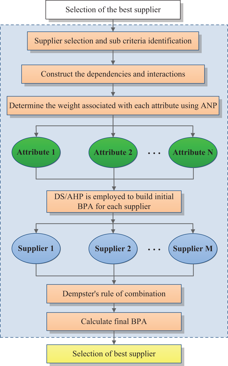
Flowchart of the proposed method.

Supplier selection and sub-criteria identification

To evaluate the performance of each supplier, we must identify all possible elements and factors to be inspected and assessed. We adopt the hierarchical structure for supplier selection, Figure 2, from Vinodh et al.⁴⁴ As can be seen in Figure 2, we have identified five criteria as the dimensions in the ANP model. These are business improvement (BI), extent of fitness (EOF), quality (Q), service (S) and risks (R). The second level consists of various attributes under different criteria. BI has four attributes: reputation of industry (ROI), financial strength (FS), managing ability (MA) and organization customers (OS). EOF has three attributes: sharing of expertise (SOE), flexible practices (FP), and diversified customers (DC). Q has three attributes: low defect rate (LDR), commitment to quality (CTQ) and improved process capacity (IPC). S also has three attributes: on-time delivery (OTD), quick responsiveness (QR) and supplier capacity (SC1). R has three attributes: supply constraint (SC2), buyer–supplier constraint (BSC) and supplier profile (SP). All the attributes and hierarchical structures are adopted from Vinodh et al.⁴⁴

Figure 2.

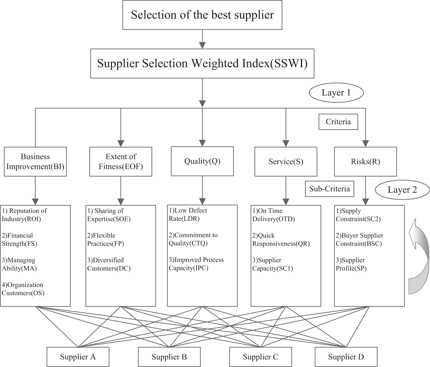
The hierarchical structure for the supplier selection.

In contrast to Vinodh et al.,⁴⁴ we consider the interactions at the second level. A looped arc is used in the ANP model to show such interdependencies (see Figure 2). The alternatives that the decision-maker wishes to evaluate are shown at the bottom of the model. In this article, we take into consideration four decision alternatives: Supplier A, Supplier B, Supplier C and Supplier D.

Constructing the weight associated with each criterion and sub-criterion

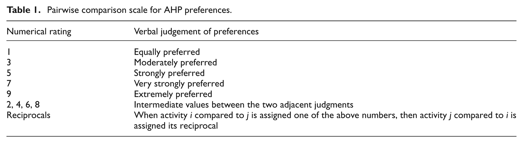
In this step, both AHP and ANP are used to construct the weights across the criteria. For the attributes in Layer 1, AHP¹⁰ is employed to construct such weights. We build a series of pairwise comparisons to establish the relative importance of determinants in achieving the objectives. A ratio of scale 1–9 is used to compare any two criteria. Table 1 displays the pairwise comparison scale for AHP preferences. A score 1 means that these two elements are important equally, while a score of 9 denotes the overwhelming dominance of the element over the comparison element. If an attribute has weaker impact when compared with its comparison element, the range of the scores will be reversed from 1 to 1/9. In addition to this, an index called consistency ratio is built to check the consistency of the weights across all the criteria. These criteria are used to calculate the final supplier selection weighted index (SSWI).

Table 1.

Pairwise comparison scale for AHP preferences.

Numerical rating	Verbal judgement of preferences
1	Equally preferred
3	Moderately preferred
5	Strongly preferred
7	Very strongly preferred
9	Extremely preferred
2, 4, 6, 8	Intermediate values between the two adjacent judgments
Reciprocals	When activity i compared to j is assigned one of the above numbers, then activity j compared to i is assigned its reciprocal

For the criteria in Layer 2, there are interdependencies among these criteria. Here, ANP is employed to calculate the weight of each sub-criterion. The pairwise comparisons are made to capture interdependencies among the sub-criteria. One such comparison is presented in Table 2. It gives the result of BI with ROI as the controlling attribute over other sub-criteria. As shown in Table 2, the ROI is the criterion important equally to FS, MA and OS.

Table 2.

Pairwise comparison matrix for the sub-criteria in Layer 2 under the ROI criteria.

ROI	FS	MA	OS	Weight
FS	1	3	7	0.6694
MA	1/3	1	3	0.2426
OS	1/7	1/3	1	0.0879

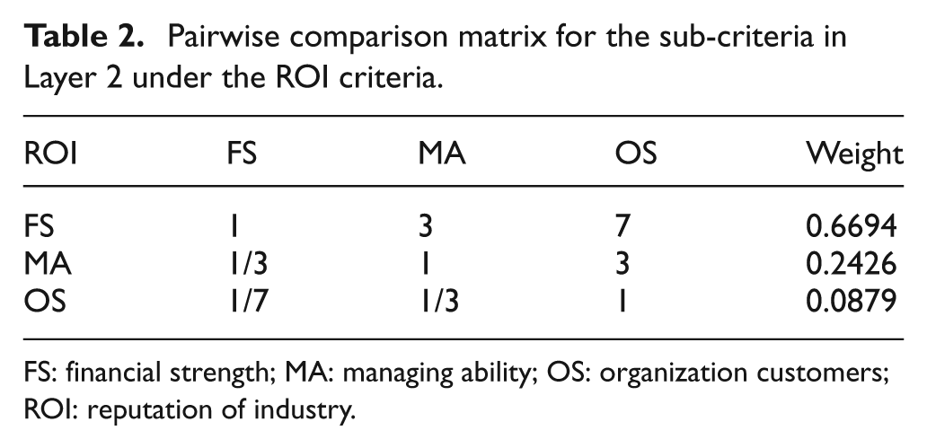
FS: financial strength; MA: managing ability; OS: organization customers; ROI: reputation of industry.

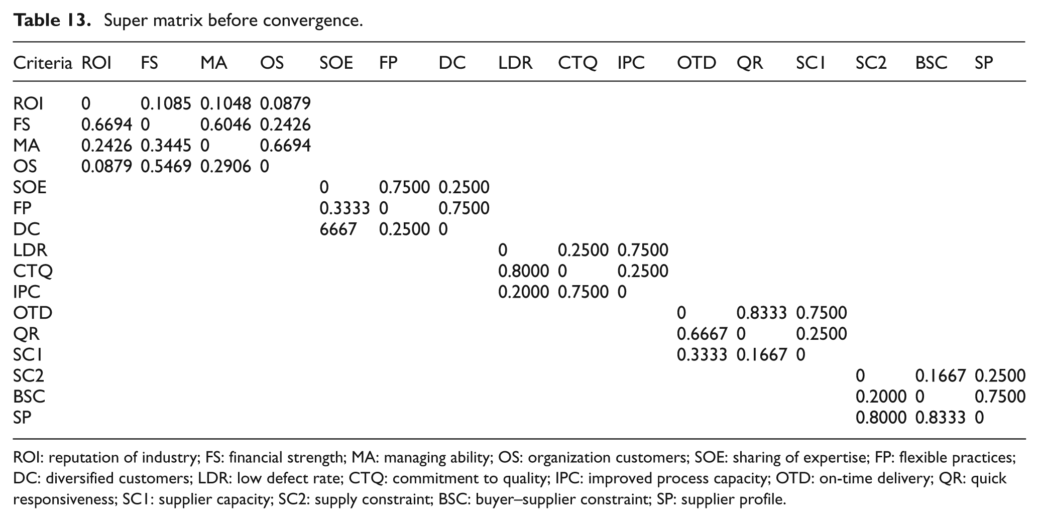
As can be seen from Table 2, FS has the maximum impact (0.6694) on the criteria BI over other attributes when ROI is treated as the controlling attribute. In a similar way, the other pairwise comparison matrices can be built. In ANP, the super matrix is formulated by such kind of pairwise comparison matrices, which allows us for the resolution of interdependencies across all the attributes. After the super matrix converges to a stable state, the relative importance measures for each attribute can be obtained. Different from traditional DS/AHP, we take into consideration the interactions and interdependencies existing in the supplier selection problem. DS/ANP is a generalization of DS/AHP, and it makes DS/AHP more flexible and more reasonable when dealing with the complex systems.

Building BPA associated with each criterion

In this step, DS/AHP is used to construct the BPA associated with each decision alternative. DS/AHP is proposed by Beynon et al.,⁶⁸ which enables a measure of uncertainty and ignorance to be constructed. In DS/AHP, the decision-makers express their preference by comparing a group of decision alternatives to θ, while in AHP, by making pairwise comparisons between individual decision alternatives. For DS/AHP, the 5-unit scale is adopted as a basis for discriminating levels of knowledge.⁷⁰ Normally, p in this scale has the value of 0.2159.

Here, we give a brief introduction to the DS/AHP approach. For the ROI attribute, we build the following knowledge matrix as shown in Table 3. The values in the final column are the measures of groups of decision alternatives in each row with respect to θ. It can be noted that A, D viewed as extremely favorable when compared to θ.

Table 3.

Initial knowledge matrix for ROI criterion.

ROI	{A, D}	{C}	θ
{A, D}	1	0	6p
{C}	0	1	4p
θ	1/(6p)	1/(4p)	1

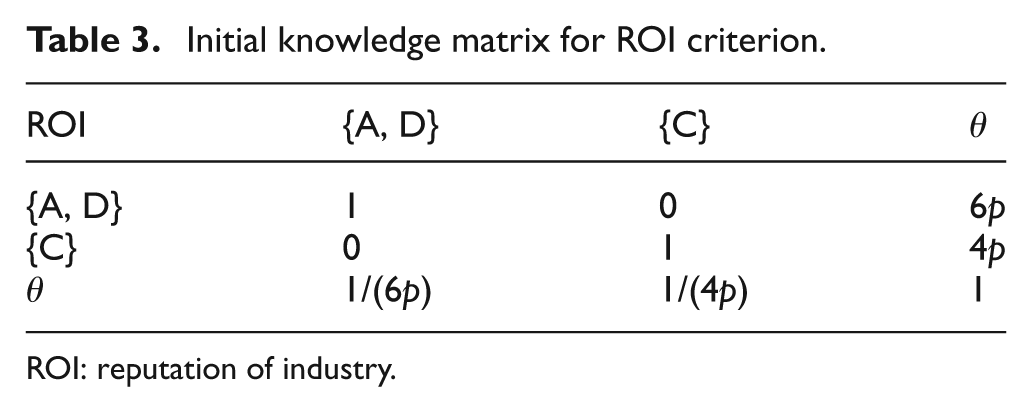
ROI: reputation of industry.

Following the method in Anderson,⁷¹ we can construct the weights derived as the eigenvectors of the knowledge matrix, which are shown in Table 4. We treat these priority allocations as BPA. As a consequence, we have

m_{1} ({A, D}) = 0.3625, m ({D}) = 0.2417, m ({θ}) = 0.3958

Table 4.

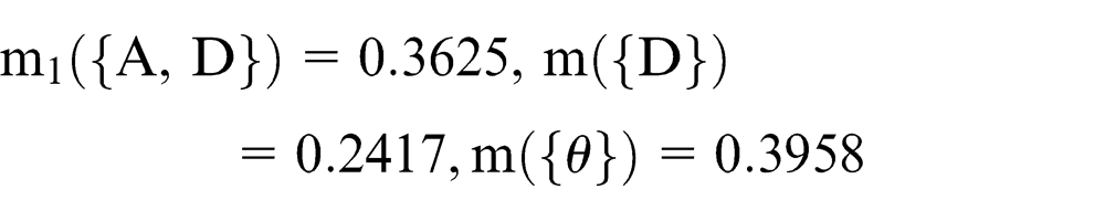
Priority values for groups of decision alternatives and θ.

ROI	Priority
A, D	0.7153
C	0.1870
θ	0.0977

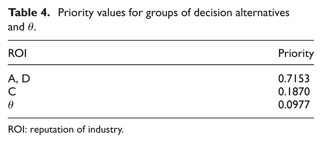
ROI: reputation of industry.

In the same way, we can construct the BPA for the other criteria. And thus, all the BPAs can be built.

Ranking all the suppliers

In the second step, by using ANP, we have calculated the weight for each attribute in Layer 2. In addition, the BPA associated with every criterion has been built. However, we do not combine them all together right now. At this step, we combine the weight and the BPA of every attribute.

Definition 3.1

Let U be the frame of discernment and $m_{j}^{d}$ be the new BPA after discounting. The discounting operation is accomplished as follows

m_{j}^{d} (A_{j}) = {\begin{matrix} α_{j} m_{j} (A_{j}), A_{j} \neq U \\ 1 - α_{j} + α_{j} m_{j} (U), A_{j} = U \end{matrix}

(1)

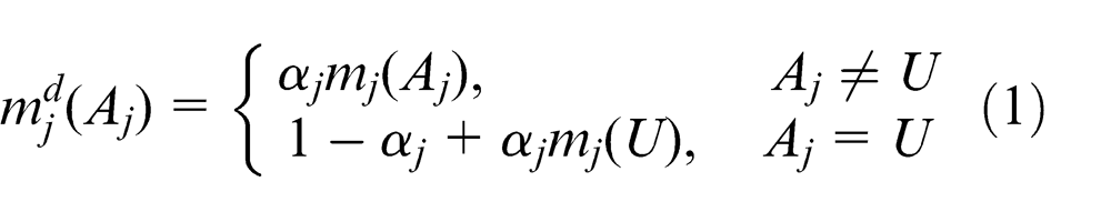
where m_j is the BPA of focal element A_j.

By making full use the discount technique shown in Definition 3.1, we will apply the weight of each criterion into the corresponding BPA. According to Dempster’s rule of combination, the BPA associated with every attribute can be aggregated. In this way, the performance of each decision alternative can be calculated.

Case study

The case study has been implemented at Salzer Electronics Limited (hereafter referred to Salzer).⁴⁴ Salzer is a manufacturing company producing Cam operated rotary switches and a series of other products, which was founded in 1984. As shown in Figure 2, the best supplier can be determined based on the calculation of SSWI. SSWI is associated with five factors: BI, EOF, Q, S and R.

First of all, we construct the knowledge matrix for each criterion. Figure 3 shows the DS/AHP decision tree used to determine the supplier. For instance, for the attribute ROI, from Figure 3, it can be noticed that two distinct groups of decision alternatives ({A, D} and {C}) have been identified as being comparable with the frame of discernment Θ. Knowledge matrices of other criteria can be built in a similar way. Table 5 shows us the initial knowledge matrix for every attribute.

Figure 3.

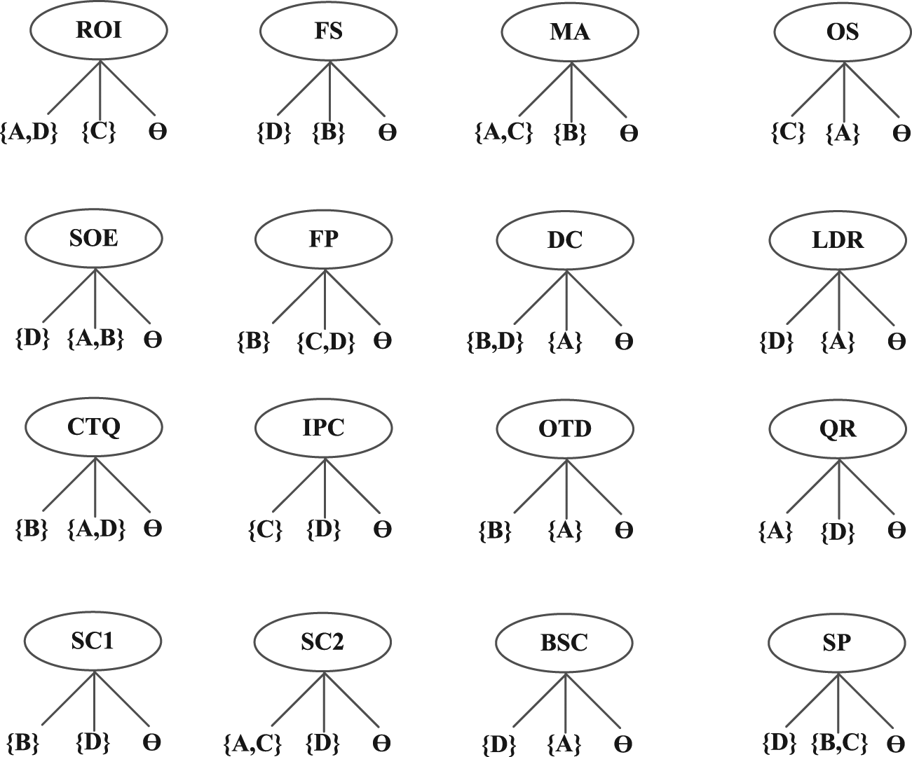
Decisions when only single criterion is considered.

Table 5.

Initial knowledge matrix for each attribute.

ROI	{A, D}	{C}	θ	SOE	{D}	{A, B}	θ	CTQ	{B}	{A, D}	θ	SC1	{B}	{D}	θ
{A, D}	1	0	6 p	{D}	1	0	6 p	{B}	1	0	6 p	{B}	1	0	6 p
{C}	0	1	4 p	{A, B}	0	1	5 p	{A, D}	0	1	2 p	{D}	0	1	2 p
θ	1/(6p)	1/(4p)	1	θ	1/(6p)	1/(5p)	1	θ	1/(6p)	1/(2p)	1	θ	1/(6p)	1/(2p)	1
FS	{D}	{B}	θ	FP	{B}	{C, D}	θ	IPC	{C}	{D}	θ	SC2	{A, C}	{D}	θ
{D}	1	0	4p	{B}	1	0	5p	{C}	1	0	4p	{A, C}	1	0	5p
{B}	0	1	3p	{C, D}	0	1	4p	{D}	0	1	2p	{D}	0	1	4p
θ	1/(4p)	1/(3p)	1	θ	1/(5p)	1/(4p)	1	θ	1/(4p)	1/(2p)	1	θ	1/(5p)	1/(4p)	1
MA	{A, C}	{B}	θ	DC	{B, D}	{A}	θ	OTD	{B}	{A}	θ	BSC	{D}	{A}	θ
{A, C}	1	0	6p	{B, D}	1	0	5p	{B}	1	0	5p	{D}	1	0	6p
{B}	0	1	2p	{A}	0	1	3p	{A}	0	1	3p	{A}	0	1	3p
θ	1/(6p)	1/(2p)	1	θ	1/(5p)	1/(3p)	1	θ	1/(5p)	1/(3p)	1	θ	1/(6p)	1/(3p)	1
OS	{C}	{A}	θ	LDR	{D}	{A}	θ	QR	{A}	{D}	θ	SP	{D}	{B, C}	θ
{C}	1	0	4p	{D}	1	0	6p	{A}	1	0	3p	{D}	1	0	5p
{A}	0	1	2p	{A}	0	1	2p	{D}	0	1	2p	{B, C}	0	1	4p
θ	1/(4p)	1/(2p)	1	θ	1/(6p)	1/(2p)	1	θ	1/(3p)	1/(2p)	1	θ	1/(5p)	1/(4p)	1

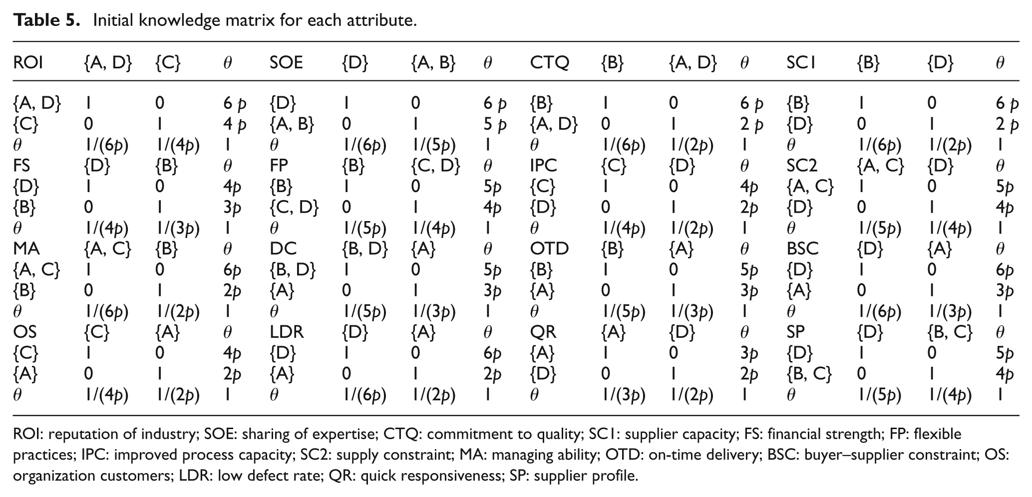
ROI: reputation of industry; SOE: sharing of expertise; CTQ: commitment to quality; SC1: supplier capacity; FS: financial strength; FP: flexible practices; IPC: improved process capacity; SC2: supply constraint; MA: managing ability; OTD: on-time delivery; BSC: buyer–supplier constraint; OS: organization customers; LDR: low defect rate; QR: quick responsiveness; SP: supplier profile.

Based on the data in Table 5, following the approach presented in section “Building BPA associated with each criterion,” we can construct BPA for each attribute shown in Table 6.

Table 6.

The initialized BPA associated with each attribute.

Criteria	BPA
ROI	m {A, D} = 0.3625, m {C} = 0.2417, m {Θ} = 0.3958
FS	m {D} = 0.2952, m {B} = 0.2214, m {Θ} = 0.4834
MA	m {A, C} = 0.4124, m {B} = 0.1375, m {Θ} = 0.4502
OS	m {C} = 0.3187, m {A} = 0.1594, m {Θ} = 0.5219
SOE	m {D} = 0.3419, m {A, B} = 0. 2849, m {Θ} = 0. 3732
FP	m {B} = 0. 3215, m {C, D} = 0. 2572, m {Θ} = 0. 4212
DC	m {B, D} = 0. 3436, m {A} = 0. 2062, m {Θ} = 0. 4502
LDR	m {D} = 0. 4124, m {A} = 0. 1375, m {Θ} = 0. 4502
CTQ	m {B} = 0. 4124, m {A, D} = 0. 1375, m {Θ} = 0. 4502
IPC	m {C} = 0. 3187, m {D} = 0. 1594, m {Θ} = 0. 5219
OTD	m {B} = 0. 3436, m {A} = 0. 2062, m {Θ} = 0. 4502
QR	m {A} = 0. 2597, m {D} = 0. 1732, m {Θ} = 0. 5671
SC1	m {B} = 0. 4124, m {D} = 0. 1375, m {Θ} = 0. 4502
SC2	m {A, C} = 0. 3215, m {D} = 0. 2572, m {Θ} = 0. 4212
BSC	m {D} = 0. 3858, m {A} = 0. 1929, m {Θ} = 0. 4212
SP	m {D} = 0. 3215, m {B, C} = 0. 2572, m {Θ} = 0. 4212

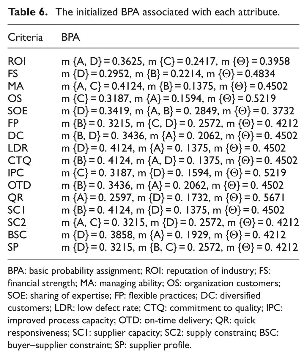
BPA: basic probability assignment; ROI: reputation of industry; FS: financial strength; MA: managing ability; OS: organization customers; SOE: sharing of expertise; FP: flexible practices; DC: diversified customers; LDR: low defect rate; CTQ: commitment to quality; IPC: improved process capacity; OTD: on-time delivery; QR: quick responsiveness; SC1: supplier capacity; SC2: supply constraint; BSC: buyer–supplier constraint; SP: supplier profile.

In what follows, the weight of every sub-criterion in Layer 2 is determined using ANP. In ANP, AHP is used to evaluate each criterion’s weight, which is introduced in detail in section “Constructing the weight associated with each criterion and sub-criterion.”Table 7 shows the judgment matrix of each criterion in Layer 2.

Table 7.

Pairwise comparison matrix for the sub-criteria in Layer 2 under different controlling criteria.

ROI	FS	MA	OS	Weight	SOE	FP	DC	Weight	IPC	LDR	CTQ	Weight
FS	1	3	7	0.6694	FP	1	1/2	0.3333	LDR	1	3	0.7500
MA	1/3	1	3	0.2426	DC	2	1	0.6667	CTQ	1/3	1	0.2500
OS	1/7	1/3	1	0.0879	FP	SOE	DC	Weight	OTD	QR	SC1	Weight
FS	ROI	MA	OS	Weight	SOE	1	3	0.7500	QR	1	2	0.6667
ROI	1	1/4	1/4	0.1085	DC	1/3	1	0.2500	SC1	1/2	1	0.3333
MA	4	1	1/2	0.3445	DC	SOE	FP	Weight	QR	OTD	SC1	Weight
OS	4	2	1	0.5469	SOE	1	1/3	0.2500	OTD	1	5	0.8333
MA	ROI	FS	OS	Weight	FP	3	1	0.7500	SC1	1/5	1	0.1667
ROI	1	1/4	1/4	0.1048	LDR	CTQ	IPC	Weight	SC1	OTD	QR	Weight
FS	4	1	3	0.6046	CTQ	1	4	0.8000	OTD	1	3	0.7500
OS	4	1/3	1	0.2906	IPC	1/4	1	0.2000	QR	1/3	1	0.2500
OS	ROI	MA	FS	Weight	CTQ	LDR	IPC	Weight	SC2	BSC	SP	Weight
ROI	1	1/3	1/7	0.0879	LDR	1	1/3	0.2500	BSC	1	1/4	0.2000
MA	3	1	1/3	0.2426	IPC	3	1	0.7500	SP	4	1	0.8000
FS	7	3	1	0.6694	SP	SC2	BSC	Weight
BSC	SC2	SP		Weight	SC2	1	1/3	0.2500
SC2	1	1/5		0.1667	BSC	3	1	0.7500
SP	5	1		0.8333

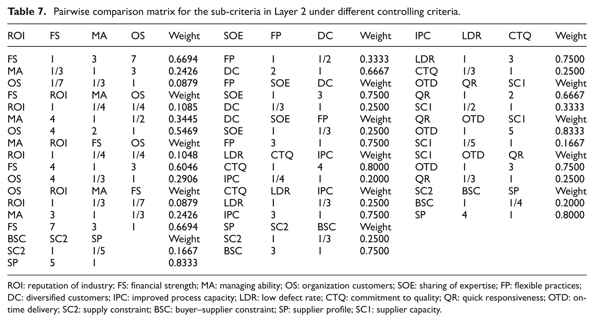
ROI: reputation of industry; FS: financial strength; MA: managing ability; OS: organization customers; SOE: sharing of expertise; FP: flexible practices; DC: diversified customers; IPC: improved process capacity; LDR: low defect rate; CTQ: commitment to quality; QR: quick responsiveness; OTD: on-time delivery; SC2: supply constraint; BSC: buyer–supplier constraint; SP: supplier profile; SC1: supplier capacity.

Next, the relative importance of each dimension for a determinant is obtained through a pairwise comparison matrix. Four such matrices can be formulated in the present case. The matrices for the criteria BI, EOF, Q, S and R are shown in Tables 8 –10. As for the criteria in the first layer, their weights are shown in Table 11.

Table 8.

Pairwise comparisons for attributes BI and EOF.

Pairwise comparisons for BI attribute
BI	ROI	FS	MA	OS	Weight
ROI	1	2	5	3	0.0882
FS	1/2	1	3	2	0.1570
MA	1/5	1/3	1	1/2	0.4829
OS	1/3	1/2	2	1	0.2720
Pairwise comparisons for EOF criteria
EOF	SOE	FP	DC	Weight
SOE	1	3	2	0.5472
FP	1/3	1	2	0.2631
DC	1/2	1/2	1	0.1897

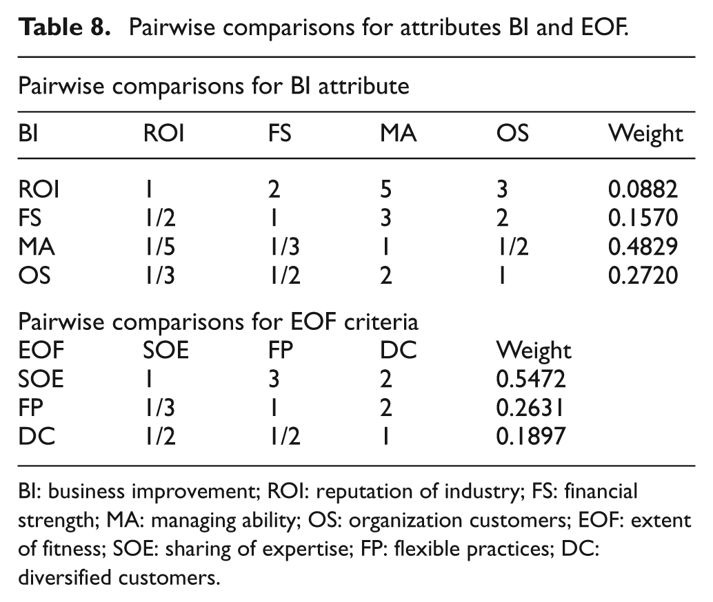
BI: business improvement; ROI: reputation of industry; FS: financial strength; MA: managing ability; OS: organization customers; EOF: extent of fitness; SOE: sharing of expertise; FP: flexible practices; DC: diversified customers.

Table 9.

Pairwise comparisons for attributes Q and S

Pairwise comparisons for Q attribute
Quality	LDR	CTQ	IPC	Weight
LDR	1	1/3	1/2	0.1634
CTQ	3	1	2	0.5396
IPC	2	1/2	1	0.2970
Pairwise comparisons for S criteria
Services	OTD	QR	SC	Weight
OTD	1	3	7	0.6694
QR	1/3	1	3	0.2426
SC	1/7	1/3	1	0.1897

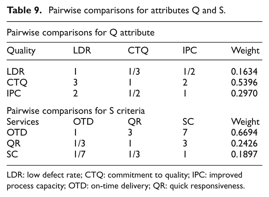
LDR: low defect rate; CTQ: commitment to quality; IPC: improved process capacity; OTD: on-time delivery; QR: quick responsiveness.

Table 10.

Pairwise comparisons for Risks (R) criteria.

Risks	SC	BSC	SP	Weight
SC	1	1/2	1/3	0.1634
BSC	2	1	1/2	0.2970
SP	3	2	1	0.5396

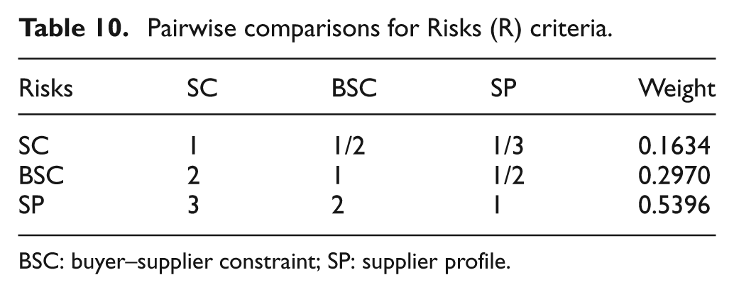
BSC: buyer–supplier constraint; SP: supplier profile.

Table 11.

Weight of each criterion in Layer 1 (CI = 0.0895).

	BI	EOF	Q	S	R	Eigen vector
BI	1	1/2	1/4	1/5	3	0.1089
EOF	2	1	1/2	1/3	2	0.1491
Q	4	2	1	1/2	2	0.2538
S	5	3	2	1	3	0.4028
R	1/3	1/2	1/2	1/3	1	0.0854

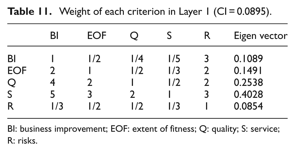
BI: business improvement; EOF: extent of fitness; Q: quality; S: service; R: risks.

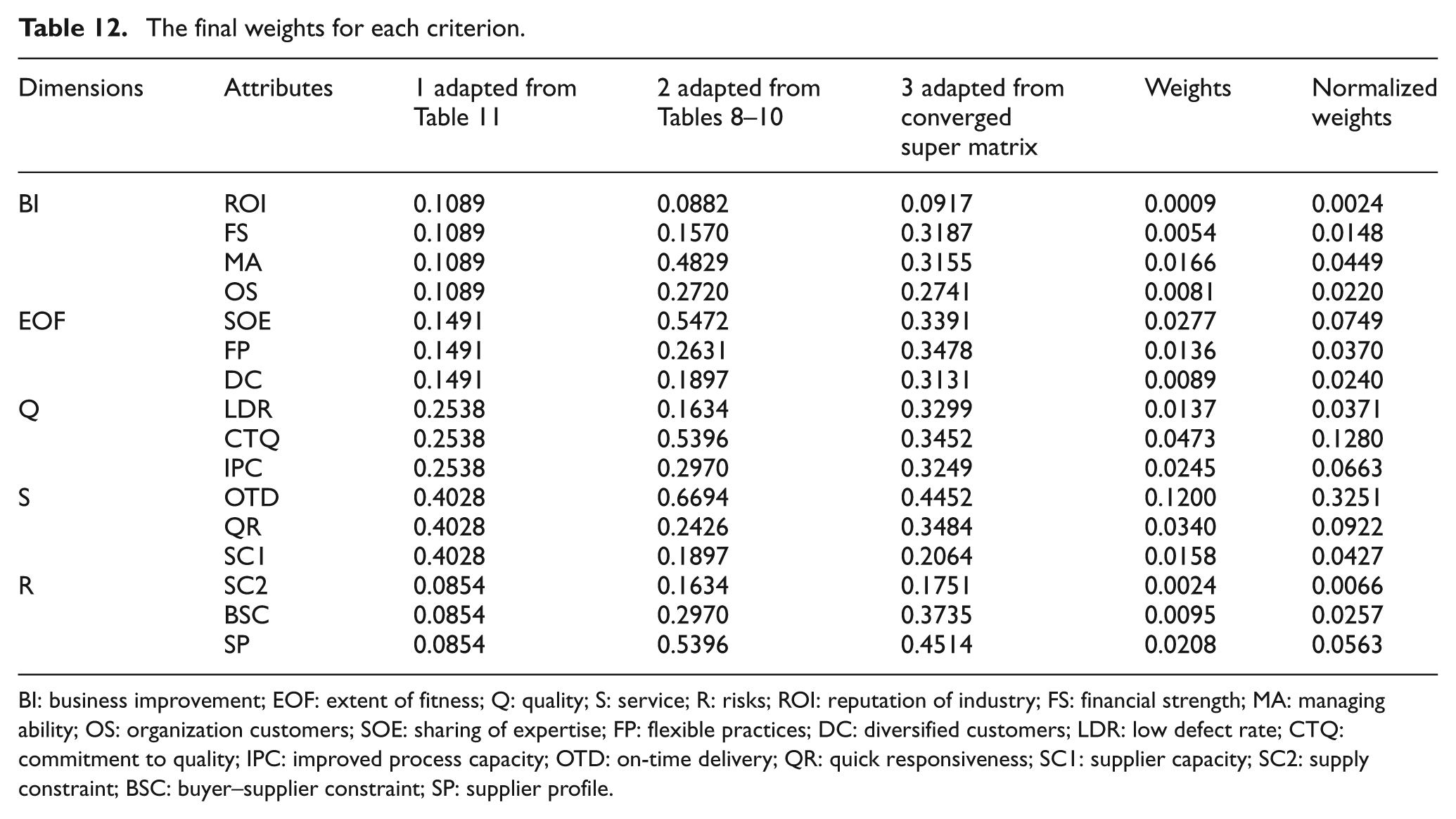
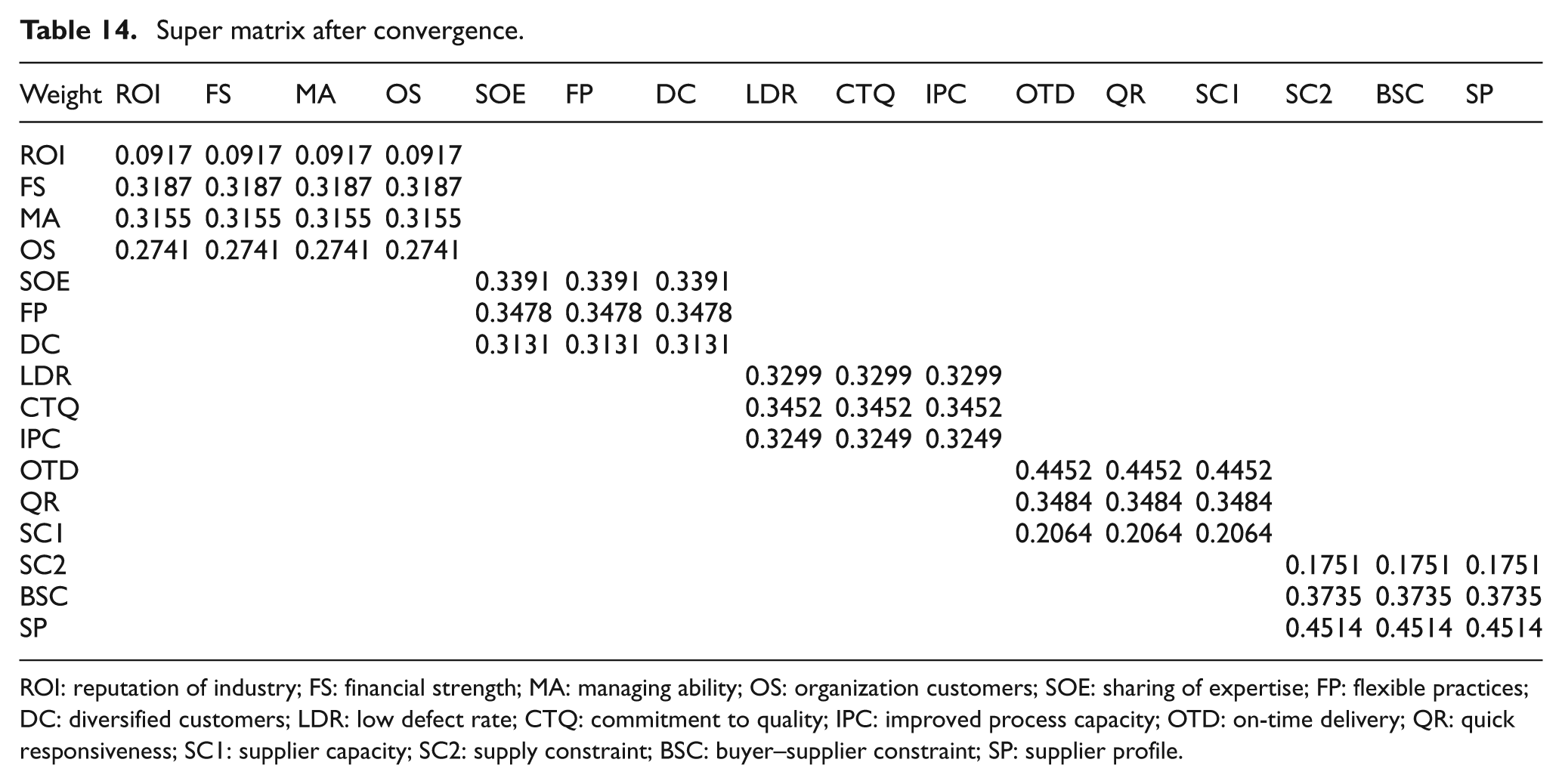
In what follows, the weights for each attribute can be built. The third column in Table 12 shows the weight associated with the criteria in the first layer, while the fourth column displays the relative importance of the attributes in the second layer. The data in the fifth column is adopted from the converged super matrix as shown in Tables 13 and 14. We obtain the weight associated with each attribute in the sixth column. For example, for the attribute FS, its final weight is calculated as follows

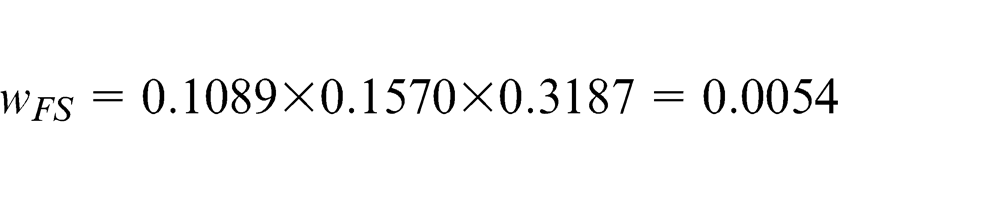
w_{FS} = 0.1089 \times 0.1570 \times 0.3187 = 0.0054

Table 12.

The final weights for each criterion.

Dimensions	Attributes	1 adapted from Table 11	2 adapted from Tables 8 –10	3 adapted from converged super matrix	Weights	Normalized weights
BI	ROI	0.1089	0.0882	0.0917	0.0009	0.0024
	FS	0.1089	0.1570	0.3187	0.0054	0.0148
	MA	0.1089	0.4829	0.3155	0.0166	0.0449
	OS	0.1089	0.2720	0.2741	0.0081	0.0220
EOF	SOE	0.1491	0.5472	0.3391	0.0277	0.0749
	FP	0.1491	0.2631	0.3478	0.0136	0.0370
	DC	0.1491	0.1897	0.3131	0.0089	0.0240
Q	LDR	0.2538	0.1634	0.3299	0.0137	0.0371
	CTQ	0.2538	0.5396	0.3452	0.0473	0.1280
	IPC	0.2538	0.2970	0.3249	0.0245	0.0663
S	OTD	0.4028	0.6694	0.4452	0.1200	0.3251
	QR	0.4028	0.2426	0.3484	0.0340	0.0922
	SC1	0.4028	0.1897	0.2064	0.0158	0.0427
R	SC2	0.0854	0.1634	0.1751	0.0024	0.0066
	BSC	0.0854	0.2970	0.3735	0.0095	0.0257
	SP	0.0854	0.5396	0.4514	0.0208	0.0563

BI: business improvement; EOF: extent of fitness; Q: quality; S: service; R: risks; ROI: reputation of industry; FS: financial strength; MA: managing ability; OS: organization customers; SOE: sharing of expertise; FP: flexible practices; DC: diversified customers; LDR: low defect rate; CTQ: commitment to quality; IPC: improved process capacity; OTD: on-time delivery; QR: quick responsiveness; SC1: supplier capacity; SC2: supply constraint; BSC: buyer–supplier constraint; SP: supplier profile.

Table 13.

Super matrix before convergence.

Criteria	ROI	FS	MA	OS	SOE	FP	DC	LDR	CTQ	IPC	OTD	QR	SC1	SC2	BSC	SP
ROI	0	0.1085	0.1048	0.0879
FS	0.6694	0	0.6046	0.2426
MA	0.2426	0.3445	0	0.6694
OS	0.0879	0.5469	0.2906	0
SOE					0	0.7500	0.2500
FP					0.3333	0	0.7500
DC					6667	0.2500	0
LDR								0	0.2500	0.7500
CTQ								0.8000	0	0.2500
IPC								0.2000	0.7500	0
OTD											0	0.8333	0.7500
QR											0.6667	0	0.2500
SC1											0.3333	0.1667	0
SC2														0	0.1667	0.2500
BSC														0.2000	0	0.7500
SP														0.8000	0.8333	0

ROI: reputation of industry; FS: financial strength; MA: managing ability; OS: organization customers; SOE: sharing of expertise; FP: flexible practices; DC: diversified customers; LDR: low defect rate; CTQ: commitment to quality; IPC: improved process capacity; OTD: on-time delivery; QR: quick responsiveness; SC1: supplier capacity; SC2: supply constraint; BSC: buyer–supplier constraint; SP: supplier profile.

Table 14.

Super matrix after convergence.

Weight	ROI	FS	MA	OS	SOE	FP	DC	LDR	CTQ	IPC	OTD	QR	SC1	SC2	BSC	SP
ROI	0.0917	0.0917	0.0917	0.0917
FS	0.3187	0.3187	0.3187	0.3187
MA	0.3155	0.3155	0.3155	0.3155
OS	0.2741	0.2741	0.2741	0.2741
SOE					0.3391	0.3391	0.3391
FP					0.3478	0.3478	0.3478
DC					0.3131	0.3131	0.3131
LDR								0.3299	0.3299	0.3299
CTQ								0.3452	0.3452	0.3452
IPC								0.3249	0.3249	0.3249
OTD											0.4452	0.4452	0.4452
QR											0.3484	0.3484	0.3484
SC1											0.2064	0.2064	0.2064
SC2														0.1751	0.1751	0.1751
BSC														0.3735	0.3735	0.3735
SP														0.4514	0.4514	0.4514

ROI: reputation of industry; FS: financial strength; MA: managing ability; OS: organization customers; SOE: sharing of expertise; FP: flexible practices; DC: diversified customers; LDR: low defect rate; CTQ: commitment to quality; IPC: improved process capacity; OTD: on-time delivery; QR: quick responsiveness; SC1: supplier capacity; SC2: supply constraint; BSC: buyer–supplier constraint; SP: supplier profile.

After normalization, the weights are shown in the final column of Table 12. Next, according to the discounting operation shown in equation (1) and Dempster’s combination rule, we can build the performance for each decision alternatives. In order to demonstrate the efficiency of the proposed method, we have compared it with DS/AHP method proposed in Beynon.⁷⁰Table 15 and Figure 4 show us the performance of each supplier. Note that Supplier B has the highest priority weight both in DS/AHP and DS/ANP approaches. In addition to this, there is a 22.55% level of combined uncertainty in the DS/ANP, while there is a 17.48% level of combined uncertainty in DS/AHP. Besides, from Figure 4, we can also find that the interdependencies and interactions across the criteria play a vital role in determining the performance associated with each decision alternatives. For example, for the decision alternative D, its priority weight in DS/ANP approach is less than in DS/AHP method by a degree of 16%.

Table 15.

The comparison results between DS/ANP and DS/AHP.

Decision alternatives	DS\ANP	DS\AHP
{A}	0.1919	0.1878
{B}	0.3715	0.3907
{C}	0.0272	0.0346
{D}	0.1108	0.1325
{A, C}	0.0155	0.0190
{A, D}	0.0162	0.0195
{C, D}	0.0071	0.0071
{B, D}	0.0060	0.0067
{B, C}	0.0112	0.0085
{Θ}	0.2255	0.1748

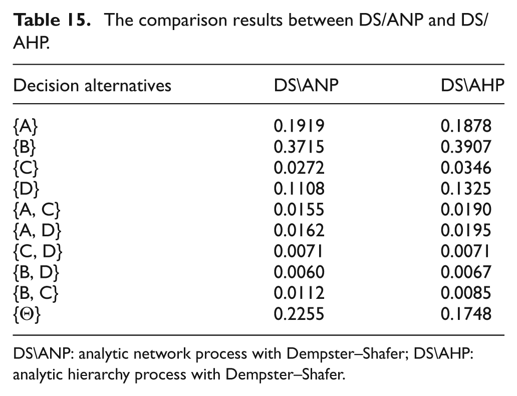
DS\ANP: analytic network process with Dempster–Shafer; DS\AHP: analytic hierarchy process with Dempster–Shafer.

Figure 4.

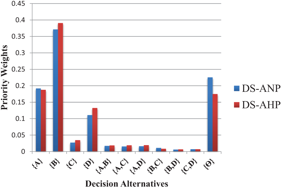
The comparison between DS/ANP and DS/AHP.

Conclusion

An ideal manufacturing requires efficient suppliers. To handle the independencies and the uncertain information on potential suppliers, we proposed a new method DS/ANP based on the ANP method and DS theory of evidence. To the best of our knowledge, this is the first attempt to deal with supplier selection in a manufacturing organization using the hybrid DS/ANP approach. The advantage of the proposed method is that it overcomes the shortcomings of AHP by considering the dependencies and uncertainty across the selection criteria and provides us with a simple and effective way for selecting the supplier. By quantitatively comparing our method with DS/AHP approach, we have shown that the proposed method provides a systematic and optimal tool of decision-making.

The proposed method provides a way for simplified modeling of complex MCDM problems. In addition to this, we can quantify many subjective judgments by taking advantage of the experts’ experience. The decision-making systems are becoming more and more complex nowadays, filled with imprecise and vague information. DS theory is good at capturing such kind of uncertain information, and it provides us with a flexible and effective tool to deal with the supplier selection problem under uncertain environment. Although the model has been verified on a small example, including four distinct decision alternatives and 16 attributes, it is capable for solving more complex problems. In future studies, we will demonstrate on large-scale data sets that the method proposed in this article could help us to reduce the risks of making poor investment decisions when dealing with complex networks of suppliers.

Footnotes

Acknowledgements

The authors are grateful to reviewers for their criticism and constructive comments.

Declaration of Conflicting Interests

The author(s) declared no potential conflicts of interest with respect to the research, authorship, and/or publication of this article.

Funding

The author(s) disclosed receipt of the following financial support for the research, authorship, and/or publication of this article: The work is partially supported by National Natural Science Foundation of China (grant no. 61174022); R&D Program of China (2012BAH07B01); National High Technology Research and Development Program of China (863 Program) (grant no. 2013AA013801); Science and Technology Planning Project of Guangdong Province, China (grant nos 2010B010600034, 2012B091100192); Business Intelligence Key Team of Guangdong University of Foreign Studies (grant no. TD1202) and the open funding project of State Key Laboratory of Virtual Reality Technology and Systems, Beihang University (grant no. BUAA-VR-14KF-02).

References

Alsyouf

Al-Araidah

Tates

. A multi-criteria decision-making framework for assessing the quality and cost of facility layout alternatives: a case study. Proc IMechE, Part B: J Engineering Manufacture 2012; 226(2): 353–364.

Peng

Yeh

Lai

. Similarity-based method for multiresponse optimization problems with intuitionistic fuzzy sets. Proc IMechE, Part B: J Engineering Manufacture 2013; 227(6): 908–916.

Chan

FTS

Kumar

. Global supplier development considering risk factors using fuzzy extended AHP-based approach. Omega 2007; 35(4): 417–431.

Zhang

Deng

Chan

. A modified multi-criterion optimization genetic algorithm for order distribution in collaborative supply chain. Appl Math Model 2013; 37(14): 7855–7864.

Chen

Shih

Shyur

. A business strategy selection of green supply chain management via an analytic network process. Comp Math Appl 2012; 64(8): 2544–2557.

Chakladar

Chakraborty

. A combined TOPSIS-AHP-method-based approach for non-traditional machining processes selection. Proc IMechE, Part B: J Engineering Manufacture 2008; 222(12): 1613–1623.

Shidpour

Shahrokhi

Bernard

. A multi-objective programming approach, integrated into the TOPSIS method, in order to optimize product design; in three-dimensional concurrent engineering. Comput Ind Eng 2013; 63(4): 875–885.

Chen

Zhang

Tian

. An approach to partner selection in virtual enterprises based on grey relational analysis. Proc IMechE, Part B: J Engineering Manufacture 2011; 225(12): 2296–2301.

Saaty

. The analytic hierarchy process. New York: McGraw-Hill, 1980.

10.

Saaty

. How to make a decision: the analytic hierarchy process. Eur J Oper Res 1990; 48(1): 9–26.

11.

Saaty

. The modern science of multicriteria decision making and its practical applications: the AHP/ANP approach. Oper Res 2013; 61(5): 1101–1118.

12.

Saaty

. Analytic network process. In: Gass

Harris

(eds) Encyclopedia of operations research and management science. New York: Springer, 2001, pp.28–35.

13.

Gencer

Gürpinar

. Analytic network process in supplier selection: a case study in an electronic firm. Appl Math Model 2007; 31(11): 2475–2486.

14.

Yüksel

Dagdeviren

. Using the analytic network process (ANP) in a SWOT analysis—a case study for a textile firm. Inform Sci 2007; 177(16): 3364–3382.

15.

Tseng

. Green supply chain management with linguistic preferences and incomplete information. Appl Soft Comput 2011; 11(8): 4894–4903.

16.

Kang

Lee

AHI

. Inventory replenishment model using fuzzy multiple objective programming: a case study of a high-tech company in Taiwan. Appl Soft Comput 2010; 10(4): 1108–1118.

17.

Chan

. Development of the supplier selection model—a case study in the advanced technology industry. Proc IMechE, Part B: J Engineering Manufacture 2004; 218(12): 1807–1824.

18.

Flynn

Huo

Zhao

. The impact of supply chain integration on performance: a contingency and configuration approach. J Oper Manag 2010; 28(1): 58–71.

19.

Dempster

. Upper and lower probabilities induced by a multivalued mapping. Ann Math Stat 1967; 38: 325–339.

20.

Shafer

. A mathematical theory of evidence, vol. 1. Princeton, NJ: Princeton University Press, 1976.

21.

Faouzi

NEE

Leung

Kurian

. Data fusion in intelligent transportation systems: progress and challenges—a survey. Inform Fusion 2011; 12(1): 4–10.

22.

Leung

. An integrated information fusion approach based on the theory of evidence and group decision-making. Inform Fusion 2013; 14(4): 410–422.

23.

Liu

Pan

Dezert

. Evidential classifier for imprecise data based on belief functions. Knowl-Based Syst 2013; 52: 246–257.

24.

Kumar

Mittal

Kumar

. Addressing uncertainty in multi-modal fusion for improved object detection in dynamic environment. Inform Fusion 2010; 11(4): 311–324.

25.

Frigui

Zhang

Gader

. An evaluation of several fusion algorithms for anti-tank landmine detection and discrimination. Inform Fusion 2012; 13(2): 161–174.

26.

Liu

Pan

Dezert

. A belief classification rule for imprecise data. Appl Intell 2013; 40(2): 214–228.

27.

Kang

Deng

Sadiq

. Evidential cognitive maps. Knowl-Based Syst 2012; 35: 77–86.

28.

Liu

Pan

Dezert

. Credal classification rule for uncertain data based on belief functions. Pattern Recogn 2014; 47(7): 2532–2541.

29.

Wei

Deng

Zhang

. Identifying influential nodes in weighted networks based on evidence theory. Physica A 2013; 392(10): 2564–2575.

30.

Zhang

Chan

FTS

. A new method to determine basic probability assignment using core samples. Knowl-Based Syst. Epub ahead of print 8 July 2014. DOI: 10.1016/j.knosys.2014.06.015.

31.

Ishizaka

Pearman

Nemery

. AHPSort: an AHP-based method for sorting problems. Int J Prod Res 2012; 50(17): 4767–4784.

32.

Ishizaka

Balkenborg

Kaplan

. Influence of aggregation and measurement scale on ranking a compromise alternative in AHP. J Oper Res Soc 2011; 62(4): 700–710.

33.

Ishizaka

Labib

. Review of the main developments in the analytic hierarchy process. Expert Syst Appl 2011; 38(11): 14336–14345.

34.

Chan

. Interactive selection model for supplier selection process: an analytical hierarchy process approach. Int J Prod Res 2003; 41(15): 3549–3579.

35.

Yang

Chen

. Supplier selection using combined analytical hierarchy process and grey relational analysis. J Manuf Tech Manag 2006; 17(7): 926–941.

36.

Bei

Wang

. An analysis of supplier selection in manufacturing supply chain management. In: 2006 international conference on service systems and service management, vol. 2, Troyes, 25–27 October 2006, pp.1439–1444. New York: IEEE.

37.

Chan

FTS

Kumar

Tiwari

. Global supplier selection: a fuzzy-AHP approach. Int J Prod Res 2008; 46(14): 3825–3857.

38.

Lee

. A fuzzy AHP evaluation model for buyer–supplier relationships with the consideration of benefits, opportunities, costs and risks. Int J Prod Res 2009; 47(15): 4255–4280.

39.

Shaw

Shankar

Yadav

. Supplier selection using fuzzy AHP and fuzzy multi-objective linear programming for developing low carbon supply chain. Expert Syst Appl 2012; 39(9): 8182–8192.

40.

Deng

. Supplier selection using AHP methodology extended by D numbers. Expert Syst Appl 2014; 41(1): 156–167.

41.

Deng

. Environmental impact assessment based on D numbers. Expert Syst Appl 2014; 41(2): 635–643.

42.

Sarkis

Talluri

. A model for strategic supplier selection. J Supply Chain Manag 2002; 38(1): 18–28.

43.

Sukoco

. An integrated multi-objective decision-making process for supplier selection with bundling problem. Expert Syst Appl 2009; 36(2): 2327–2337.

44.

Vinodh

Anesh Ramiya

Gautham

. Application of fuzzy analytic network process for supplier selection in a manufacturing organisation. Expert Syst Appl 2011; 38(1): 272–280.

45.

Kuo

Lin

. Supplier selection using analytic network process and data envelopment analysis. Int J Prod Res 2012; 50(11): 2852–2863.

46.

Dou

Zhu

Sarkis

. Evaluating green supplier development programs with a grey-analytical network process-based methodology. Eur J Oper Res 2014; 233(2): 420–431.

47.

Önüt

Kara

Işik

. Long term supplier selection using a combined fuzzy MCDM approach: a case study for a telecommunication company. Expert Syst Appl 2009; 36(2): 3887–3895.

48.

Guo

Zhu

Shi

. Integration of semi-fuzzy SVDD and CC-Rule method for supplier selection. Expert Syst Appl 2014; 41(4): 2083–2097.

49.

Nazari-Shirkouhi

Shakouri

Javadi

. Supplier selection and order allocation problem using a two-phase fuzzy multi-objective linear programming. Appl Math Model 2013; 37(22): 9308–9323.

50.

Utkin

. A new ranking procedure by incomplete pairwise comparisons using preference subsets. Intell Data Anal 2009; 13(2): 229–241.

51.

Utkin

Simanova

. Multi-criteria decision making by incomplete preferences. J Uncertain Syst 2008; 2(4): 255–266.

52.

Zhang

Deng

Wei

. Assessment of E-Commerce security using AHP and evidential reasoning. Expert Syst Appl 2012; 39(3): 3611–3623.

53.

Liu

Chan

. A new optimal consensus method with minimum cost in fuzzy group decision. Knowl-Based Syst 2012; 35: 357–360.

54.

Ishizaka

Nguyen

. Calibrated fuzzy AHP for current bank account selection. Expert Syst Appl 2013; 40(9): 3775–3783.

55.

Zhang

Deng

Chan

. A novel methodology for the job-shop scheduling problem based on intuitionistic fuzzy sets. Int J Prod Res 2013; 51(17): 5100–5119.

56.

Huang

. A new decision-making method by incomplete preferences based on evidence distance. Knowl-Based Syst 2013; 56: 264–272.

57.

Zhang

Deng

. A biologically inspired solution for fuzzy shortest path problems. Appl Soft Comp 2013; 13(5): 2356–2363.

58.

Chen

Deng

. Fuzzy sensor fusion based on evidence theory and its application. Appl Artif Intell 2013; 27(3): 235–248.

59.

Kahraman

Cebeci

Ulukan

. Multi-criteria supplier selection using fuzzy AHP. Logist Inform Manag 2003; 16(6): 382–394.

60.

Chen

Lin

Huang

. A fuzzy approach for supplier evaluation and selection in supply chain management. Int J Prod Econ 2006; 102(2): 289–301.

61.

Chai

Liu

. A new rule-based SIR approach to supplier selection under intuitionistic fuzzy environments. Int J Unc: Fuzz Knowl-Based Syst 2012; 20(3): 451–471.

62.

Chou

Chang

. A decision support system for supplier selection based on a strategy-aligned fuzzy SMART approach. Expert Syst Appl 2008; 34(4): 2241–2253.

63.

. Supplier selection in a fuzzy group setting: a method using grey related analysis and Dempster–Shafer theory. Expert Syst Appl 2009; 36(5): 8892–8899.

64.

Dulmin

Mininno

. Supplier selection using a multi-criteria decision aid method. J Purch Supply Manag 2003; 9(4): 177–187.

65.

Amin

Razmi

Zhang

. Supplier selection and order allocation based on fuzzy SWOT analysis and fuzzy linear programming. Expert Syst Appl 2011; 38(1): 334–342.

66.

Tao

Chen

Liu

. An integrated multiple criteria decision making model applying axiomatic fuzzy set theory. Appl Math Model 2012; 36(10): 5046–5058.

67.

Basir

Yuan

. Engine fault diagnosis based on multi-sensor information fusion using Dempster–Shafer evidence theory. Inform Fusion 2007; 8(4): 379–386.

68.

Beynon

Curry

Morgan

. The Dempster–Shafer theory of evidence: an alternative approach to multicriteria decision modelling. Omega 2000; 28(1): 37–50.

69.

Utkin

Simanova

. The DS/AHP method under partial information about criteria and alternatives by several levels of criteria. Int J Inf Tech Decis 2012; 11(2): 307–326.

70.

Beynon

. DS/AHP method: a mathematical analysis, including an understanding of uncertainty. Eur J Oper Res 2002; 140(1): 148–164.

71.

Anderson

. An introduction to management science: quantitative approaches to decision making. Boston, MA: Cengage Learning, 2012.

Supplier selection based on evidence theory and analytic network process

Abstract

Keywords

Introduction

Literature review

Proposed method

Supplier selection and sub-criteria identification

Constructing the weight associated with each criterion and sub-criterion

Building BPA associated with each criterion

Ranking all the suppliers

Definition 3.1

Case study

Conclusion

Footnotes

Acknowledgements

Declaration of Conflicting Interests

Funding

References