
Abstract
Our recently developed fully coupled thermo-mechanical finite element–based process model for linear friction welding has been combined with a newly constructed microstructure-evolution model in order to predict the type, the extent, and the temporal evolution and spatial distribution of microstructural changes within different portions of the weld. The newly constructed microstructure-evolution model is based on the key physical metallurgy concepts and principles of the workpiece material and includes the basic thermodynamics and kinetics of various interacting and competing phase transformations, which may take place within the weld region. The microstructure-evolution model is subsequently applied to Carpenter Custom 465, H1000, a high-strength/high-corrosion resistance, precipitation-hardened martensitic stainless steel. Combined use of the thermo-mechanical process model and the workpiece material microstructure-evolution model enabled establishment of the basic relationships between the linear friction welding process parameters (e.g. friction pressure, reciprocating amplitude, reciprocating frequency, and forging pressure), temporal evolution and the spatial distribution of the as-welded material microstructure. Examination of the results yielded by the model clearly revealed: (a) the presence of three zones within the weld, that is, (1) a contact interface region, (2) a thermo-mechanically affected zone, and (3) a heat-affected zone and (b) the fact that the relative size and the extent of the associated microstructural changes are controlled by the selected linear friction welding process parameters. While there are no publicly available reports related to Carpenter Custom 465 linear friction welding behavior, to allow experimental validation of the attendant microstructure-evolution model, these findings are consistent with the results of our ongoing companion experimental investigation.
Keywords
Introduction
Within this work, basic physical metallurgy concepts and principles are used to develop an as-welded microstructure-evolution model for the linear friction welding (LFW) process. The model is subsequently applied to Carpenter Custom H1000, a high-strength/high-corrosion resistance, precipitation-hardened (PH) martensitic stainless steel. The basic physical metallurgy of Carpenter Custom 465 is overviewed in section “Physical metallurgy of Carpenter Custom 465.” In the remainder of this section, three important aspects of the subject matter analyzed in this work are overviewed. These include the following: (a) the fundamentals of the LFW process; (b) experimentally established current state of knowledge regarding the relationships between LFW process parameters, the as-welded microstructure, and weld properties; and (c) past computational modeling and simulation efforts dealing with both the LFW process and the prediction of the as-welded microstructure temporal evolution and spatial distribution.
Fundamentals of LFW
LFW can be classified as a solid-state joining process based on frictional sliding energy dissipation. In Figure 1, a simple schematic of the LFW process is given. Examination of this figure reveals that the LFW process involves relative reciprocating linear motion of the two contacting workpieces to be joined. As a result of frictional sliding, heat is dissipated at the faying/contacting flat surfaces, causing thermal softening of the workpiece material surrounding the contact surfaces, and the thermally softened material undergoes severe plastic deformation and ultimate expulsion from the contact region. In the last stage of the process, reciprocation is terminated, the two contact surfaces are brought into the condition of full overlap, and a large forging pressure is applied in order to obtain workpiece adhesion/bonding over the contact surfaces. Careful examination of the LFW process reveals that this joining process is effectively a modification of the more common rotational friction welding process to include planar-workpiece geometries. The rotational friction welding process is often used for welding workpieces with cylindrical geometry such as pipes and rods, and it suffers from a serious limitation of highly non-uniform weld strength (due to the associated non-uniformity in the relative sliding displacement/velocity over the contact surfaces). Due to its linear friction character, LFW is characterized by a fairly uniform distribution of relative sliding displacement/velocity over the contact surfaces.
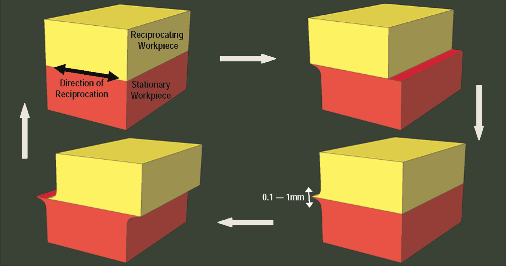
A schematic of a single cycle of the LFW process.
Detailed past investigations of the LFW process1–4 identified five distinct phases of this joining process. The first four LFW process phases, that is, (a) initial phase, (b) transition phase, (c) equilibrium phase, and (d) deceleration/forging phase, are depicted schematically in Figure 2. The fifth LFW process phase, that is, (e) the stand phase, is not shown since it does not involve workpiece length-scale structural/kinematic effects. Details regarding the main features of the five LFW process phases can be found in our prior work. 6
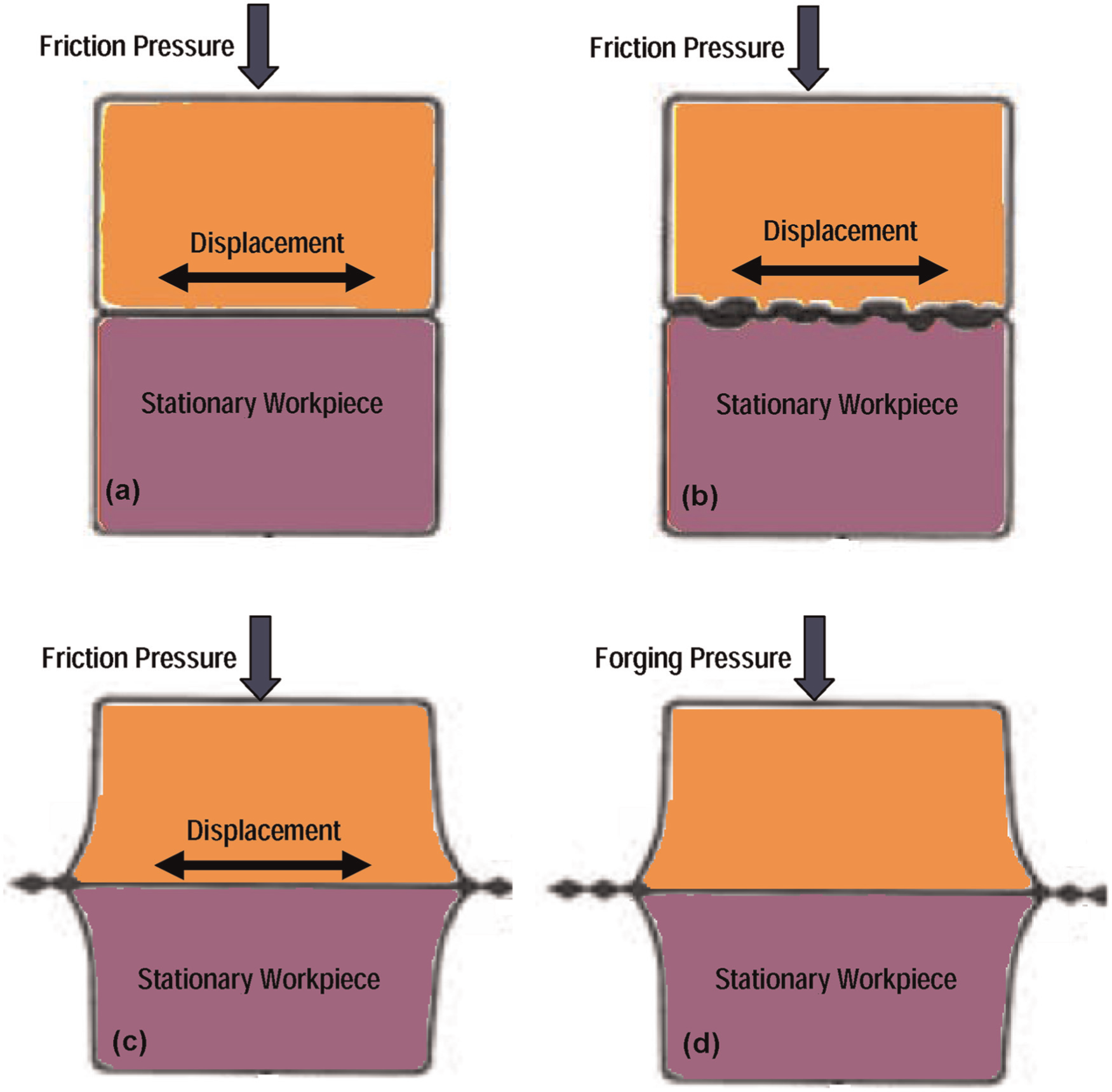
Schematic representation of the first four phases of the LFW process: (a) initial phase, (b) transition phase, (c) equilibrium phase, and (d) deceleration/forging phase.
LFW is characterized by the following main process parameters: (a) alloy grade and thermal–mechanical treatment of the workpiece materials to be joined, (b) reciprocating frequency, (c) reciprocating amplitude, (d) variation in contact/upsetting/forging pressure with time, (e) process duration, and (f) interfacial geometry and topography. It is generally found, and this work confirmed that the structural integrity and overall quality of the resulting weld may be strongly influenced by the selection of these parameters (or more precisely their combination).
Being one of the solid-state, friction-based welding processes, LFW offers several important advantages over the conventional fusion-welding technologies. Among these advantages, the most noteworthy are as follows: (a) no melting and re-solidification phenomena within the weld, that is, the phenomena that often compromise weld quality, accompany the process; (b) a greatly reduced thickness of the (property-degraded) heat-affected zone (HAZ) since the heat source is largely confined to the faying surfaces; (c) the capability to join high-performance, dissimilar metallic materials that are difficult to join using conventional welding processes. For example, LFW is a preferred method for joining aircraft-engine blades to disks (high-temperature structural components). The former are typically made of metallic materials with superior high-cycle fatigue properties, while manufacture of the latter typically requires the use of metallic materials with superior low-cycle fatigue properties. 7 (d) An attractive combination of enhanced mechanical weld properties and low weldment distortion; (e) absence of an external heat source; (f) typically, high reciprocating axial speeds are not required; (g) improved operator safety since neither toxic fumes nor molten material is produced; (h) amenability to control and automation; (i) relatively environmentally friendly; and (j) suitable, and often preferred, for welding non-metallic materials (e.g. plastics).
It is also important to note that the LFW process suffers from several important shortcomings/limitations. Among these, the most noteworthy are as follows: (a) joining is accompanied by flash formation. Flash contains the workpiece material that was originally located at the faying surfaces or in regions adjacent to them and was subjected to high temperature and the loss of strength and expelled/extruded in the course of welding. Since flash removal from the weldment adds a new manufacturing process step, it is associated with an increase in cost. (b) The process is limited to workpiece materials that (1) possess relatively low thermal conductivity and (2) possess relatively high strength in shear at elevated temperatures. (c) Control systems required for process automation are typically quite complex and high precision. (d) The process entails the employment of stiff fixturing systems with high capacity and large-capacity (typically hydraulic) loading systems.
Given the high cost of employing LFW, this process is mainly employed to join aircraft-engine components, the high value of which justifies the cost. For example, joining a blade and disk using LFW remains more cost-effective than machining the blade/disk (blisk) assembly from a single billet. New applications of LFW have been found in automotive, spacecraft construction, tool manufacturing, pipeline construction, and other energy-related industries.
Current state of knowledge as related to LFW
The current state of knowledge of LFW has been obtained mainly via (real-time or post-mortem) empirical/experimental investigations. Examination of the open-domain literature carried out as part of this work identified a number of investigations dealing with weldability, weld quality, and relationships between the LFW process parameters and the weld microstructure/properties in a variety of metallic materials/grades such as (a) titanium alloys,8–11 (b) superalloys, 12 (c) steels,13,14 and (d) intermetallics. 15 These investigations cumulatively established that the welding efficiency, spatial distribution and temporal evolution of material deformation and as-welded microstructure, and quality/structural integrity of the weld are all influenced by the interfacial temperature, which is the most significant process parameter.
The work presented in this article deals with LFW of Carpenter Custom 465 H1000, a high-strength/high-corrosion resistance PH martensitic stainless steel. Examination of the public-domain literature did not reveal any information regarding LFW of this material. The material closest to Carpenter Custom 465 for which an experimental LFW investigation has been reported is AISI 316L, a low-carbon austenitic stainless steel. 16 The investigation reported in Bhamji et al. 16 established that (a) with a proper choice of the LFW process parameters, structurally sound linear friction welds can be produced in AISI 316L, with tensile properties exceeding those of the base metal; (b) the LFW process has been found to be quite robust, displaying very little sensitivity of the weld structural soundness and mechanical properties to the selection of the process parameters; (c) in addition to the commonly found effects of the welding process on the weld-material grain structure/size, the formation of a {{1 1 1}} <1 1 2> -type crystallographic texture (often found in face-centered cubic (FCC) metallic materials subjected to shear strain–dominated plastic deformation) is also frequently observed; and (d) depending on the selection of the LFW process parameters, other changes in the weld-material microstructure were observed. For example, the volume fraction of δ-ferrite in the as-welded microstructure has been found to be mainly affected by the so-called burn-off rate, that is, by the rate at which plasticized material is expelled from the contact region. Specifically, when the burn-off rate is high and the material adjacent to the contacting interfaces is only briefly subjected to high temperatures, the thermo-mechanically affected zone (TMAZ) contains very little or no δ-ferrite. High burn-off rates are generally attained by combining high welding pressure with mid-range amplitudes (ca 1.5 mm) and frequencies (ca 30 Hz) of reciprocating motion.
Past LFW modeling and simulation efforts
While the experimental investigations overviewed in the previous section helped establish relationships between LFW process parameters and the as-welded material microstructure and properties, they mainly employed post-mortem (often destructive) microstructure/property characterization techniques. In addition, these efforts were less successful in generating real-time data as related to the material microstructure evolution during the LFW process or to the LFW process itself. For example, apart from the difficulty of measuring the temperature fields during the process, the uncertainty in these measurements was significant. 17 To overcome these limitations of the purely empirical approaches, considerable effort in recent years has been devoted toward developing computational techniques for simulating the evolution of the thermal, mechanical, and microstructural fields during the LFW process. A few of the most noteworthy past LFW process modeling and simulation efforts are overviewed in the remainder of this section.
Among the recent LFW process modeling and simulation efforts, the ones which appear most relevant to this investigation are as follows:
The work of D’Alvise et al., 18 in which a two-dimensional fully coupled thermo-mechanical finite element model of the LFW process was developed. In their work, flash formation was simulated using an innovative adaptive contact and re-meshing algorithm. The results (pertaining to the spatial distribution and temporal evolution of temperature and plastic deformation) yielded by the model displayed a reasonable level of agreement with their experimental counterparts.
In the work of Sorina-Müller et al., 4 a three-dimensional fully coupled thermo-mechanical finite element model for the LFW process was developed and subsequently applied to the case of Ti-6Al-2Sn-4Cr-6Mo alloy LFW joining. The computed results (pertaining to the evolution of the axial shortening and the variation in the as-welded material microstructure in the course of joining) yielded by the model were found to be in very good agreement with their experimental counterparts.
Grujicic et al. 6 extended the model of Sorina-Müller et al. 4 in order to provide a deeper insight into the development of material microstructure (and the associated mechanical properties) within different weld regions of Ti-6Al-4V and their dependence on the LFW process parameters. Specifically, since the HAZ of the weld has been found to possess somewhat inferior mechanical properties relative to the TMAZ and the base metal, particular attention has been given to the problem of establishing processing/microstructure/property relations in this weld region. The model predictions and their experimental counterparts pertaining to the overall structural performance of the LFW joint are found to be in reasonably good agreement.
Grujicic et al.5,6 extended their LFW process model described above to Carpenter Custom 465, a material that is the subject of this investigation. However, the extension was limited to the thermo-mechanical aspects of the LFW process model and not to the aspects of weld microstructure, temporal evolution, and spatial distribution. The latter aspects of the Carpenter Custom 465 LFW process model are the subject of this work.
Main objectives
The main objectives of this work are as follows: (a) to construct a microstructure-evolution model for LFW of Carpenter Custom 465, H1000, a high-strength/high-corrosion resistance, PH martensitic stainless steel (frequently employed in aircraft frames fabricated using LFW). During the construction of the microstructure-evolution model, key physical metallurgy concepts and principles of the subject material, and the basic thermodynamic and kinetic relations for various interacting and competing phase transformations which may take place within the weld region, will be utilized. (b) To combine this model with our recently developed fully coupled thermo-mechanical finite element–based LFW process model 5 for the same material in order to predict the type, the extent and the temporal evolution and spatial distribution of microstructural changes within different portions of the weld. (c) Through the combined use of the thermo-mechanical process model and the workpiece material microstructure-evolution model, it is planned to establish the basic functional relationships between the LFW process parameters (e.g. friction pressure, reciprocation amplitude, reciprocation frequency, and forging pressure) and the temporal evolution and the spatial distribution of the as-welded material microstructure.
Organization of this article
The fully coupled thermo-mechanical finite element LFW process model developed in our recent work 5 has been briefly overviewed in section “Thermo-mechanical LFW process model.” The key physical metallurgy aspects of Carpenter Custom 465 are presented in section “Physical metallurgy of Carpenter Custom 465.” Details regarding the development and parameterization of the LFW microstructure-evolution model are discussed in section “Carpenter Custom 465 weld microstructure model.” The main computational results obtained are presented and discussed in section “Results and discussion.” The key conclusions resulting from this study are summarized in section “Summary and conclusion.”
Thermo-mechanical LFW process model 5
In this section, a brief description is provided of our recently developed fully coupled thermo-mechanical finite element–based LFW process model. 5 In addition, examples of a few typical results yielded by the model are presented and briefly discussed. The two main aspects of the model are related to the (a) LFW process kinematics and mechanics and (b) the constitutive thermo-mechanical behavior of the workpiece material(s). These two aspects of the model are presented below in separate sections.
LFW process kinematics and mechanics
To construct the kinematic/mechanics portion of the LFW process model, the following aspects of the model had to be specified: (a) computational domain and its meshing; (b) computational analysis type; (c) initial conditions; (d) boundary conditions; (e) contact interactions; (f) heat generation and partitioning; (g) numerical formulation and algorithm; and (h) computational accuracy, stability, and cost.
Computational domain and its meshing
The computational domain employed in this work comprises two stacked workpieces initially shaped like rectangular parallelepipeds (Figure 1(a)). The two workpieces are allowed to reciprocate in the (shorter) y-direction, that is, in the direction of the shorter lateral dimension of the workpieces (in order to facilitate expulsion of the plasticized material and flash formation).
The two workpieces are meshed using thermo-mechanically coupled, reduced-integration finite elements. To ensure lower cost, accurate, and robust computational analyses, non-uniform meshes are used with small-size finite elements employed in the region surrounding the faying surfaces. The size of the smallest element was selected in accordance with the steepest local thermal gradient and the stability requirements of the explicit computational analysis used.
Computational analysis type
The LFW process is simulated using a fully coupled thermo-mechanical finite element algorithm.19,20 In the heat conduction equation, the heat dissipation associated with workpiece–workpiece interfacial friction sliding and plastic deformation is modeled as a heat source. To account for the effect of temperature on the mechanical response of the workpiece material(s) during joining, the material properties are all made temperature dependent.
Initial conditions
The thermo-mechanical analysis of the LFW process is carried out by assuming that the workpieces are at rest, stress-free, and at room temperature at the start of the simulation.
Boundary conditions
Due to the thermo-mechanical character of the analysis, both thermal and mechanical boundary conditions had to be specified. Thermal boundary conditions are defined by applying forced convection conditions (caused by the attendant reciprocating motion of the workpieces) and radiation conditions to all exposed surfaces (including the temporarily exposed portions of the faying surfaces). As far as the mechanical boundary conditions are concerned, the lower workpiece is made stationary by fixing its bottom nodes, while the top workpiece is subjected to a reciprocating motion by prescribing a time-dependent sinusoidal tangential displacement to its top nodes.
Contact interactions
Penalty contact is used to model the workpiece–workpiece normal interactions. Within this algorithm, the extent of penetration between the faying surfaces controls the magnitude of the contact pressure. A modified Coulomb friction law, which can account for the occurrence of the slip/stick phenomena, is used to model the tangential workpiece–workpiece interactions (responsible for the shear stress transmission across the interface). To properly account for the fact that the magnitude of the friction coefficient is controlled by the competition between processes leading to micro-weld formation and their shear fracture, functional relationships between the friction coefficient and (a) the (mean) temperature at the interface, (b) the contact pressure, (c) the slip speed at the interface, and (d) the roughness/topology of the contact surfaces are derived and parameterized for Carpenter Custom 465.
Heat generation and partitioning
Heat is assumed to be generated by (a) frictional sliding. In this case, it is the product of the local interfacial shear stress and the slip speed that controls the rate of heat generation and (b) dissipation of the work of plastic deformation.
Heat generated by the two aforementioned sources is partitioned between the two workpieces in accordance with the fact that (a) the distance traveled by the heat wave front from the contact interface scales with the square root of the workpiece material thermal diffusivity, while (b) the heat per unit volume of the workpiece material associated with an increase in temperature by 1 °C scales with the product of the material mass density and its mass-based specific heat.
Numerical formulation and algorithm
To overcome potential numerical problems associated with highly distorted elements in the region surrounding the contact interface, an arbitrary Lagrangian–Eulerian (ALE) formulation is used. Within this algorithm, a good-quality mesh was maintained by means of adaptive re-meshing. To solve the fully coupled thermo-mechanical ALE problem at hand, a second-order accurate, conditionally stable, explicit algorithm implemented in ABAQUS/Explicit, 21 a general-purpose finite element solver, is used.
Computational accuracy, stability, and cost
To keep the computational cost reasonable while ensuring accuracy and stability of the computational procedure, mesh sensitivity and mass-scaling procedures are employed. The mesh sensitivity procedure ensures that further mesh refinement, which is accompanied by an increase in the computational cost, does not significantly improve the accuracy of the results. On the other hand, the mass-scaling algorithm adaptively adjusts material density in the critical (time increment controlling) finite elements, to increase the critical time increment without significantly affecting the computational accuracy.
Material models
The thermo-mechanical LFW process model developed in Grujicic et al. 5 and its microstructure-evolution counterpart, developed in this work, deal with the case of the two workpieces to be welded being made of the same material, Carpenter Custom 465, in the slightly overaged H1000 condition. The mechanical behavior of this material is assumed to be of an elastic/plastic character. The elastic response of the material is assumed to be isotropic, linear, and temperature dependent and to be governed by a generalized Hooke’s law. As far as the plastic response of the material is concerned, it is assumed to be strain-hardenable, strain rate–sensitive, and thermally softenable and to be described by the Johnson and Cook 22 material model. This model is generally found to be capable of accounting for the material behavior under large-strain, high deformation rate, high-temperature conditions, the type of conditions commonly encountered in the problem of computational modeling of the LFW process. The thermal and thermal–elastic behavior of Carpenter Custom 465 is assumed to be of an isotropic and temperature-dependent character. Consequently, the thermal/thermo-mechanical model is fully defined by the following three temperature-dependent parameters: (a) thermal conductivity, (b) specific heat, and (c) thermal expansion coefficient. Parameterization (including temperature dependence) of the complete material model for Carpenter Custom 465, H1000, is carried out using a multiple regression analysis of the reported experimental data and by employing different property-correlation procedures.
Physical metallurgy of Carpenter Custom 465
Introduction to the material
As mentioned earlier, the material analyzed in this work is the premium (i.e. double vacuum) melted Carpenter Custom 465 PH martensitic stainless steel (UNS S46500). Stainless steels are a class of ferrous alloys characterized by a superior combination of oxidation resistance and corrosion resistance. In these alloys, improved oxidation resistance is typically achieved through the addition of chromium (minimum ca 12 wt%), which ensures the formation of a continuous Cr2O3-based oxide protective surface film (with low-oxygen permeability and high adhesion strength). Enhanced corrosion resistance, on the other hand, is typically achieved by ensuring, through the chemical composition and heat treatment, that the alloy contains only one crystalline phase. Depending on the nature of that phase, the following three classes of stainless steels are defined: (a) austenitic, (b) ferritic, and (c) martensitic. In other classes of stainless steels, the requirement for increased fracture toughness and the enhanced retention of mechanical properties at high temperatures demands the introduction of a secondary phase. When the secondary phase is introduced through an aging treatment, the resulting stainless steel is classified as a PH stainless steel. Carpenter Custom 465 falls into this class of stainless steels. In addition, in order to denote that the parent phase from which precipitate formation takes place is martensite, Carpenter Custom 465 is typically referred to as a PH martensitic stainless steel. In PH stainless steels, in order to reduce the tendency for dissimilar-metal corrosion between the matrix and the precipitates, only intermetallic precipitates like Ni3Al, Ni3Ti, Ni3 (Al, Ti), NiAl, Ni3Nb, Ni3Cu, and Laves phase 23 are allowed. This ensures that the electro-negativity difference between the two phases is relatively small and the associated dissimilar-metal corrosion rate is low.
While Carpenter Custom 465 was originally developed for use in the aerospace industry, it offers a good combination of properties of interest to a wide variety of applications. The benefits offered by Carpenter Custom 465 could be fully understood by recognizing that in today’s highly competitive business climate, among the materials that offer the required performance, those are often selected, which are associated with a low total life cycle (TLC) cost rather than those having a low initial cost of acquiring. This paradigm shift created a strong demand for high-performance materials, such as Carpenter Custom 465, which could be readily fabricated into complex structural components capable of offering high reliability and durability even under severe corrosive environments. This is the reason that despite its higher initial cost relative to those of alternative stainless and alloy steels such as 15-5PH, 13-8, Type 4340, and 300M, Carpenter Custom 465 has found a wide use in various end-use markets such as aerospace, automotive, medical, oil and natural gas, consumer, and sporting equipment industries.
Chemical composition
Carpenter Custom 465 has the following nominal chemical composition expressed in wt%: C: 0.02; Mn: 0.25; P: 0.015; S: 0.01; Si: 0.25; Cr: 11.0–12.5; Ni: 10.75–11.25; Mo: 0.75–1.25; Ti: 1.5–1.8; and Fe: 72.65–75.45. This chemical composition along with the appropriate thermo-mechanical heat treatment (described below) is responsible for the superior combination of high strength and high corrosion resistance found in Carpenter Custom 465.
Due to its superior corrosion resistance, Carpenter Custom 465 usually does not require the use of chromium-, nickel-, or cadmium-protective (typically electroplated) coatings. Since the use of protective coatings increases both the initial cost (due to introduction of additional manufacturing process steps) and the TLC cost (coated structures must be periodically inspected to ensure coating integrity and this is generally associated with the equipment downtime), Carpenter Custom 465 is favored in many applications despite its relatively high initial cost. Furthermore, the electroplating process as well as the disposal of the coating-process waste chemicals often must meet very strict environmental regulations. For example, the US Environmental Protection Agency (EPA) and the environmental agencies of the European Union continue to tighten environmental regulations related to the use, emission, and disposal of harmful chemicals (in particular, cadmium) to the environment. While currently cadmium-based coatings are not completely banned, future restrictions and regulations may make the disposal cost of cadmium-coated components and the associated electroplating equipment prohibitively high.
Heat treatment(s)
To obtain the best combinations of mechanical and environmental resistance properties for a given application, Carpenter Custom 465 is either given a solution-annealing heat treatment (heat treatment designation A) or a solution-annealing plus precipitation-hardening treatment (heat treatment designation H). These two heat treatments are briefly described in the following.
Solution-annealing heat treatment
Within this heat treatment procedure: (a) the as-received microstructure of the material is first fully austenitized by exposing the material to a sufficiently high temperature, typically 1255 K ± 8 K (982 °C ± 8 °C), for a sufficient amount of time, typically 1 h; (b) diffusion-type decomposition of the resulting austenite is prevented during subsequent cooling to room temperature through the application of quenching-based high cooling rates; and (c) since the temperature for start of the martensitic transformation, the so-called Ms temperature, is above the room temperature, the as-quenched material microstructure obtained in (b) consists of untransformed martensite and untransformed austenite. To complete the transformation of austenite into martensite, the as-quenched material is, within a time period of less than 24 h following the solutionizing treatment, subjected to a refrigeration treatment at 196 K (−77 °C) for about 8 h. This temperature is lower than the martensitic transformation finish temperature, the so-called Mf temperature, and drives the austenite → martensite phase transformation to (near) completion. Subsequently, the material is allowed to warm up to room temperature. This step of the solution-annealing heat treatment is normally referred to as the cold-treating step. The main purpose for completing austenite → martensite phase transformation in the condition A of Carpenter Custom 465 is to achieve the required level of the material strength. In the case of the condition H of this material (presented below), on the other hand, the lath-type martensitic morphology (through the presence of numerous lath interfaces and intra-lath dislocations) provides an abundance of potential nucleation sites for the precipitation phase(s). This, in turn, ensures that during the subsequent aging treatment, the resulting microstructure will contain a high number density of very fine (material-strength/toughness-enhancing) precipitates.
Age-hardening heat treatment
To place Carpenter Custom 465 into the condition H, this material in condition A is subsequently subjected to an age-hardening heat treatment. This heat treatment process involves one-step artificial aging of the solution-treated plus cold-treated material in a temperature range between 755 K and 894 K (482 °C and 621 °C) for 4–8 h. This is followed by a water quench treatment (required in the case of section thickness exceeding ca 75 mm) or by air-quench treatment of the material. The resulting as-aged material condition is designated as Hxxxx where xxxx is replaced with the aging temperature expressed in °F (e.g. H1000 denotes a 1000°F age-hardening heat treatment). As will be shown below, the choice of the age-hardening heat treatment temperature gives rise to a trade-off in material properties such as strength, fracture toughness, notch sensitivity, and stress corrosion cracking (SCC) resistance. For example, an increase in the age-hardening temperature lowers material strength but increases toughness.
Precipitation reaction(s) during aging
It should be first noted that relatively little has been reported in the open literature regarding the details of the precipitation reaction(s) during aging. The summary presented in this section is based both on the reports dealing specifically with Carpenter Custom 46524–26 and reports dealing with steels with comparable chemistry to that of Carpenter Custom 465.27,28 The main microstructural changes occurring in Carpenter Custom 465 during aging are associated with the formation of coherent hexagonal crystal-structure (a = 0.4058 nm, c = 0.2485 nm) 27 needle-shaped ω-phase metastable precipitates and their ultimate replacement with incoherent orthorhombic-structure plate-like Ni3(Ti,Mo)-phase equilibrium precipitates. Due to coherency between the ω-phase and the matrix, initial formation of small ω-phase precipitates is thermodynamically favored over the equilibrium Ni3(Ti,Mo) phase. However, as the ω-phase particles acquire a larger size, coherency gives rise to a large energy increase in the ω-phase precipitates and the thermodynamically favored Ni3(Ti, Mo)-phase precipitates begin to form and replace previously formed precipitates of the ω-phase. It should be also noted that there may be another fundamental difference in the precipitation process of the two phases. 28 That is, while the equilibrium Ni3(Ti,Mo)-phase precipitates form by the standard diffusion-based atomic clustering and reordering mechanism, ω-phase precipitates are believed to form through either a concurrent or sequential operation of athermal displacive and diffusion-based replacive processes. Since the athermal processes are associated with high rates (comparable to the speed of sound), initial formation of the ω-phase is also kinetically favorable.
Typically, Carpenter Custom 465 acquires its peak strength/hardness before precipitates of the ω-phase and Ni3(Ti,Mo) phase become visible under a light optical microscope. Submicron-size coherent ω-phase precipitates introduce lattice distortions into the surrounding martensitic matrix, and this phenomenon is believed to be the main aging-induced strengthening mechanism in this class of alloys. As mentioned above, as the aging process continues, ω-phase transient coherent precipitates are gradually replaced with Ni3(Ti,Mo) equilibrium incoherent precipitates, and this change in the material microstructure gives rise to a loss of strength and, initially, an improvement in material fracture toughness. It should also be noted that at sufficiently high aging temperatures, (undesirable) martensite → austenite reversion may take place, giving rise to an increase in material ductility and a substantial loss in its strength. Typical microstructure of Carpenter Custom 465 in an aged condition close to the peak-strength condition is shown in Figure 3. 24 This microstructure is fully dominated by lath martensite, that is, precipitates are not visible (due to their submicron size), and reverted austenite is absent (since the aging temperature was too low for the martensite → austenite transformation to take place).
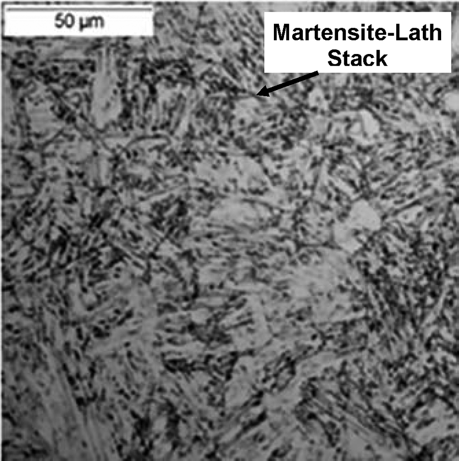
Optical micrograph showing a typical lath martensite dominated microstructure of Carpenter Custom 465 in an aged condition close to the peak-strength condition. Strength-controlling precipitates are not visible at the magnification employed.
Material-property trade-offs
As mentioned above, systematic variations in the age-hardening temperature typically yield trade-offs in material strength, fracture toughness, and SCC resistance. This is clearly seen in Figure 4(a)–(c), which shows that as the aging temperature increases, material strength decreases (Figure 4(a)), while its fracture toughness (Figure 4(b)) and SCC resistance (Figure 4(c)) increase. Most frequently, Carpenter Custom 465 is used in either its H950 or H1000 condition.
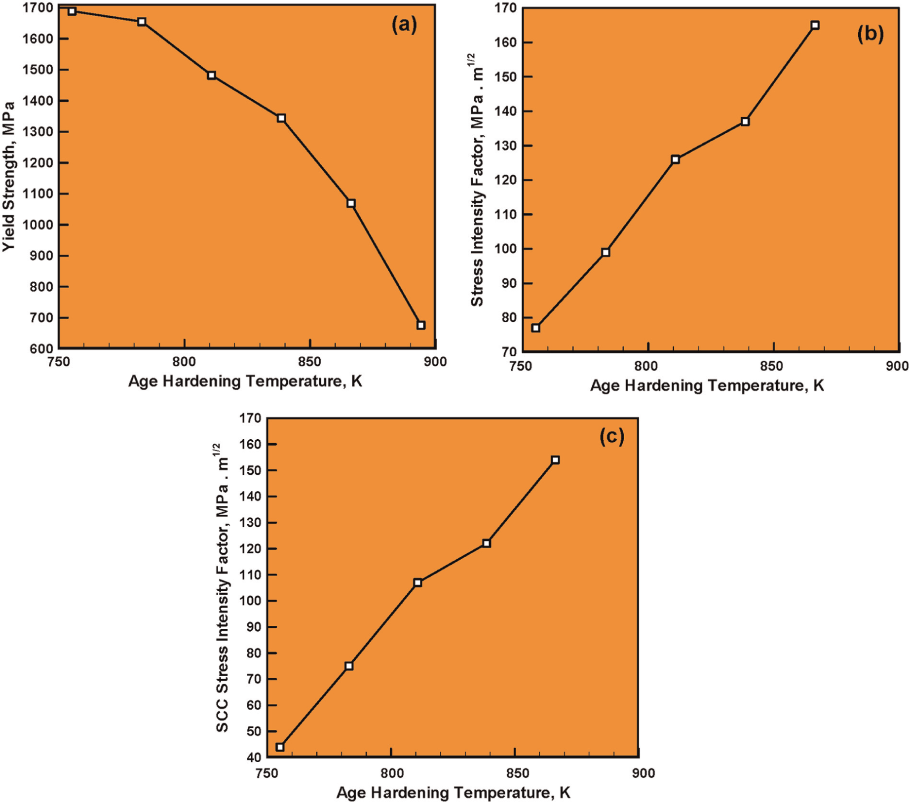
Effect of aging treatment (for 1 h at different temperatures) on the material: (a) yield strength, (b) fracture toughness, and (c) SCC resistance at room temperature in Carpenter Custom 465 (previously solution-annealed and cold-treated).
Comparison to other PH martensitic stainless steels
In its H950 condition, Carpenter Custom 465 can acquire tensile strength as high as 1724 MPa, a level that is higher than that found in any other PH stainless steel (long product). This is evidenced by the results displayed in Table 1 and Figure 5.
A comparison of typical properties of several high-performance PH stainless steels. 24
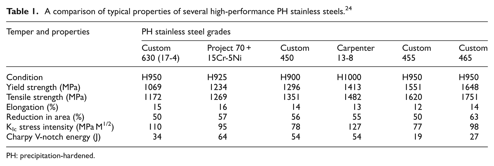
PH: precipitation-hardened.
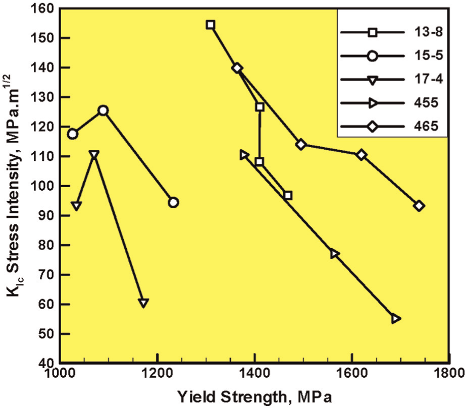
Fracture toughness/strength trade-off in several Carpenter high-performance stainless steels, including Carpenter Custom 465.
The results displayed in Table 1 referred to typical mechanical properties of Carpenter Custom 465 and the competing PH martensitic stainless steel alternatives. Figure 5, on the other hand, shows the aforementioned fracture toughness/strength trade-off in five Carpenter high-performance PH martensitic stainless steels (including Carpenter Custom 465). It is seen that over the entire range of material strengths covered, Carpenter Custom 465 has the best combination of strength and fracture toughness. It should also be noted that the use of cold-working prior to the H950 age-hardening heat treatment can result in tensile strength values as high as 1930 MPa (280 ksi).
Corrosion resistance
Relative to general corrosion, the resistance of Carpenter Custom 465 is comparable to that observed in a prototypical austenitic stainless steel such as Type 304 stainless steel. Specifically, in both the H950 and H1000 conditions, Carpenter Custom 465 does not show any sign of corrosion after exposure for 2000 h to 5% neutral salt spray at the temperature of 35 °C (308 K).
Carpenter Custom 465 also possesses a respectable level of the SCC resistance (as quantified by the corresponding Mode I stress intensity factor, KIscc). This is particularly true considering the superior strength properties offered by this material, as depicted in Figure 6. In this figure, the strength and SCC resistance properties are compared for several high-performance PH martensitic stainless steels including Carpenter Custom 465. Superior SCC resistance of Carpenter Custom 465 is specifically demonstrated by the results of the rising step load (RSL) tests conducted under 3.5% NaCl solution, natural pH, and open-circuit potential conditions. These results revealed KIscc = 0.75 KIc for H950 condition and KIscc = 0.9 KIc for H1000 where KIc represents the corresponding in-air stress intensity factor.
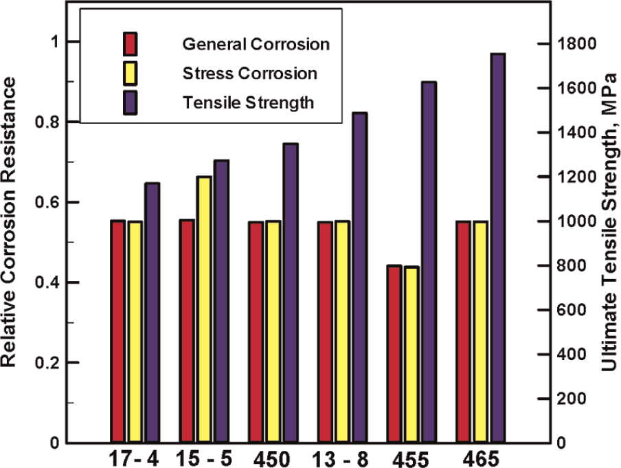
A comparison of the relative general and stress corrosion resistances and the ultimate tensile strength of several Carpenter high-performance stainless steels.
Weldability
As mentioned earlier, while Carpenter Custom 465 is commonly welded in the aerospace industry using LFW, there are no public-domain reports describing LFW behavior of this material. This material is also often welded using gas tungsten arc (GTA) and gas metal arc (GMA) welding processes, with no workpiece heating required. In the case of GTA, a matching filler metal can be used, while in the case of (high heat input) GMA, Pyromet® X-23 alloy must be used as a filler metal to prevent weld-bead cracking. Oxyacetylene welding is generally not recommended due to potential carbon pickup during the course of welding. In principle, Carpenter Custom 465 can be successfully welded using the aforementioned fusion-based welding processes in either solution annealed/cold-treated or age-hardened conditions. However, welding may introduce significant spatial variations in material microstructure and, hence, properties such as strength/hardness, fracture toughness, notch sensitivity, and SCC resistance throughout the weld region. Restoration of the optimal microstructure and properties within the weld region would typically require (if possible) application of the aforementioned heat treatments (solution-annealing, cold-treating, and age-hardening) to the entire weldment.
Applications
Carpenter Custom 465 was originally designed to help meet the demand from the aerospace industry for airframe materials that could enable aircraft to keep flying 30 years or more with minimal maintenance. Currently, Carpenter Custom 465 is used by major airframe manufacturers in structural applications such as torque tubes, pneumatic cylinders, braces, struts, and fuse pins. Other areas of applications of this material include the following: (a) medical—for example, for minimally invasive surgical instruments that can withstand higher operational torque loads and multiple autoclaving cycles; (b) energy—for example, for driveshafts in deep-hole drilling tools; (c) automotive—for example, for suspension coil springs, engine valve springs, and torsion bars; (d) sporting equipment—for example, for golf-club face-plates and wire face-shields for lacrosse helmets; and (e) hand tools—for example, conventional screwdrivers, L- and T-pattern hex keys, ball-end, and L-pattern hex keys.
Carpenter Custom 465 weld microstructure model
As mentioned earlier, the main microstructural changes occurring in Carpenter Custom 465 during aging are associated with the formation of coherent metastable ω-phase precipitates and their ultimate (undesirable) replacement with incoherent stable Ni3(Ti,Mo)-phase precipitates. In addition, at sufficiently high aging temperatures, (also undesirable) martensite → austenite reversion may take place. Typically, Carpenter Custom 465 is used in either its peak-strength H950 temper or its slightly overaged (improved fracture toughness and SCC resistance) H1000 temper. Exposure of Carpenter Custom 465 in either of these two aged conditions to high temperatures in the weld region surrounding the contact interface may, in principle, give rise to the undesirable aforementioned coherent-precipitate overaging/dissolution and austenite reversion microstructural changes.
In this section, details regarding the formulation and implementation of a multicomponent precipitate formation/overaging microstructure-evolution model are presented. In our prior Carpenter Custom 465 LFW process modeling work, 5 it was demonstrated that LFW process parameters can be selected in such a way that the formation of a sound, good-quality weld is ensured while the possibility of austenite reversion is minimal. Consequently, no attempt is made in this work to model the martensite–austenite reversion process. Furthermore, since the formation of coherent metastable ω-phase and incoherent stable Ni3(Ti,Mo)-phase precipitates, for the most part, takes place concurrently, precipitate formation and overaging are assumed to involve only one effective precipitate phase. The model could be easily extended to the case when concurrent and competing formation of two types of precipitates takes place, and this will be done in our future work. However, as will be shown below, the extent of thermodynamics and kinetics data needed to implement such a model is quite extensive and such data were not available for use in this work.
Model formulation
Precipitate formation during aging is one of the most important types of phase transformation processes in material systems since it may dramatically change a variety of material properties. The ability to predict (and, possibly, control) the microstructure of the precipitates within the LFW weld provides a powerful tool in the development of this joining process. Computational modeling of precipitate formation during aging has been an active research area in materials science for many years. Phase precipitation during aging typically involves three distinctive processes: (a) precipitate nucleation, (b) precipitate growth, and (c) precipitate coarsening/dissolution. Within the continuum framework, precipitation has been modeled using approaches of varying complexities (from the simplest single-variable Kolmogorov–Johnson–Mehl–Avrami type of models to highly complex multi-variable phase-field models) with the computational cost typically increasing exponentially with the complexity of, and the details captured by, the models.
Following the approach presented in Jou et al., 29 aging of the precipitates within the LFW weld is analyzed, in this work, using a two-variable continuum-type model. This model treats nucleation, growth, and coarsening in an integrated fashion and is based on the framework put forth in Langer and Schwartz 30 and its numerical implementation introduced by Kampmann and Wagner. 31 The two model variables are the precipitate/particle size and particle number density, and jointly they are used to define the particle size distribution (PSD). Knowledge of the PSD, in turn, enables the calculation of various precipitate-related microstructural parameters such as precipitate volume fractions, particle mean sizes, and inter-particle distances (all of which are used when one tries to predict mechanical properties of the LFW weld).
Successful modeling of the precipitation process using the numerical Langer–Schwartz–Kampmann–Wagner framework has been reported in the open literature.32–35 However, the alloy systems analyzed are all of a binary character and only the isothermal precipitation processes are considered. In the case of microstructure evolution within the LFW weld of Carpenter Custom 465, neither of these two conditions is satisfied. That is, the material under investigation is of a multicomponent character while precipitate aging takes place under highly non-isothermal conditions. Recently, however, Jou et al. 29 successfully expanded the numerical Langer–Schwartz–Kampmann–Wagner framework into the domain of multicomponent materials and non-isothermal aging processes. The approach presented by Jou et al. 29 is adopted and customized to Carpenter Custom 465 in this work. It should be noted that the main components of this model are as follows: (a) nucleation (source of new particles), (b) growth (particle size changes) under mean field, (c) time evolution of the PSD, and (d) species/mass conservation. Coarsening is not treated as a separate process but rather as an outcome of the interaction and competition between nucleation and growth processes. Furthermore, due to the natural integration of the aforementioned model components, no ad hoc interventions are needed to model distinctive aspects of the precipitation process. For example, the model is capable of capturing experimentally observed phenomenon related to the absence of the precipitate growth process in highly supersaturated alloy systems.
PSD function
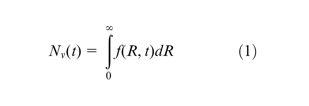
As mentioned above, the key quantity used in this model is the PSD function, f(R, t), which is defined such that f(R, t) dR represents the number of particles of size R to R + dR present per unit volume of the material at time t. For a given PSD function, one can readily define the number of particles per unit material volume, Nv , as
as well as the particle volume fraction, ϕ, as
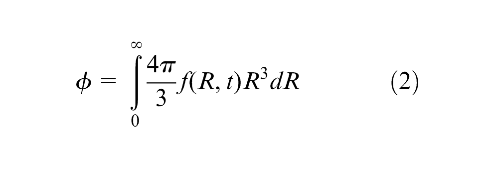
Continuity equation
Temporal evolution of the PSD function is governed by the following continuity equation
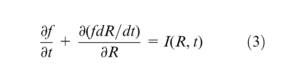
where
It should be noted that Equation (3) is a partial differential equation of the first order, and as such, must be accompanied by (a) one initial condition defining the PSD at t = 0, f(R, 0) and (b) one boundary condition that defines a functional relationship that f(R, t) must satisfy at any time t > 0. In addition, before one can attempt to solve equation (3), functional relationships for the growth
Precipitate growth rate model
Within the approach used in this work, precipitate growth is assumed to be controlled by (a) the surrounding diffusion fields and (b) the constraints associated with local equilibrium at the precipitate–matrix interface. In addition, the quasi-stationary approximation is adopted and the inter-diffusion coefficient is assumed to be independent of the chemical composition. It should be noted that in a multicomponent alloy system (in contrast to the binary systems), precipitate and matrix interfacial concentrations are not controlled by the phase diagram, but rather by the extent of super-saturation and the species diffusion coefficients. To improve fidelity of the precipitate growth model, the following effects must be included: (a) capillarity (i.e. particle-curvature) effects, (b) interfacial kinetics, and (c) precipitate non-zero volume fraction phenomenon. With all these effects included, the growth rate of a particle of size R can be defined as
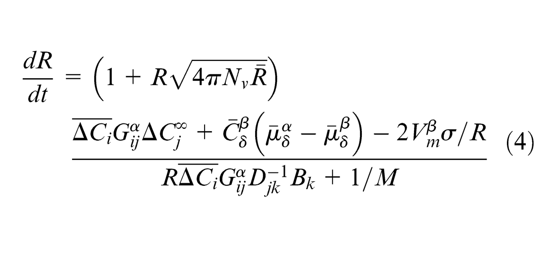
where (a) the sum over repeated Latin indices (denoting atomic species) (2,..., N) and repeated Greek indices (denoting phases) (1,..., N) is assumed; (b) N − 1 is the number of alloying elements; (c)
The effect of interfacial kinetics on the precipitate growth rate is accounted for by the 1/M term (as well as by the y term) appearing on the right-hand side of equation(4) and is based on the assumption that the precipitate–matrix interfacial velocity scales with the interfacial mobility and total chemical driving force on the interface. Temperature dependence of the interfacial mobility is expressed as M = M 0 exp(−Q/RgT) where M 0 is the prefactor, Q is the activation energy for interfacial kinetics, and T is the temperature.
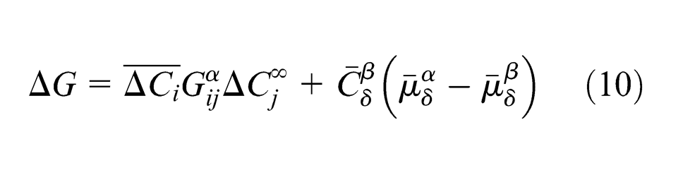
It should be noted that the chemical composition of the matrix phase about which the free energy is expanded affects the accuracy of the calculated precipitate growth rate, and hence, must be updated in the course of the precipitate-evolution analysis. However, in order not to compromise the computational speed, updating of the chemical composition is done adaptively rather than during each time step. It should be recalled that in contrast to the binary system, in which the precipitate growth rate, at a given temperature, is completely controlled by the extent of super-saturation, in multicomponent alloy systems (as is the present case), the precipitate growth rate is also affected by the second partial derivative of the Gibbs free energy, Gij . The reason for this difference lies in the fact that the concentrations at the precipitate–matrix interface in a multicomponent system are not fully defined by the local equilibrium conditions, but are also controlled by the species flux-balance requirements at the interface.
Critical size of nucleating precipitates
Examination of equations (4) and (8) reveals that when y = 0,
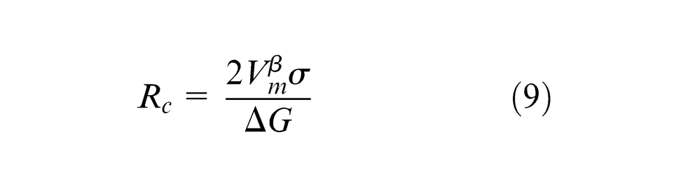
where
represents the free energy change on forming β of the composition of the critical nucleus from α of composition
Isothermal precipitate-nucleation rate
Under isothermal conditions, the rate of precipitate nucleation (including the incubation time effect) can be defined as
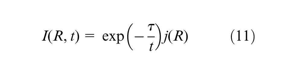
where τ is the incubation time and the nucleation-rate function j(R) is based on the assumption that the sizes of the nucleating precipitates follow a Gaussian distribution as
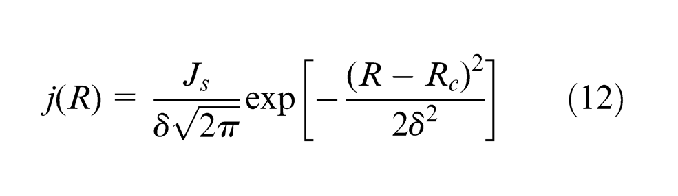
where Js is the total steady-state nucleation rate and δ is the variance of the particle size Gaussian distribution function. To ensure that only the nucleated precipitates with a size greater than Rc are included, the following relationship is imposed between j(R) and Js
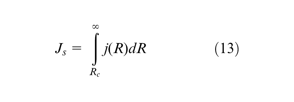
The total steady-state nucleation rate can be defined as
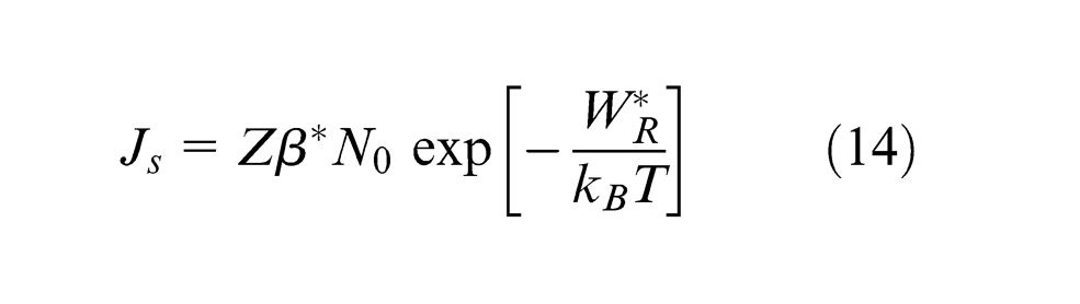
where Z is the Zeldovich factor (which accounts for the fact that the number density of critical precipitate nuclei is reduced due to finite probability for their shrinkage), β* is the rate of atom impingement onto the growing cluster/nucleus, N
0 is the number of atoms per volume,
The work associated with the nucleation of a precipitate of size Rc is defined as
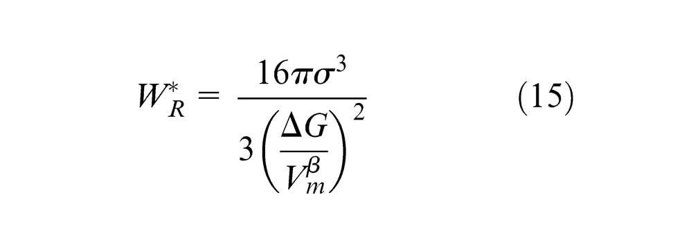
where ΔG is the volume free energy change on forming a nucleus of size Rc
, and
The Zeldovich factor is defined as
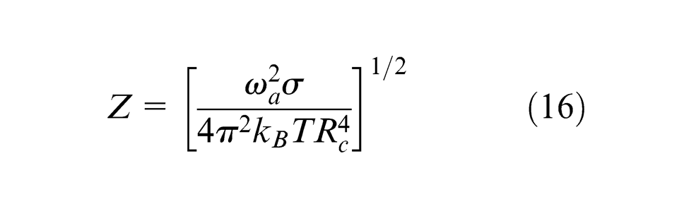
where ωa is the volume per atom in the matrix phase α.
As far as the impingement rate is concerned, its functional form depends on the rate-limiting mass transport process responsible for the precipitate nucleation. The two limiting regimes of the atom impingement process are as follows: (a) the regime in which the atom impingement process is controlled by the rate of atom transfer across the nucleus–matrix interface and (b) the regime in which the atom impingement process is controlled by the long-range atomic diffusion to the growing cluster/nucleus. In this work, only the second regime of the atom impingement process is considered. By solving the diffusion equation describing flux of solute atoms to a growing cluster, the slowest diffusing species and the associated cluster growth rate can be determined. Then the rate of atom impingement on the cluster–matrix interface can be defined as
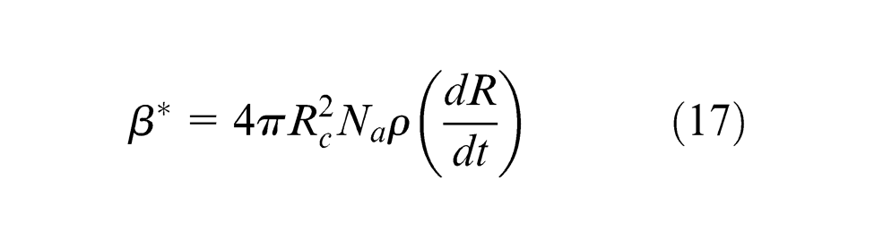
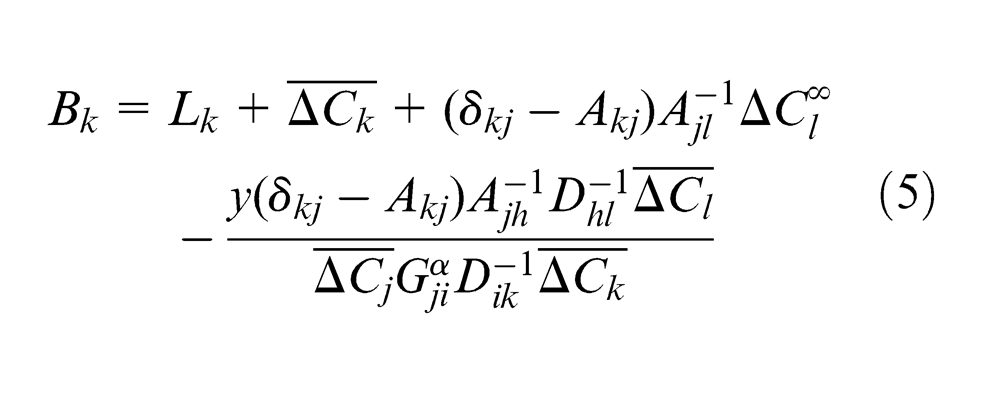
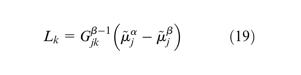
where ρ is the (constant) molar density of the material, Na is the Avogadro’s number, while the growth rate dR/dt is evaluated at the cluster critical size R = Rc . By expressing the growth rate in equation (17) using equation (4), while neglecting the interfacial energy proportional capillary effect term, the following equation is obtained
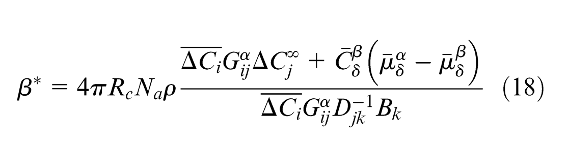
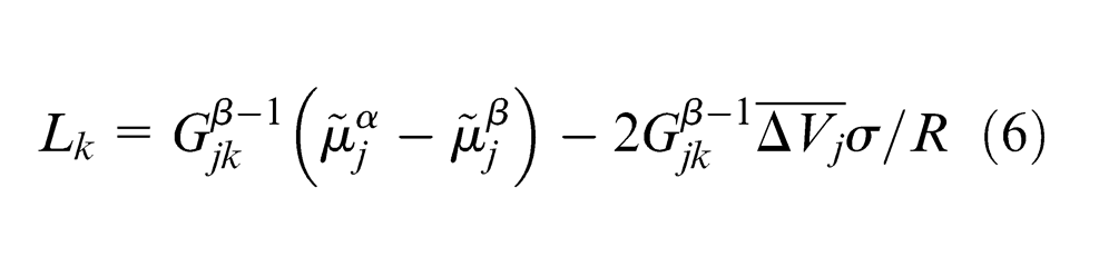
where Bk was given by equation (5) while, due to omission of the capillary effect term, Lk is redefined as
To complete the construction of the isothermal-precipitate nucleation model, the following expression for the diffusion-controlled incubation time is utilized
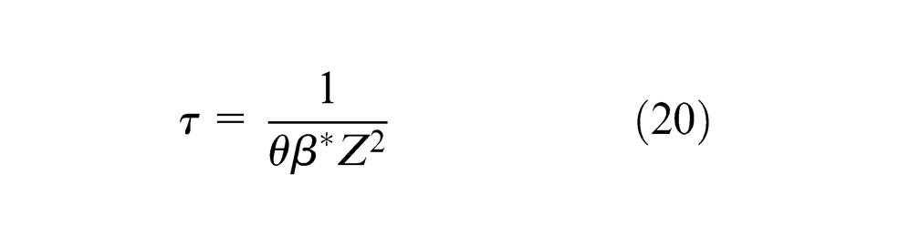
where 2π ≤ θ ≤ 4π.
Non-isothermal precipitate-nucleation rate
Under non-isothermal conditions, one can essentially use the same relations as those defined under isothermal nucleation conditions, after care is taken of the temperature dependence of the key parameters. Specifically, β * and Z, as defined, respectively, by equations (17) and (16), are already temperature dependent and no changes are required in the definition of these quantities. On the other hand, a new expression other than equation (20) is required to account for the non-isothermal nature of the nucleation process. Following the procedure proposed in Jou et al., 29 which replaces a more rigorous treatment based on the Fokker–Planck equation with a diffusion equation describing a random walk of the nuclei in cluster size space, the following integral equation is derived for the non-isothermal incubation time, τ

Mass conservation
The final functional relationship, which concludes the formulation of the Langer–Schwartz–Kampmann–Wagner precipitation model, involves the atomic species mass-conservation equations defined as
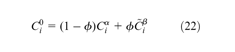
where
where f 2 is the second moment/variance of the PSD. Since equations (22) and (23) include the PSD function at time t, they provide the boundary condition required for the full definition of the continuity equation, equation (3).
Model implementation
Due to its complex multicomponent character, the governing continuity equation for the PSD, equation (3), cannot be solved analytically. Consequently, this equation had to be solved numerically by discretizing the PSD in the particle size versus time coordinate frame. This discretization is done in an adaptive fashion in order to ensure a good compromise between computational accuracy and efficiency. equation (3) is next solved numerically using the method of characteristics. 36 All the calculations in this portion of the work were done using MATLAB, a general-purpose mathematical package. 37
Numerical solution of equation (3), which yields temporal evolution of the PSD, entails the knowledge of the basic thermodynamic and kinetic/diffusivity parameters for the attendant crystalline phases and atomic species. These were assembled using various public-domain sources and validated using simple test procedures.
Results and discussion
It should be recalled that the main emphasis of the work presented in this article is the development of a LFW microstructure-evolution model for Carpenter Custom 465, H1000. The development of this model was presented in the previous section and the results yielded by the model will be presented and discussed in the last portion of this section. However, prototypical results yielded by the previously developed thermo-mechanical LFW process model 5 are presented and discussed first. This is done for the following reason: some of the output results from the LFW thermo-mechanical process model (e.g. temperature fields and plastic deformation fields) are used as input into the newly developed LFW microstructure-evolution model.
Typical results yielded by the LFW thermo-mechanical process model
The results yielded by the LFW thermo-mechanical process model are divided into the following three groups: (a) spatial distribution and temporal evolution of the interface temperature and the temperatures of the material points surrounding the interface, (b) temporal evolution and geometry of the expelled material/flash, and (c) temporal evolution of the axial shortening. In the remainder of this section, prototypical results from each group are presented and discussed. It should be noted that unless stated otherwise, the results presented in this section are obtained under the following LFW process conditions:
Initial, transition, and equilibrium phases
Friction amplitude = 2 mm
Reciprocation frequency = 50 Hz
Friction time = 1.8 s
Friction pressure = 150 MPa
Deceleration/forging phase
Forge time = 3.6 s
Forge pressure = 200 MPa
Stand phase
Post-forge time = 18 s
Spatial distribution and temporal evolution of the interface temperature
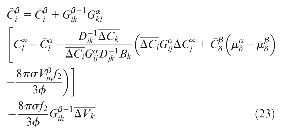
From the standpoint of obtaining a sound weld with good mechanical properties, temperature uniformity over the contact interface as well as the maximum value of the interface temperature attained during the course of the LFW process is of major concern. This is the main reason that temperature uniformity and maximum interface temperature, during LFW, must be monitored and analyzed. An example of typical results pertaining to the temperature (K) distribution over the contact interface within the LFW equilibrium phase is displayed in Figure 7(a). The results displayed in this figure show that there is a (undesirable) temperature difference between the central region of the contact interface and the interface edges, which is caused by the periodic loss of contact between the faying surfaces over edge regions, which extend orthogonally to the direction of reciprocation. The width of these edge regions is approximately equal to the reciprocating amplitude. In these regions of the contact interface, temperatures are lower for two main reasons: (a) heat is not being generated and (b) heat is being lost via convection and radiation while these regions are being exposed, that is, not in contact. The results displayed in Figure 7(b) show that the extent of the aforementioned temperature non-uniformity is controlled by the LFW process parameters such as the friction contact pressure and the reciprocation frequency.
(a) Typical temperature (K) distribution over the contact interface during the equilibrium phase of LFW of Carpenter Custom 465, H1000, and (b) the effect of the contact pressure and reciprocation frequency on the maximum temperature difference (K) over the contact interface during the equilibrium phase of LFW of Carpenter Custom 465, H1000, at a constant level of the reciprocation amplitude of 2 mm.
The second aspect of the interface temperature is its maximum value attained during the LFW process. This value must not exceed not only the material’s solidus temperature but also the substantially lower austenite reversion (AS ) temperature (estimated as 1045 K for Carpenter Custom 465, H1000). As will be shown later in this section, even tighter maximum interfacial temperature requirements might be necessary due to the overaging tendency of (and the associated loss of strength in) Carpenter Custom 465.
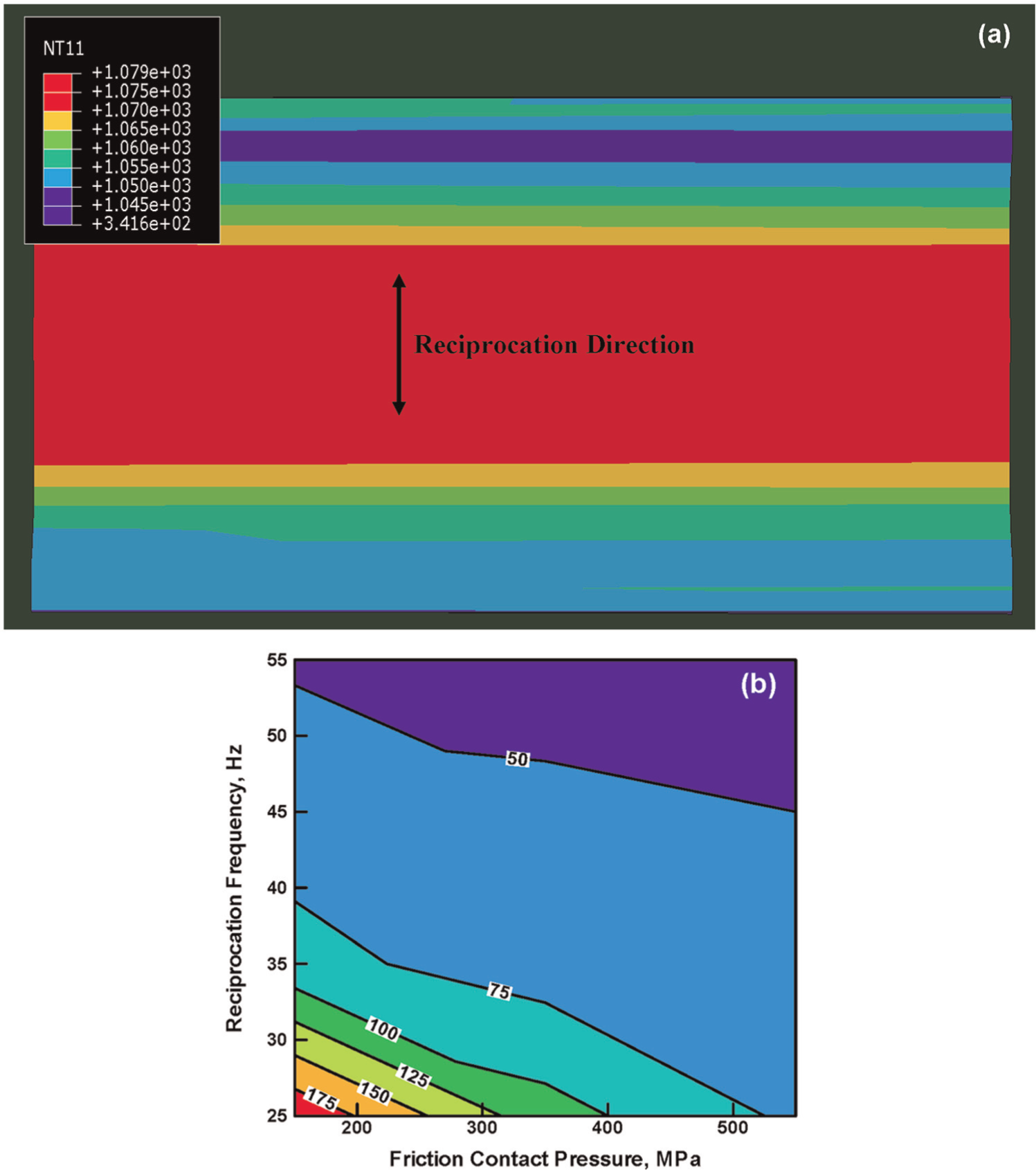
In addition to the spatial distribution of temperature, temporal evolution of the same quantity is of major concern. An example of the typical results pertaining to temporal evolution of temperature at the center of the contact interface is shown in Figure 8(a). It is seen that during the transition phase, temperature steeply rises and that during the equilibrium phase, temperature oscillates over a relatively narrow range. Furthermore, examination of Figure 8(a) suggests that there is a possibility, under the LFW process parameters employed, for formation of austenite at this location (the location which experiences the highest temperatures in the course of LFW), since the maximum temperature (ca 1100 K) exceeds the AS temperature. Clearly, this problem could be overcome by proper selection of the LFW process parameters. In addition, one must take into account the fact that the material residing at the contact interface, that is, the material that is subjected to the highest temperatures, is continuously expelled outward to form flash. Thus, formation of austenite at the contact interface may be considered as of less concern during the LFW process. However, the more definite answer to this question will be provided in the next section where the results yielded by the newly developed LFW microstructure-evolution model will be presented and discussed.
(a) Typical temporal evolution of temperature at the contact interface center point during LFW process simulation of Carpenter Custom 465, H1000, and (b) typical temporal evolution of temperature at five material points within one of the Carpenter Custom 465 workpieces being linear friction welded. Initial distances of the material points from the weld line/interface are denoted in the figure.
Typical results pertaining to the temporal evolution of temperature for five material points within one of the workpieces being linear friction welded are shown in Figure 8(b). Initial distances of the points from the weld line/interface are denoted in the figure. Examination of the results displayed in this figure reveals the expected qualitative behavior of the temperature history as a function of the initial distance of the material point from the weld interface. That is, the closer is the point to the interface, the shorter is the time it takes the heat wave to reach it and the higher is the maximum temperature experienced by the point. In addition, as the time increases beyond the forge step, and the workpiece continues to cool down, temperature differences between different points continuously decrease.
Temporal evolution and geometry of the expelled material/flash
As mentioned earlier, LFW is accompanied by the formation of flash. Flash contains the material that was previously located at the contact surfaces. This material was, in the course of LFW, heated, softened, and subsequently expelled from the contact interface in the direction of reciprocation. The formation of the flash during LFW is highly critical since the expelled material was, before expulsion, typically oxidized, contaminated, or otherwise compromised and its removal creates clean, virgin-material surfaces with high affinity for adhesion/bonding.
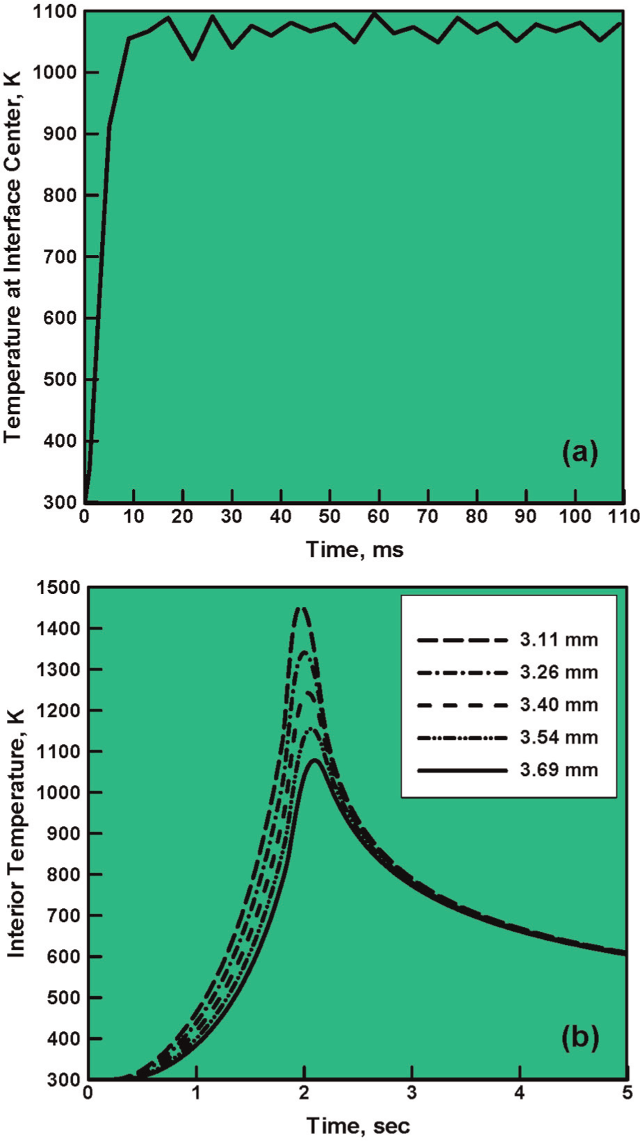
An example of the typical results pertaining to the temporal evolution of flash during the equilibrium phase of LFW of Carpenter Custom 465, H1000, is displayed in Figure 9(a)–(d). It should be noted that a surface temperature contour plot is superimposed onto the material distribution plot in this figure in order to help relate the local temperature with the extent/rate of flash formation. Examination of the results displayed in Figure 9(a)–(d) shows that a single flash (on each weldment side) is formed, suggesting that under the LFW process parameters employed, a good-quality/defect-free weld should be expected.
Typical results pertaining to the temporal evolution of flash during equilibrium phase of LFW of Carpenter Custom 465, H1000. Relative elapsed time: (a) 0 s; (b) 0.12 s; (c) 0.24 s; and (d) 0.36 s. Please note that a surface temperature contour plot is superimposed onto the material distribution plot in order to help relate the local temperature to the extent/rate of flash formation
Temporal evolution of the axial shortening
As the thermally softened interface material is expelled, the height/thickness of the two workpieces being welded is reduced. This phenomenon is commonly referred to as axial shortening and is quantified by the so-called burn-off distance. It is generally accepted that a minimum value of the burn-off distance (which ensures complete removal of the oxidized, contaminated, or otherwise compromised material from the contact surfaces) is necessary for the attainment of a sound weld with good mechanical properties. It is equally well recognized that excessive axial shortening leads to a loss of material and productivity, as well as to an increased cost associated with removal and handling of excessive flash.
An example of typical results pertaining to the temporal evolution of the burn-off distance during LFW of Carpenter Custom 465, H1000, is displayed in Figure 10(a). For improved clarity, different LFW phases are denoted in this figure. It is seen that shortening begins in the initial phase (due to application of the initial contact pressure) and, after a short transition phase, continues throughout the equilibrium phase at a fairly constant average rate. In the forging phase, application of a higher upset contact pressure causes an abrupt jump in the axial shortening.
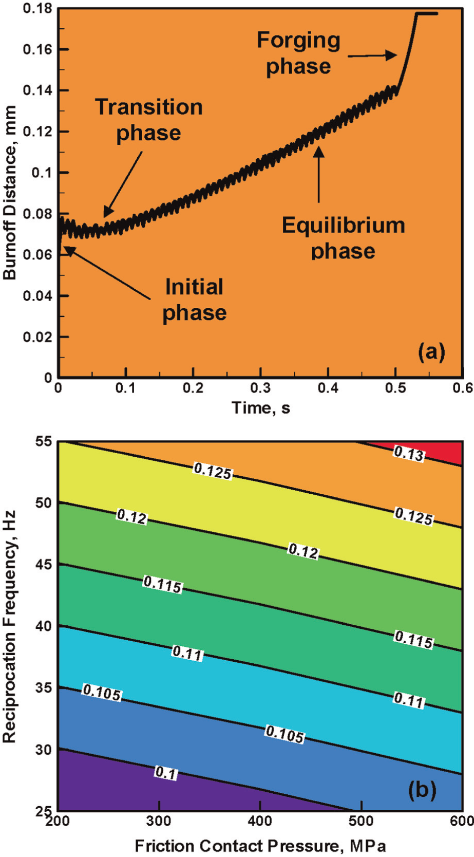
Typical results pertaining to (a) temporal evolution of axial shortening/burn-off distance and (b) the effect of the equilibrium-phase contact pressure and reciprocation frequency, at a constant level of the reciprocation amplitude of 2 mm, on the rate of axial shortening, both for Carpenter Custom 465, H1000.
The average slope of the burn-off distance versus time curve in the LFW equilibrium phase defines the equilibrium rate of axial shortening, also sometimes referred to as the burn-off rate. This quantity plays an important role in the LFW process, since it is generally believed that its value must also exceed a minimum critical level for the attainment of a sound weld.
The burn-off rate is a function of the LFW process parameters. This is demonstrated in Figure 10(b) in which, at a constant level of reciprocation amplitude of 2 mm, a contour plot is displayed showing the effect of the friction contact pressure and the reciprocation frequency on the equilibrium-phase axial-shortening rate. Examination of the results displayed in this figure reveals that as expected, both increases in the friction contact pressure and reciprocation frequency lead to increases in the burn-off rate.
Microstructure evolution in Carpenter Custom 465 during LFW
In this section, the results yielded by the LFW precipitate-evolution model are presented and discussed. The first set of these results deals with the isothermal-aging process, which is used to produce various grades of Carpenter Custom 465 such as H1000 and H950.38–41 The next set of the results reveals typical spatial distribution of the precipitate volume fraction and mean particle size throughout the weld region. 42 The last set of results shows how the choice of the LFW process parameters such as the friction contact pressure and the reciprocation frequency affects the characteristic precipitate size and volume fraction at the contact interface/weld surface. 43
Isothermal aging of Carpenter Custom 465
The results presented in Figure 11(a) and (b) show the effect of the (constant) aging temperature and time on the precipitate mean radius and its volume fraction, respectively. The combination of the aging temperature and the aging time corresponding to Carpenter Custom 465 H1000 is denoted by a black-filled circle. As mentioned earlier, Carpenter Custom in this aged condition is assumed to be used in the LFW process analyzed in this work. Thus, the values of the mean particle radius (~0.474 µm) and the precipitate volume fraction (~0.0694) define the state of the aging/precipitation found in the as-received condition of Carpenter Custom 465 H1000.
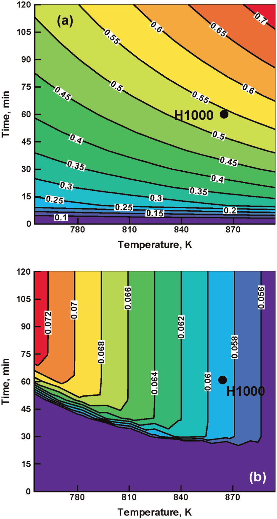
Effect of aging temperature (K) and the aging time (min) on the precipitate: (a) mean radius and (b) volume fraction in Carpenter Custom 465. Black-filled circle is used to denote the H1000-aged condition analyzed in this work.
Examination of the results displayed in Figure 11(a) and (b) reveals the following:
As the aging temperature increases, at a constant aging time of 60 min, the precipitate mean radius increases. This observation is evidence of the operation of the precipitate-coarsening processes.
As the aging temperature increases, at a constant aging time of 60 min, the precipitate volume fraction decreases. This result is a consequence of the fact that the solubility of the alloying elements increases, and consequently, the equilibrium volume fraction of the precipitates decreases, with an increase in temperature.
Effect of LFW on Carpenter Custom 465 weld microstructure
It should first be noted that the results presented and discussed in this section are obtained under the same LFW process parameters as those specified in section “Typical results yielded by the LFW thermo-mechanical process model.” The corresponding results, but under different LFW process conditions, were also generated within this work. However, they are not shown for brevity. On the other hand, some aspects of these additional results will be presented in the next section.
Figure 12(a)–(d) shows spatial distribution of the precipitate mean radius over the x–y section at four distances (0.0, 1.0, 2.0, and 3.0 mm) from the contact interface. It should be noted that material residing within the flash is not accounted for in these figures, as well as in the subsequent figures, for the following two reasons: (a) this material does not ultimately reside within the weldment and, hence, its precipitate microstructure is of no concern and (b) the material residing within the flash is typically subjected to excessive temperatures, which may result in martensite → austenite reversion, the phase transformation that was not analyzed in this work. Nevertheless, it should be noted that microstructural examination of the material residing within the flash can provide important data, which could be used to validate a microstructure-evolution model (once consideration is given to the martensite → austenite reversion).
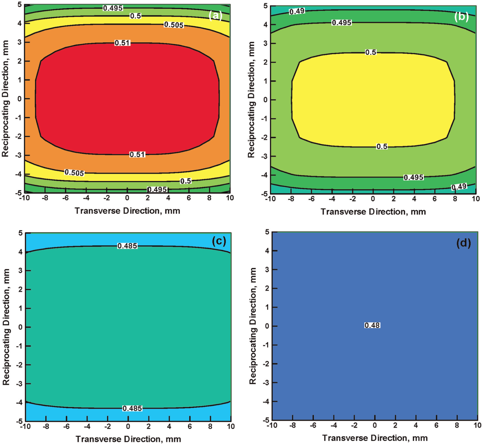
Spatial distribution of the precipitate mean radius µm), over the x–y sections located at distances of (a) 0.0 mm, (b) 1.0 mm, (c) 2.0 mm, and (d) 3.0 mm from the contact interface, in LFWed Carpenter Custom 465, H1000. Please see text for details of the LFW process parameters used.
Examination of the results displayed in Figure 12(a)–(d) reveals the following: (a) precipitate size is generally non-uniform over a given x–y section; (b) the extent of particle size non-uniformity decreases with an increase in distance from the contact interface and effectively vanishes at a distance greater than 3.0 mm; (c) at the contact interface, the largest precipitate sizes are found in the innermost portion of the corresponding x–y section, the portion that experiences the highest temperature. The edge portions of this section contain smaller particle sizes due to the operation of heat-transfer processes between the workpieces being welded and the surroundings; (d) the precipitate mean radius decreases with distance from the contact interface, showing that the largest precipitate-coarsening effects are found at the contact interface itself; (e) precipitate-coarsening effects are seen at the largest distance analyzed, 3.0 mm from the interface (Figure 12(d)); and (f) some evidence of precipitate coarsening is obtained even at distances of 5.0–6.0 mm from the interface (the results are not shown for brevity).
Figure 13(a)–(d) shows spatial distribution of the precipitate volume fraction over the x–y section at four distances (0.0, 1.0, 2.0, and 3.0 mm) from the contact interface. Examination of the results displayed in these figures reveals the following:
Precipitate volume fraction is generally non-uniform over a given x–y section.
The extent of precipitate volume fraction non-uniformity decreases with distance from the contact interface and effectively vanishes at a distance greater than 2.0 mm.
The smallest values of the precipitate volume fraction are found in the innermost portion of the corresponding x–y section, the portion that experiences the highest temperature. The precipitate volume fractions found in this portion of the contact interface are smaller than their counterparts found in the as-received Carpenter Custom 465 H1000, revealing the operation of precipitate-dissolution processes. Precipitate volume fractions in the edge portions of the contact interface section are somewhat higher, suggesting a lower extent of particle dissolution. This finding is consistent with the aforementioned thermal effects related to heat-exchange processes between the workpieces being welded and the surroundings.
As the distance from the interface increases, the extent of precipitate dissolution decreases and ultimately ceases. Meanwhile, resumption of precipitate formation takes place, causing an increase in the precipitate volume fraction (at distances greater than or equal to 2.0 mm) (Figure 13(c)).
The extent of increase in the precipitate volume fraction gradually decreases with an increase in the distance from the contact interface.
At distances of approximately 5.0 mm from the contact interface, no evidence of measurable change in the precipitate volume fraction relative to that found in the as-received Carpenter Custom 465 H1000 could be found (the results are not shown for brevity).
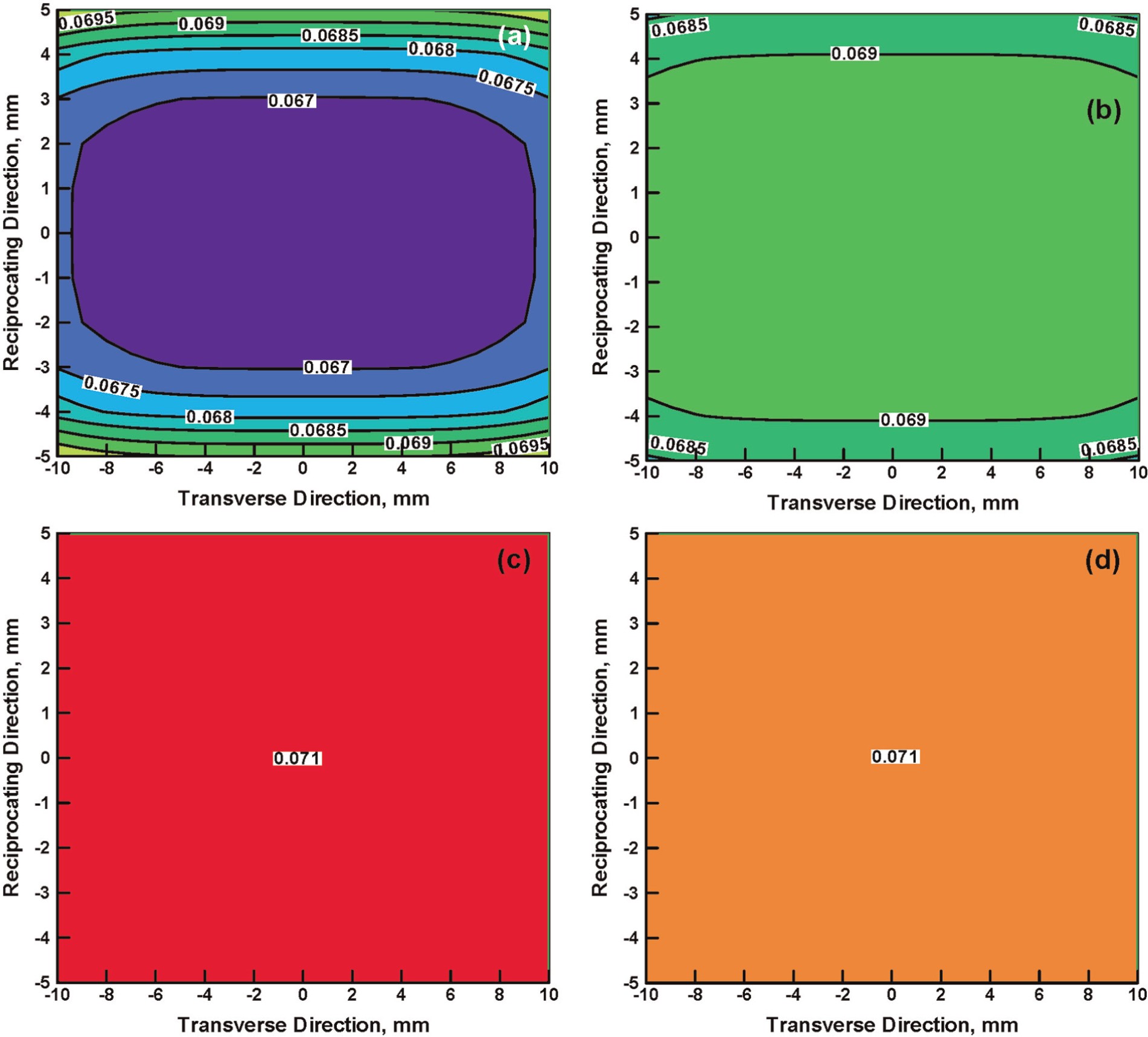
Spatial distribution of the precipitate volume fraction, over the x–y sections located at distances of (a) 0.0 mm, (b) 1.0 mm, (c) 2.0 mm, and (d) 3.0 mm from the contact interface, in LFWed Carpenter Custom 465, H1000. Please see text for details of the LFW process parameters used.
Effect of LFW process parameters on weld microstructure
As mentioned earlier, combined application of the LFW process model and the LFW weld microstructure-evolution model can be used to establish relationships between the LFW process parameters, on one hand, and the weld microstructure (and its spatial distribution), on the other hand. These relationships, in turn, can be used to identify optimal LFW process parameters. In this section, a couple of prototypical results are shown, which demonstrate the relationship between the LFW process parameters and the weld microstructure.
The effect of the (equilibrium-phase) friction contact pressure (in the 100–500 MPa range) and the reciprocating frequency (in the 30–70 Hz range) on the precipitate mean radius (µm) and the precipitate volume fraction, at the mid-point (x = y = 0.0) of the contact interface in Carpenter Custom 465, H1000, is shown in Figure 14(a) and (b), respectively. The remaining LFW process parameters are identical to the ones specified earlier in Section “Typical results yielded by the LFW thermo-mechanical process model.” A black-filled circle is used in Figure 14(a) and (b) to denote the baseline LFW process parameters that were employed in the computational analysis that yielded Figures 12 and 13 (i.e. friction contact pressure = 150 MPa, reciprocation frequency = 50 Hz).
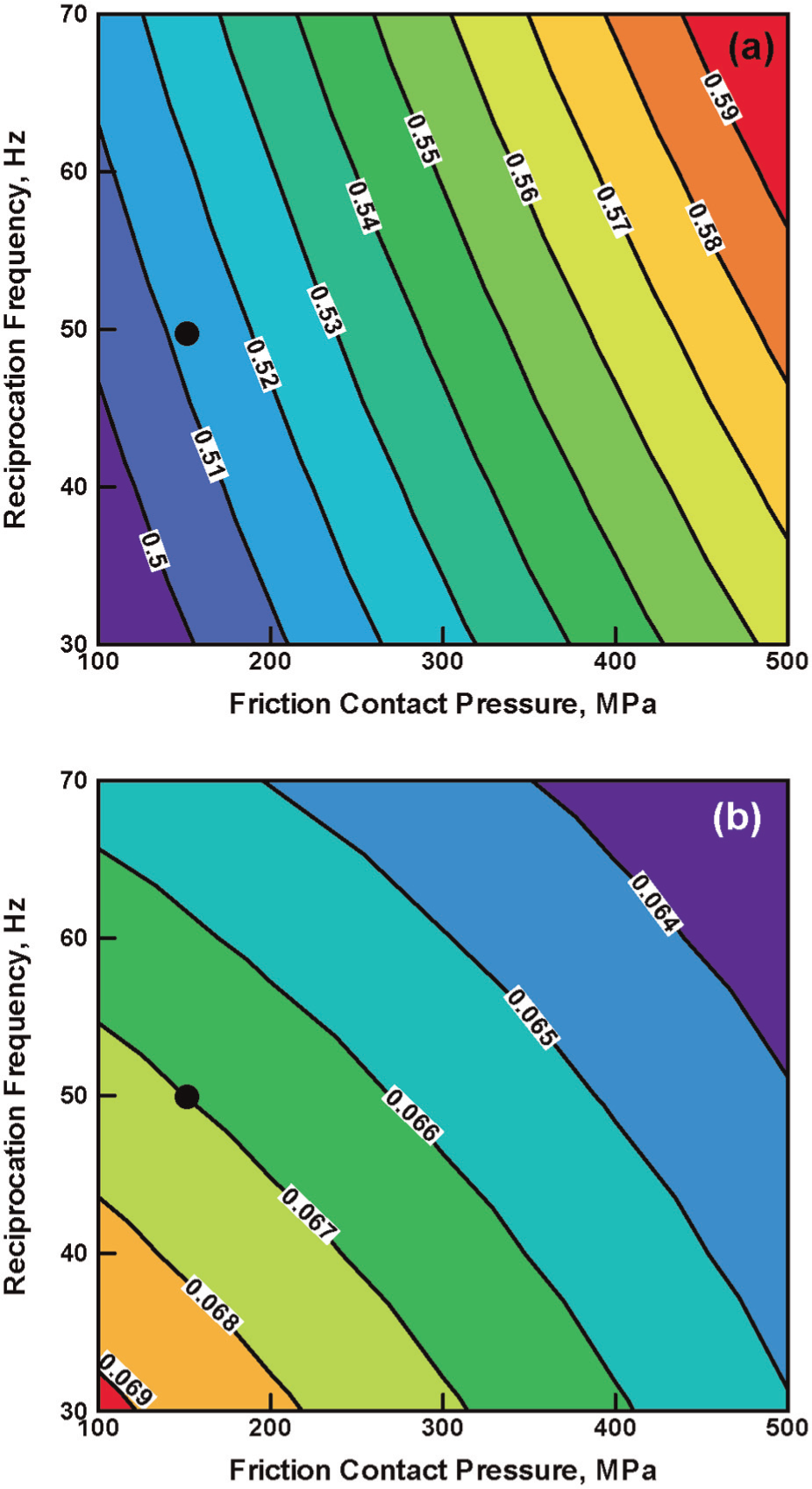
Effect of the (equilibrium-phase) friction contact pressure and reciprocation frequency on the precipitate: (a) mean radius (µm) and (b) volume fraction, at the center point (x = y = 0) of the contact interface, in Carpenter Custom 465, H1000. Please see text for details of the remaining LFW process parameters used. Black-filled circle denotes the baseline LFW process parameters that were employed in the computational analysis that yielded Figures 12 and 13.
Examination of Figure 14(a) shows that the largest precipitates are found in the LFW weld obtained under the combination of the largest friction contact pressure and the highest reciprocation frequency. This finding is fully expected since these LFW process conditions yield the highest temperature at the contact interface and, hence, give rise to the largest extent of precipitate coarsening.
Examination of the results displayed in Figure 14(b) reveals the following:
As the friction contact pressure and the reciprocating frequency increase, the precipitate volume fraction decreases. Consequently, the lowest value of the precipitate volume fraction is found for the LFW process conditions corresponding to the largest value of the friction contact pressure and the highest value of the reciprocating frequency.
Depending on the LFW process conditions, precipitate volume fractions could become either higher or lower than their counterpart in the as-received Carpenter Custom 465, H1000, condition. This finding suggests that depending on the LFW process condition selected, either precipitate dissolution or precipitate-formation process may prevail.
Jointly, the results displayed in Figure 14(a) and (b) show that LFW process conditions associated with large friction contact pressure and high reciprocation frequencies may result in undesirable LFW weld microstructure, that is, microstructure that is characterized by a smaller volume fraction of coarser precipitates. It should be noted that at a fixed volume fraction of precipitates, the precipitate size scales inversely with precipitate number density. Thus, at the highest levels of the friction contact pressure and reciprocation frequency, the LFW weld microstructure is characterized by precipitates that have the smallest volume fraction and the smallest number density. This combination of the precipitate volume fraction and number density is undesirable since the material strength scales with these two precipitate-microstructure parameters.
The analysis presented above clearly demonstrates the established functional relationships between the LFW process parameters and the resulting weld microstructure properties. These functional relationships can be used to tailor/set up the LFW process in order to minimize the extent of material microstructure/property degradation within the weld. However, additional aspects of the LFW process such as weld integrity, energy efficiency, and process throughput must also be addressed. This requires the use of a constrained multi-objective optimization scheme. Within such a scheme, optimal LFW process parameters will be identified which both satisfy the imposed constraints (e.g. those related to the minimum power input, or minimum burn-off rate) and maximizes the attainment of the conflicting objectives (e.g. minimize microstructure/property degradation, maximize power efficiency, and maximize process throughput). Development of such an optimization scheme is beyond the scope of this work, but is the subject of our ongoing work. The preliminary results suggest that one can ensure minimal losses in the weld microstructure properties without significant sacrifice in the process throughput.
Summary and conclusion
Based on the work presented and discussed in this article, the following main summary remarks and conclusions can be made:
A new LFW microstructure-evolution model has been developed in order to predict the type, the extent, and the temporal evolution and spatial distribution of microstructural changes within different portions of the weld. The newly constructed LFW microstructure-evolution model includes the main physical metallurgy concepts and principles of the workpiece material and accounts for the basic thermodynamics and kinetics of various interacting and competing phase transformations, which may take place within the weld region.
The LFW microstructure-evolution model is subsequently combined with our recently developed fully coupled thermo-mechanical finite element–based LFW process model and applied to Carpenter Custom 465, H1000, a high-strength/high-corrosion resistance, PH martensitic stainless steel.
Combined use of the LFW process and microstructure-evolution models enabled establishment of the basic functional relationships between the LFW process parameters (e.g. friction pressure, reciprocating amplitude, reciprocating frequency, and forging pressure) and the spatial distribution of the precipitate microstructure within the weld region.
It is shown that these functional relationships can be used to tailor/set up the LFW process in order to minimize the extent of material microstructure/property degradation within the weld, without seriously compromising energy efficiency or throughput of the process.
Footnotes
Acknowledgements
The authors are indebted to Dr Ralph A. Anthenien Jr of ARO for his continuing support and interest in this work. The authors would also like to thank Dr David Bowden for helpful discussions and encouragement.
Declaration of conflicting interests
The authors declare that there is no conflict of interest.
Funding
The initial portion of the work presented in this article was supported by the Army Research Office (ARO) through the grant Friction Stir Welding Behavior of Selected 2000-series and 5000-series Aluminum Alloys, Project No. W911NF-11-1-0207.