Sage Journals: Discover world-class research

Abstract

The feature selection function in data mining facilitates the classification of vast data volumes and reduces attribute variables, enabling the construction of classification prediction models. For binary data, the Mahalanobis–Taguchi system, the logistic regression method, and the neural network method all feature high stability and accuracy. The Mahalanobis–Taguchi system differs from the other two methods in that models are developed through a measurement scale rather than from the learning of analytical data. We analyzed the audit quality of Taipei City Government public procurement from supply chains (hereafter abbreviated as public procurement) and applied the three feature selection methods to determine the items used in public procurement audit quality questionnaires. The results showed that the predictive powers of Mahalanobis–Taguchi system and logistic regression methods for the reduced question items were 93.8% and 92.5%, respectively. Furthermore, the prediction accuracy rate of the neural network method was 100%, showing that the prediction model constructed using the feature selections to reduce the number of attributes can effectively lower the number of questionnaire items while maintaining high prediction accuracy.

Keywords

Feature selection data mining Mahalanobis–Taguchi system logistic regression neural networks procurement

Introduction

In recent years, enhanced access to information has rendered data access much easier than it has been in the past. However, to acquire useful information from a sea of data or to use data to build a prediction model, data mining technology must be employed. One of the major processes in data mining is classification; to improve the efficiency of classification, feature selection is generally used for constructing classification models. For binary classification, the ratio among the various data classes used for analysis is a key factor influencing classifier learning.^1–5 By adopting diversified feature selection methods, we can reduce feature numbers and increase accuracy rates, ultimately producing a variety of classification models. To ensure the classification quality, most classification models conduct data feature selection to prevent redundant or unrelated features from affecting classification accuracy.⁶

The Mahalanobis–Taguchi system (MTS), which was first proposed by Dr Genichi Taguchi, includes principles and advantages of mathematics, statistics, and robust design and can be used to perform multivariate analyses and predict and select crucial attribute variables. MTS employs the Mahalanobis distance (MD), which is based on correlations between variables, as a measurement scale for multivariate systems and performs system optimization based on robust design principles. In practice, MTS has been successfully and extensively applied in disease diagnosis, earthquake prediction, individual credit evaluation, and voice identification or recognition.^7–9 Moreover, MTS, logistic regression, and neural networks all demonstrate excellent discrimination in solving binary classification problems using multivariate data. All the three models can be used to classify imbalanced binary classification data. The prediction models were developed by reducing attribute variables. Therefore, this study adopts the MTS, logistic regression, and neural networks in designing audit quality questionnaires for government procurement agencies and establishes a reduced questionnaire model that possesses high precision and reliability.

Moreover, procurement staffs from various units of the Taipei City Government were used as an example. Units demonstrating superior government procurement audit quality were considered normal samples and adopted as the basis for variable reduction. Units possessing poor audit quality were regarded as abnormal samples and used to verify whether the reduced variables demonstrated appropriate differentiability.

Literature review

MTS

The MTS is a new classification technology presented by Dr Genichi Taguchi for conducting diagnosis and forecasting using multivariate data. It combines quality engineering principles and the MD for the structured induction of data, which serves as a basis for decision making.^10–12

MD

MD, introduced in 1939 by an Indian statistician, PC Mahalanobis, is a type of statistical distance that accounts for the relationship between attribute variables. Compared to the Euclidean distance (ED), MD incorporates correlations among variables into consideration, despite the fact that both MD and ED measure the distance between unknown sample points and reference populations. Figure 1 presents the difference between MD and ED.

Figure 1.

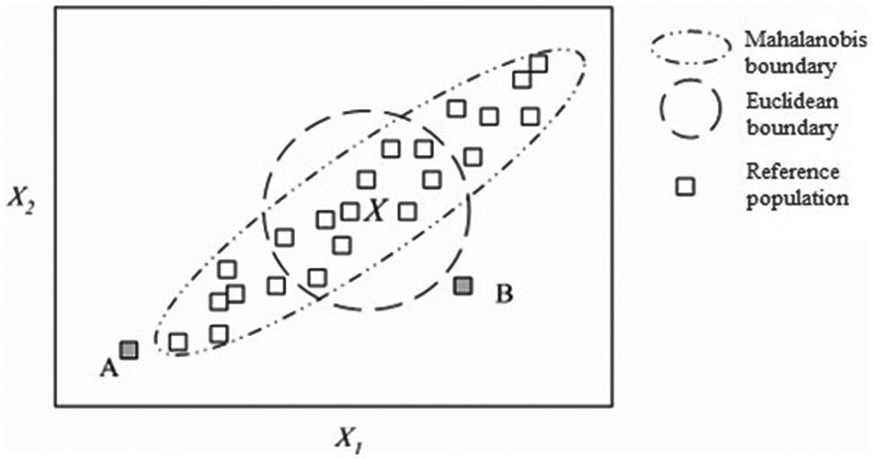
Difference between MD and ED.

Orthogonal array

In robust designing, the purpose of using orthogonal arrays (OAs) is to minimize the number of experiments required to achieve a more reliable estimation regarding factor effects. In MTS, an OA identifies useful and applicable variables with a minimum number of experiments. Variables are allocated to different columns in an OA, and each variable possesses two levels: Level 1 in the OA indicates that the variable is used to calculate MD, whereas level 2 implies that the variable is not used to calculate MD.

Signal-to-noise ratio

In quality engineering, signal-to-noise (S/N) ratio is an assessment tool that is expressed in decibels. S/N ratio evaluates functions or performances using the ratio of useful information to false or irrelevant data. For multivariate data, a set of variables that can accurately detect the degree of abnormality is extremely crucial. Regarding the MTS, Dr Taguchi proposed two methods to calculate S/N ratios: (a) the larger-the-better S/N ratio and (b) dynamic S/N ratio. Because the degree of abnormality was required to be measured for two questionnaires and used as basis for screening or selecting variables and because that MDs in abnormal observations were expected to be greater than those in normal observations, the larger-the-better S/N ratio was used in this study.

Logistic regression

Logistic regression was developed by Berkson¹³ and is used to resolve the problem that test results can only produce binary data (e.g. success or failure). In the process of establishing a model, Berkson endeavored to accurately predict the relationship between response variables and a set of independent explanatory variables. He established a set of classification rules by which the probability of success can be predicted through a single sample to ultimately determine the attribute of the sample. Logistic regression is a statistical analysis for processing categorical dependent variables and is primarily adopted in solving classification problems. The final predicted value is a probability ranging from 0 to 1.¹⁴ Following the development of the logistic regression, Srinivisan¹⁵ was the first to employ this analysis and allocated scores according to variable weights. In contrast to linear discriminant analysis, logistic regression does not require pre-assumptions. Harrell and Lee¹⁶ found that the logistic regression model achieves better accuracy compared to the linear discriminant analysis. Thus, logistic regression has been widely applied in social studies, bankruptcy prediction, market segmentation, customer behavior, and the establishment of classification models for personal loans.^17,18 Tam and Kiang¹⁹ and Zhang²⁰ focused on bankruptcy and conducted classification prediction using classification methods such as logistic regression, neural networks, linear discriminant analysis, and decision trees for comparisons.

Neural networks

The neural network was first proposed in 1890 and is a type of algorithm that was established to imitate the manner in which human brains process information. Subsequently, McCulloch and Pitts²¹ developed a mathematical model for neurons. Rosenblatt²² established the perceptron, which repeatedly adjusts weights to enhance learning abilities satisfactorily. Neural networks became popular between 1957 and 1969; however, because computers at that time were insufficient in computing power, their learning abilities were restricted, and neural network ceased to be popular for a period of time. It was only in 1985 when new computation methods were developed that the neural network became widely used again.^23,24

The algorithm for neural networks involves the adoption of mathematical languages to describe the operation model of the human brain, which is referred to as a neural network. Neural networks are characterized by the ability of self-learning. Instead of designing complicated programs, users can resolve problems simply by providing data, from which neural networks can learn.²⁵ Neural networks have been extensively used in industrial control, business decision making, stock and exchange rate prediction, voice identification systems, and fault-tolerant systems.²⁶ A neural network is composed of neurons, including input and output neural nodes, as shown in Figure 2. The central section is a layer of invisible hidden nodes and can be regarded as a black box. Hidden nodes are responsible for complex computations. Because the means by which results are generated is unknown, only input and desired output are required once the neural network model that will be used to resolve problems is determined. Neural network models can be utilized instantly after training without having to determine the connected weights of internal nodes.^24,27–30

Figure 2.

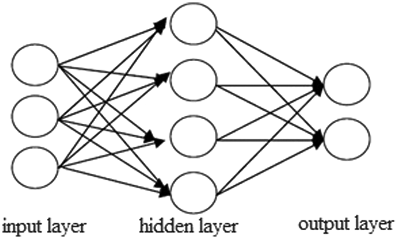
A neural network.

Research and analysis

Public procurement from supply chains, also known as unified or public procurement, is the behavior of government agencies to satisfy the needs of public services by procuring or purchasing goods, engineering projects, and services from international and domestic markets through legal means, methods, and procedures under financial supervision. Government procurement not only entails a specific procurement process but also encompasses procurement policies, procedures, and management. The major problems involved in government procurement include consensus or mutual understanding among procurement units (legal and practical experiences), transparency of government procurement procedures and procurement efficiency, and monitoring and supervision of performances (auditing system and indicators). From a government perspective, the main concern is quality control (i.e. selection criteria and approaches for construction tendering or bidding in government procurement), and from the perspective of tendering vendors, risk assessment should be the focus (i.e. investment costs, implementation ability, which includes the ability to resolve subcontracting problems, and risks related to natural disasters). Thus, methods to implement win-win decision makings and ensure that procurement staffs of government agencies do not violate regulations stipulated in the Government Procurement Act must be based on public interest, procurement efficiency, and professional judgment to generate appropriate procurement decisions. Consequently, to accurately measure the audit quality of government procurement, a systematic approach is required for developing suitable audit quality scales.

MTS analysis

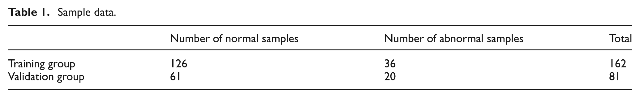
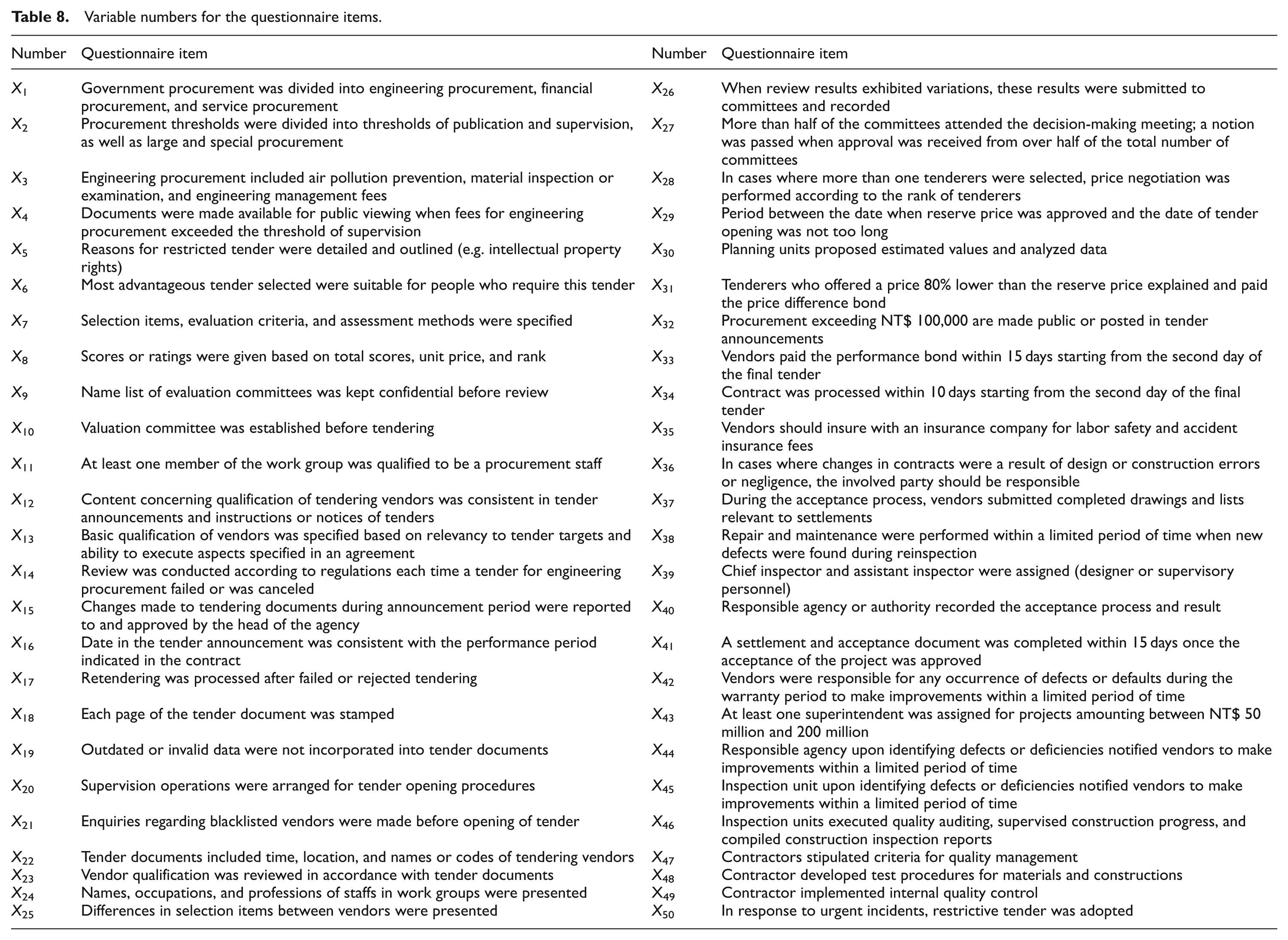
To facilitate efficient calculation using MTS, the 50 items in the questionnaire were each allocated a variable number (X₁ to X₅₀) (please refer to Appendix 1). This article used MATLAB program to calculate the MTS. Subsequently, a total of 243 valid questionnaires were obtained as sample data, of which 162 were categorized as the training group, which included 126 normal data samples and 36 abnormal data samples. Among the samples, 81 were adopted as the validation group to validate the model. The number of collected sample data is presented in Table 1. The 126 normal samples in the training group were adopted as the basis to establish the Mahalanobis space (MS), which included population average values, standard deviations (SDs), and inverse correlation matrices.

Table 1.

Sample data.

	Number of normal samples	Number of abnormal samples	Total
Training group	126	36	162
Validation group	61	20	81

After obtaining the MDs for the training group, a frequency distribution chart was compiled, as shown in Figure 3. The result shows that the majority of MDs for the abnormal samples were larger than those for the normal samples. Moreover, under a threshold value of 2.0, the accuracy rate reached 91.3%. Therefore, the MS was a satisfactory inters of scale.

Figure 3.

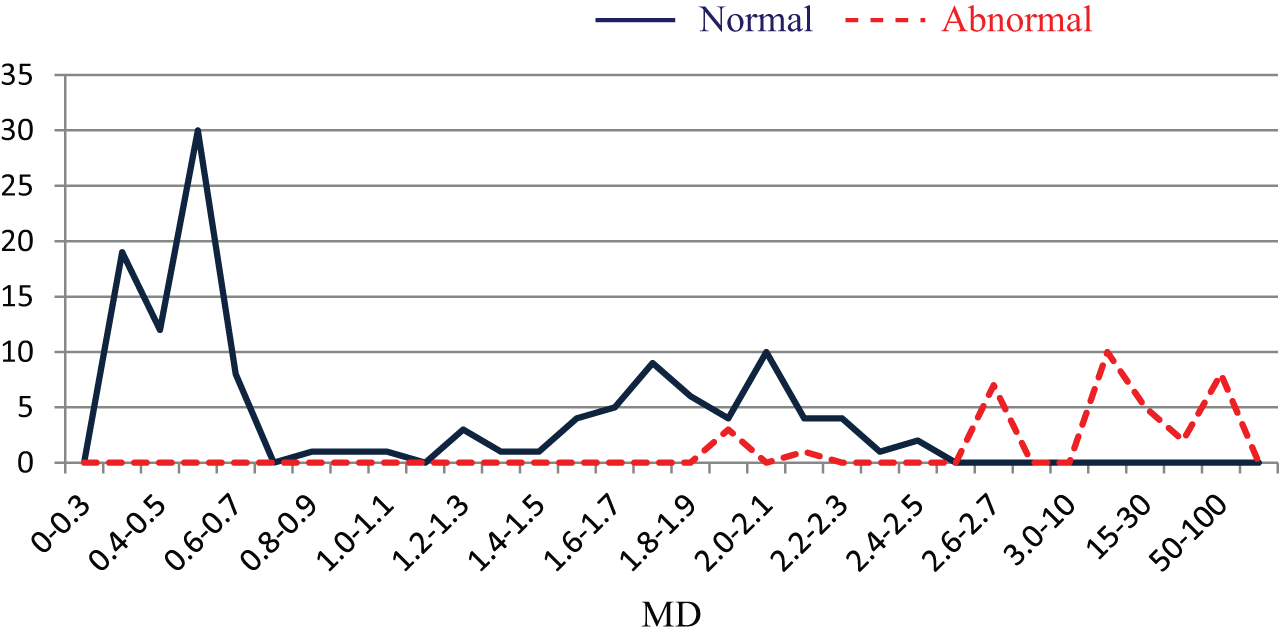
Distribution diagram of the MDs for the training group (k = 50).

The MS established using the training group data was used to calculate the MDs for the normal and abnormal samples of the validation group. The results were then compiled into a frequency distribution chart, as shown in Figure 4. The MDs for the abnormal samples were substantially larger than those for the normal samples. Similarly, an accuracy rate of 98.7% was achieved when the threshold value was set to 2.0. The results indicate that the measurement scale developed using 50 variables is superior and effective. Thus, in the next section, this study investigated whether the number of variables and items could be reduced to still obtain satisfactory accuracy.

Figure 4.

Distribution diagram of the MDs for the validation group (k = 50).

To select crucial variables and eliminate irrelevant variables from the questionnaire, an OA was used to determine the effects that each questionnaire item has on analysis results following the procedure below: (a) the variables were divided into two levels, where Level 1 indicated that the variable should be used and Level 2 implied that the variable should not be used. (b) These variables were then arranged into the OA. This study adopted 50 variables; thus, the L₆₄ (2⁶³) OA was utilized. (c) The 36 abnormal samples in the training group were used to calculate the 36 corresponding MDs, and the S/N ratio recommended by Taguchi (the larger-the-better type) was employed. The larger-the-better principle for S/N ratios also applies to the gains of variables. In other words, larger gains indicate that better results can be generated. Figure 5 shows the gains of variables.

Figure 5.

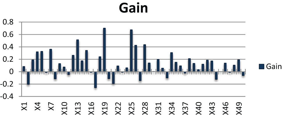
Gain of variables.

The differences in variable gain are shown in Figure 3. By selecting based on differing gain values (>0, >0.1, >0.2, >0.3, >0.4), the number of questionnaire items (originally 50) was reduced to 34, 26, 13, 10, and 5, respectively. Subsequently, a model with a reduced number of variables was obtained, and the final characteristics were selected according to the group (training or validation group) that had the higher accuracy rate, as shown in Table 2.

Table 2.

Comparison of the effects of differing variable gain values.

Gain	Questionnaire item	Threshold value	Training group	Validation group
>0	34	1.9	88.9%	92.6%
>0.1	26	2.1	90.1%	93.8%
>0.2	13	1.6	87%	93.8%
>0.3	10	2.0	88.3%	83.9%
>0.4	5	2.0	83.3%	87.6%

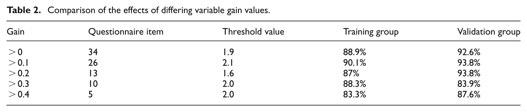
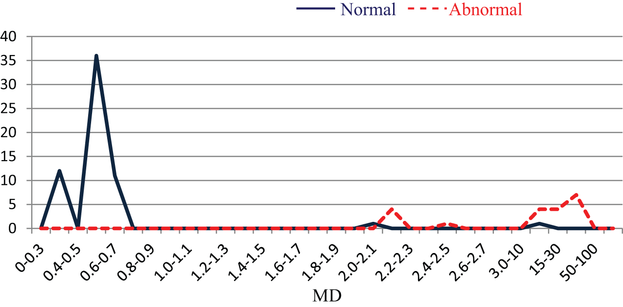
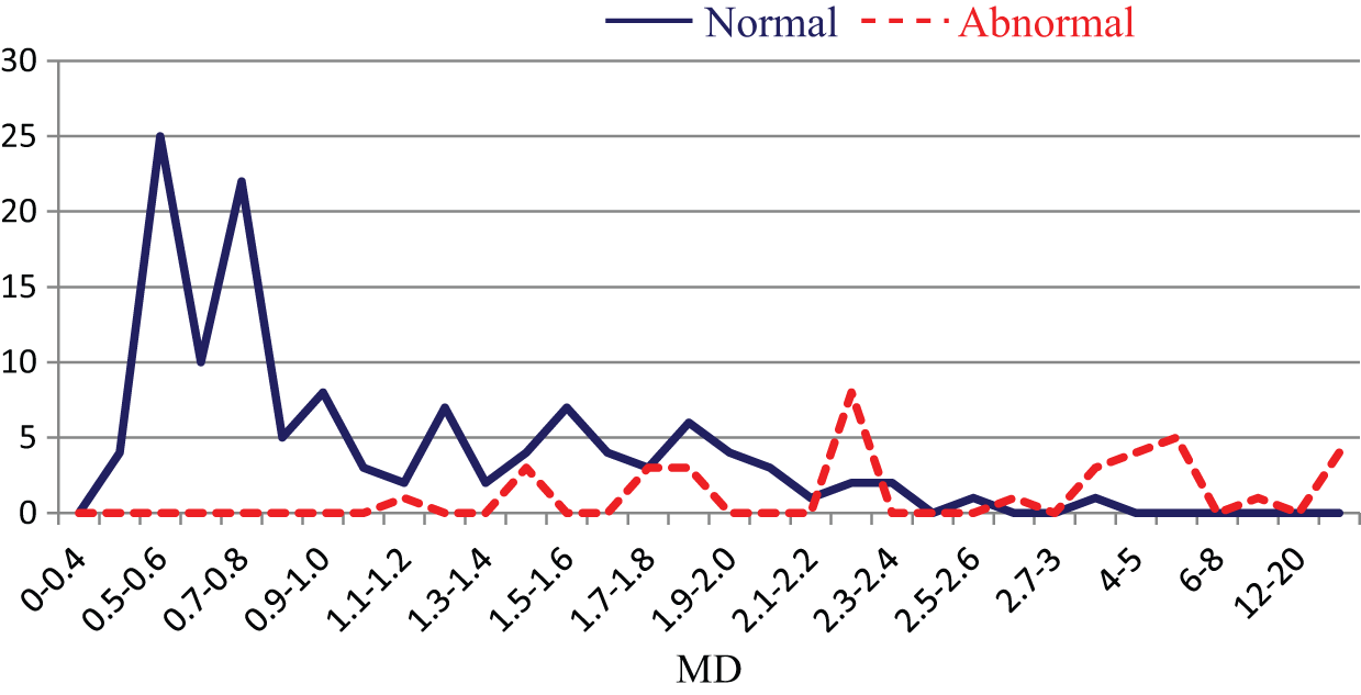
Using gain >0.1 as an example, the number of questionnaire items was reduced from the original 50 to 26, as shown in Table 2. The data of the normal samples in the training group and the selected 26 crucial item variables were used to reconstruct an MS. The abnormal samples were adopted for verifying or validating the scale of the reduced model. Subsequently, a frequency distribution chart was compiled. The minimization of Type I and Type II errors was employed as a reference for determining the threshold value. As shown in Figure 6, at a threshold value of 2.1, the accuracy rate reached 90.1%. The sample data for the validation group were then used to determine whether a similar accuracy rate could be obtained when the number of variables decreased to 26. Similarly, as shown in Figure 7, according to the frequency distribution chart for the validation group, the accuracy rate reached 93.8% at a threshold value of 2.1.

Figure 6.

MD distribution chart for the training group (k = 26).

Figure 7.

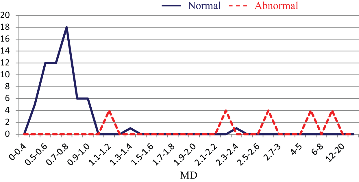
MD distribution chart for the validation group (k = 26).

Therefore, employing the MTS method enabled reducing the items in the government procurement audit quality questionnaire from 50 to 26. Validation results from the various participant groups confirmed that the questionnaire still featured a high accuracy rate, indicating that the MTS is a feasible method for reducing the number of questionnaire items.

Logistic regression analysis

The same set of data used in the previous section was also employed for the logistic regression analysis to establish a model by adopting binary variables (normal samples as 0 and abnormal samples as 1) as the dependent variables and the 50 questionnaire items as the independent variables. Based on the analysis results on variable coefficients using the binary logistic regression function provided by SPSS and MATLAB, numerous variables were not significant; thus, only several attribute variables possessed significant effects on the audit quality scale for government procurement. Hence, the researchers reconsidered using key factors to establish a logistic regression model.

This study adopted the backward stepwise selection method to identify key factors for selecting questionnaire items using logistic regression. All variables were first incorporated into the logistic regression model, and the threshold for selection and elimination was predefined. Subsequently, among the variables that were included in the backward stepwise elimination, the independent variables with the lowest explanatory power were excluded from the model. Concurrently, the researchers determined whether variables that were not initially included in the model were qualified to be selected. The entry stepwise probability was set to 0.05, and the removal stepwise probability was set to 0.1. The stepwise regression analysis selected 18 key influential factors from the original 50 attribute variables. The reduced equation is expressed as

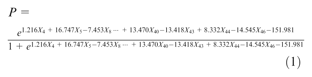
P = \frac{e^{1.216 X_{4} + 16.747 X_{5} - 7.453 X_{8} \dots + 13.470 X_{40} - 13.418 X_{43} + 8.332 X_{44} - 14.545 X_{46} - 151.981}}{1 + e^{1.216 X_{4} + 16.747 X_{5} - 7.453 X_{8} \dots + 13.470 X_{40} - 13.418 X_{43} + 8.332 X_{44} - 14.545 X_{46} - 151.981}}

(1)

Following the attainment of a reduced model, the 162 data entries for the training group (126 normal samples and 36 abnormal samples) were substituted into the model to calculate the probability of an event. Based on different classification cutoff values, Type I error, Type II error, and accuracy rate were calculated. Using minimization of Type I and Type II errors as a reference for determining the threshold value, an accuracy rate of 96.9% was obtained when the cutoff value was set to 0.5. Subsequently, the researchers examined the accuracy rate of the reduced model using the data of the validation group (Table 3). The validation group data included 138 normal samples and 12 abnormal samples, which were then substituted into the reduced equation (equation (1)) obtained using the training group data. The results showed that an accuracy rate of 92.5% was achieved with a cutoff value of 0.5.

Table 3.

Accuracy rate of the logistic regression reduced model.

	Normal (actual)	Abnormal (actual)	Accuracy rate
Training group
Normal	124	2	96.9%
Abnormal	3	33	96.9%
Validation group
Normal	58	3	92.5%
Abnormal	3	17	92.5%

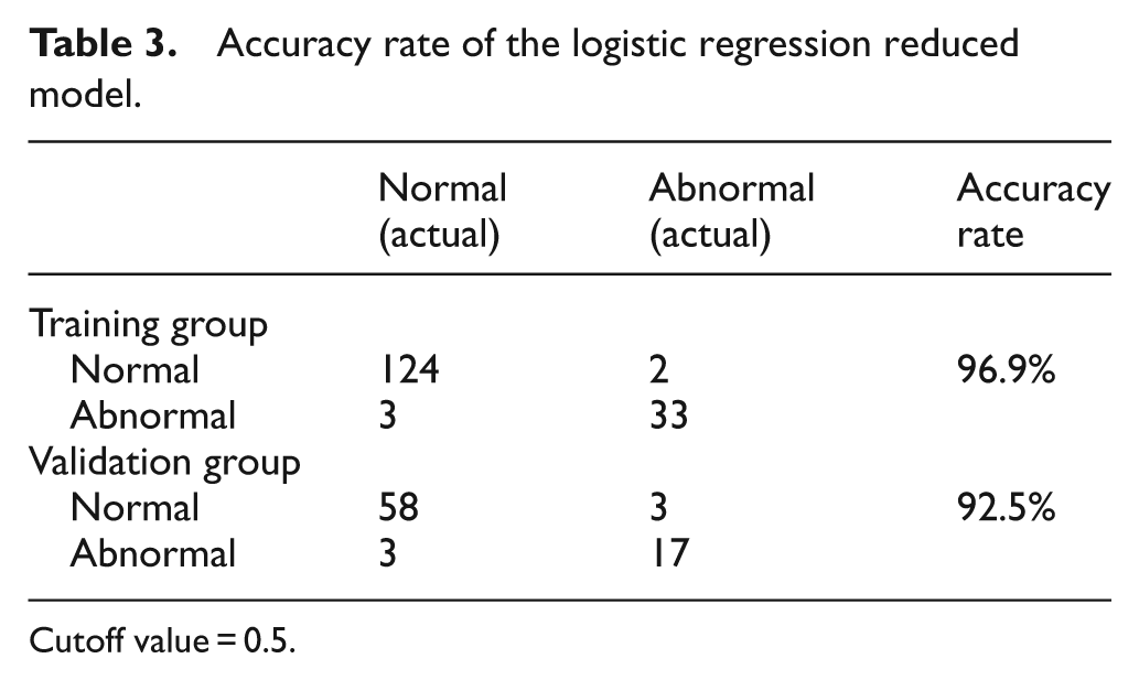
Cutoff value = 0.5.

The logistic regression analysis could reduce the number of items in the quality scale from 50 to 18, and the reduced model was then validated using the validation group sample data. The validation results indicated that an optimal accuracy rate was achieved. Therefore, the adoption of the traditional logistic regression is proved to be applicable to selecting questionnaire items.

Neural network analysis

In this section, the neural network was adopted to identify crucial attribute variables from questionnaire items. The returned 243 data entries were divided into the training group (162) and the validation group (81). The multilayer perceptron (MLP) procedure of neural networks in the SPSS and MATLAB software was employed to develop a prediction model, using the following specifications: (a) 50 nodes in the input layer (i.e. the 50 questionnaire items); (b) one hidden layer, where the hyperbolic tangent function was used as the activation function; and (c) two nodes in the output layer (i.e. the normal and abnormal samples).

Based on the results of the neural network calculation, the accuracy rate for the 162 training group data entries (126 normal and 36 abnormal samples) was 100%, indicating a superior training performance. The importance indicators for test variables are shown in Table 4 . Subsequently, the 81 data entries of the validation group (61 normal samples and 20 abnormal samples) were validated using a trained neural network model. As shown in the prediction table of the neural network analysis, the accuracy was 100%. Therefore, after reducing the number of variables, the researchers further investigated whether an optimal accuracy rate could be attained through the neural network analysis using the quality scale with fewer questionnaire items.

Table 4.

Importance indicators of the independent variables.

Variables	Importance	Normalized importance (cumulative percentage)
X ₁₃	0.050	100.0
X ₂₄	0.042	85.0
X ₁₄	0.035	69.6
X ₃₀	0.034	68.9
X ₃₄	0.034	68.5
X ₁₅	0.033	65.7
X ₂₆	0.032	63.9
X ₂₅	0.029	58.7
X ₄	0.028	57.1
X ₆	0.028	56.9
X ₃₉	0.028	55.5
X ₂₂	0.028	55.5
X ₁	0.027	53.5
X ₁₈	0.026	52.5
X ₄₀	0.026	51.7
X ₂₇	0.024	48.7
X ₉	0.024	48.5
X ₃₈	0.024	47.3
X ₃	0.023	46.3
X ₁₉	0.023	45.4
$⋮$	$⋮$	$⋮$
X ₂₉	0.006	12.6
X ₃₃	0.006	12.0

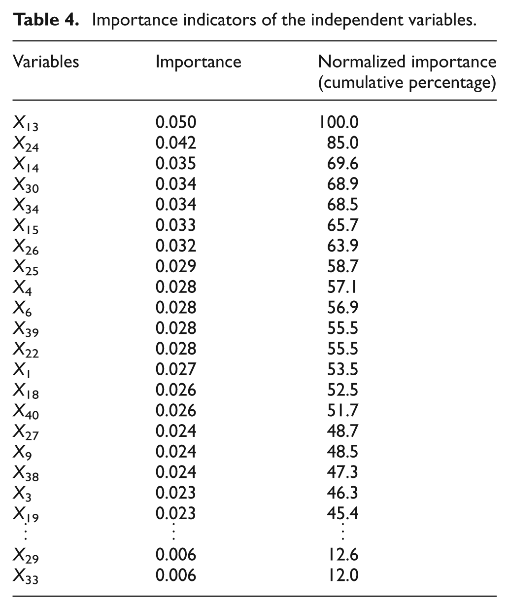
According to the importance indicators of the independent variables given in Table 4, the following conditions were adopted as the selection criteria to select 20 crucial attribute variables for the reduced model of the neural network: importance values should be greater than 0.2, and normalized importance values should be larger than 40%. Similarly, neural network analysis was performed on the 162 training group and 81 validation group data entries, achieving an accuracy rate of 100%, as shown in Table 5.

Table 5.

Prediction table of the neural network analysis.

	Normal (actual)	Abnormal (actual)	Accuracy rate
Training group
Normal	126	0	100%
Abnormal	0	36	100%
Validation group
Normal	61	0	100%
Abnormal	0	20	100%

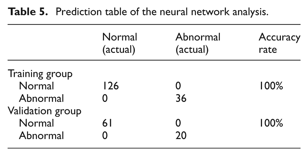
The full model of the neural network demonstrated a high accuracy rate in predicting the defect-free rate. Furthermore, the reduced model that adopted the first 20 questionnaire items with the highest contribution based on the importance indicators still demonstrated satisfactory predictability. This indicates that neural networks may also be effective in selecting the questionnaire items of audit quality scales for government procurement.

Comparison of results

The accuracy rate of the MTS, logistic regression, and neural network analyses is shown in Table 6. The reduced questionnaire model developed using the MTS to assess the Taipei City Government supply chain audit quality revealed an accuracy rate of 90.1% and 93.8% for the training and validation groups, respectively. Conversely, the reduced crucial attribute variable model developed using logistic regression showed an accuracy rate of 96.9% and 92.5% for the training and validation groups, respectively; the neural network analysis method showed an accuracy rate of 100% for both groups.

Table 6.

Comparison of accuracy among the analysis methods.

Analysis method	Training group	Validation group
MTS	90.1%	93.8%
Logistic regression	96.9%	92.5%
Neural networks	100%	100%

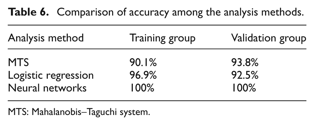
MTS: Mahalanobis–Taguchi system.

These three analysis methods were used to screen the key questionnaires. The MTS reduced the 50 original test items to 26, logistic regression reduced them to 18, and neural networks reduced them to 20. Table 7 shows that X₄, X₉, X₁₃, X₁₄, X₁₅, X₁₈, X₂₆, and X₃₈ were selected by all three analysis methods.

Table 7.

Key questionnaire for each analysis method.

Analysis method	Key questionnaire	Number of variables
MTS	X ₃, X₄, X₅, X₇, X₉, X₁₂, X₁₃, X₁₄, X₁₅, X₁₈, X₁₉, X₂₅, X₂₆, X₂₈, X₂₉, X₃₁, X₃₄, X₃₅, X₃₈, X₃₉, X₄₁, X₄₂, X₄₃, X₄₆, X₄₈, X₄₉	26
Logistic regression	X ₄, X₅, X₈, X₉, X₁₃, X₁₄, X₁₅, X₁₆, X₁₈, X₂₀, X₂₄, X₂₆, X₃₀, X₃₈, X₄₀, X₄₃, X₄₄, X₄₆	18
Neural networks	X ₁, X₃, X₄, X₆, X₉, X₁₃, X₁₄, X₁₅, X₁₈, X₁₉, X₂₂, X₂₄, X₂₅, X₂₆, X₂₇, X₃₀, X₃₄, X₃₈, X₃₉, X₄₀	20

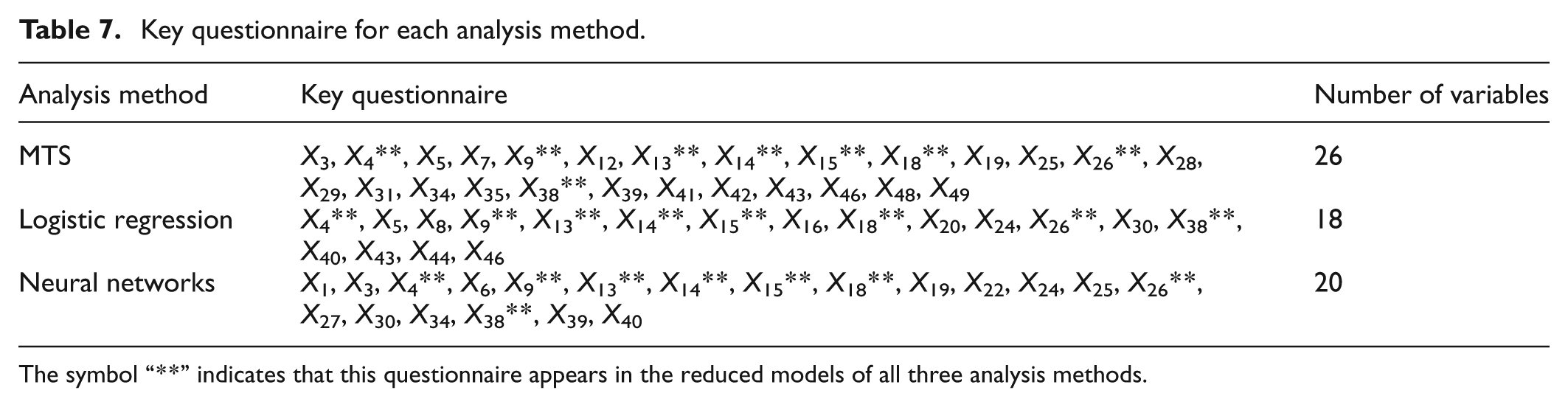
The symbol “**” indicates that this questionnaire appears in the reduced models of all three analysis methods.

These results indicate that when developing a reduced audit quality questionnaire model, the neural network method yields superior classification prediction accuracy than the traditional logistic regression analysis and the MTS. Nevertheless, the MTS method features high stability and an accuracy rate higher than 90%. Thus, the MTS, which involves using data mining and classification methods to reduce attribute variables for building prediction models, demonstrates high discrimination ability in practice.

Conclusion

The MTS, logistic regression, and neural network methods can all be used to classify imbalanced binary classification data. The prediction model developed by reducing attribute variables through feature selection showed that all three methods demonstrated favorable classification prediction accuracy. We reexamined the methods used for building audit quality questionnaire models to screen and reduce audit quality questionnaire items. The reduced models developed using the neural network analysis method featured high prediction accuracy rates, whereas those developed using the logistic regression analysis method possessed comparatively less attribute variables. Those developed using the MTS demonstrated high usability because such models not only showed the severity of the abnormal samples but also used the OAs and S/N ratio to test whether the variable selections were appropriate. The crucial attribute variables obtained from the screening process can be used to construct highly accurate and reduced classification prediction models, which are able to identify various classifications and are suitable for making classification predictions for various industries. Additionally, reducing the number of variables shortens prediction and identification times, rendering the models cost-effective.

Footnotes

Appendix 1

Table 8.

Variable numbers for the questionnaire items.

Number	Questionnaire item	Number	Questionnaire item
X ₁	Government procurement was divided into engineering procurement, financial procurement, and service procurement	X ₂₆	When review results exhibited variations, these results were submitted to committees and recorded
X ₂	Procurement thresholds were divided into thresholds of publication and supervision, as well as large and special procurement	X ₂₇	More than half of the committees attended the decision-making meeting; a notion was passed when approval was received from over half of the total number of committees
X ₃	Engineering procurement included air pollution prevention, material inspection or examination, and engineering management fees	X ₂₈	In cases where more than one tenderers were selected, price negotiation was performed according to the rank of tenderers
X ₄	Documents were made available for public viewing when fees for engineering procurement exceeded the threshold of supervision	X ₂₉	Period between the date when reserve price was approved and the date of tender opening was not too long
X ₅	Reasons for restricted tender were detailed and outlined (e.g. intellectual property rights)	X ₃₀	Planning units proposed estimated values and analyzed data
X ₆	Most advantageous tender selected were suitable for people who require this tender	X ₃₁	Tenderers who offered a price 80% lower than the reserve price explained and paid the price difference bond
X ₇	Selection items, evaluation criteria, and assessment methods were specified	X ₃₂	Procurement exceeding NT$ 100,000 are made public or posted in tender announcements
X ₈	Scores or ratings were given based on total scores, unit price, and rank	X ₃₃	Vendors paid the performance bond within 15 days starting from the second day of the final tender
X ₉	Name list of evaluation committees was kept confidential before review	X ₃₄	Contract was processed within 10 days starting from the second day of the final tender
X ₁₀	Valuation committee was established before tendering	X ₃₅	Vendors should insure with an insurance company for labor safety and accident insurance fees
X ₁₁	At least one member of the work group was qualified to be a procurement staff	X ₃₆	In cases where changes in contracts were a result of design or construction errors or negligence, the involved party should be responsible
X ₁₂	Content concerning qualification of tendering vendors was consistent in tender announcements and instructions or notices of tenders	X ₃₇	During the acceptance process, vendors submitted completed drawings and lists relevant to settlements
X ₁₃	Basic qualification of vendors was specified based on relevancy to tender targets and ability to execute aspects specified in an agreement	X ₃₈	Repair and maintenance were performed within a limited period of time when new defects were found during reinspection
X ₁₄	Review was conducted according to regulations each time a tender for engineering procurement failed or was canceled	X ₃₉	Chief inspector and assistant inspector were assigned (designer or supervisory personnel)
X ₁₅	Changes made to tendering documents during announcement period were reported to and approved by the head of the agency	X ₄₀	Responsible agency or authority recorded the acceptance process and result
X ₁₆	Date in the tender announcement was consistent with the performance period indicated in the contract	X ₄₁	A settlement and acceptance document was completed within 15 days once the acceptance of the project was approved
X ₁₇	Retendering was processed after failed or rejected tendering	X ₄₂	Vendors were responsible for any occurrence of defects or defaults during the warranty period to make improvements within a limited period of time
X ₁₈	Each page of the tender document was stamped	X ₄₃	At least one superintendent was assigned for projects amounting between NT$ 50 million and 200 million
X ₁₉	Outdated or invalid data were not incorporated into tender documents	X ₄₄	Responsible agency upon identifying defects or deficiencies notified vendors to make improvements within a limited period of time
X ₂₀	Supervision operations were arranged for tender opening procedures	X ₄₅	Inspection unit upon identifying defects or deficiencies notified vendors to make improvements within a limited period of time
X ₂₁	Enquiries regarding blacklisted vendors were made before opening of tender	X ₄₆	Inspection units executed quality auditing, supervised construction progress, and compiled construction inspection reports
X ₂₂	Tender documents included time, location, and names or codes of tendering vendors	X ₄₇	Contractors stipulated criteria for quality management
X ₂₃	Vendor qualification was reviewed in accordance with tender documents	X ₄₈	Contractor developed test procedures for materials and constructions
X ₂₄	Names, occupations, and professions of staffs in work groups were presented	X₄₉	Contractor implemented internal quality control
X ₂₅	Differences in selection items between vendors were presented	X ₅₀	In response to urgent incidents, restrictive tender was adopted

Declaration of conflicting interests

The authors declare that there is no conflict of interest.

Funding

This study was financially supported by the National Science Council of Taiwan under Grant NSC 102-2410-H-216-005 and Grant NSC 9-2632-H-216-001-MY2.

References

Hsiao

. An evaluation of the robustness of MTS for imbalanced data—a case study on the mobile phone test process. Master’s Thesis, National Chiao Tung University, Hsinchu, Taiwan, 2005.

Lai

. Data mining applied to the predictive model of triage system in emergency department: a case of medical center in Taiwan. Master’s Thesis, National Chin-Yi University of Technology, Taichung, Taiwan, 2007.

Perzyk

Biernacki

Kozlowski

. Data mining in manufacturing: significance analysis of process parameters. Proc IMechE, Part B: J Engineering Manufacture 2008; 222(11): 1503–1516.

Srinivas Harding

. A data mining integrated architecture for shop floor control. Proc IMechE, Part B: J Engineering Manufacture 2008; 222(5): 605–624.

Song

Kusiak

. Optimising product configurations with a data-mining approach. Int J Prod Res 2009; 47(7): 1733–1751.

. Constructing a compound classification model based on features selection: an empirical study on credit scoring. PhD Thesis, National Tsing Hua University, Hsinchu, Taiwan, 2010.

Wang

. Analysis of MTS: application of credit scoring. PhD Thesis, National Chiao Tung University, Hsinchu, Taiwan, 2003.

Lin

. Applying MTS to healthcare diagnosis—a case study on pressure ulcer. Master’s Thesis, National Tsing Hua University, Hsinchu, Taiwan, 2009.

Peng

. Applying MTS to improve tablet PC testing process. Master’s Thesis, Chung Hua University, Hsinchu, Taiwan, 2013.

10.

Taguchi

Jugulum

. New trends in multivariate diagnosis. Sankhya 2000; 62: 233–248.

11.

Riho

Suzuki

Oro

. The yield enhancement methodology for invisible defects using the MTS method. IEEE T Semiconduct M 2005; 18: 561–568.

12.

. Quality engineering. Taipei, Taiwan: Chinese Society for Quality, 2002.

13.

Berkson

. Application of the logistic function to bio-assay. J Am Stat Assoc 1944; 39(227): 357–365.

14.

Chang

. A study on prediction model of financial crisis by MTS—taking electronic companies in Taiwan as an example. Master’s Thesis, Chung Hua University, Hsinchu, Taiwan, 2007.

15.

Srinivisan

. A conjunctive-compensatory approach to the self-explication of multiattributed preference. Decision Sci 1987; 19: 295–305.

16.

Harrell

Lee

. A comparison of the discrimination of discriminant analysis and logistic regression under multivariate normality. In: PK

Sen

(ed.) Statistics in biomedical, public health and environmental sciences. Amsterdam: Elsevier, 1985, pp.333–343.

17.

Pan

Lee

. Finding and optimising the key factors for the multiple-response manufacturing process. Int J Prod Res 2009; 47(9): 2327–2344.

18.

Saygin

Mohan

Sarangapani

. Real-time detection of grip length during fastening of bolted joints: a Mahalanobis–Taguchi system (MTS) based approach. J Intell Manuf 2010; 21(4): 377–392.

19.

Tam

Kiang

. Managerial applications of neural network: the case of bank failure prediction. Manage Sci 1992; 23: 926–947.

20.

Zhang

. A chi-squared goodness-of-fit test for logistic regression models based on case-control data. Biometrika 1999; 86: 531–539.

21.

McCulloch

Pitts

. A logical calculus of the ideas immanent in nervous activity. B Math Biophys 1943; 5: 115–133.

22.

Rosenblatt

. The perceptron: a probabilistic model for information storage and organization in the brain, Cornell Aeronautical Laboratory. Psychol Rev 1958; 65(6): 386–408.

23.

Zhang

Patuwo

. Artificial neural networks in bankruptcy prediction: general framework and cross validation analysis. Eur J Oper Res 1999; 116: 16–32.

24.

Zhang

. Neural network. Taipei, China: Tung Hua Bookstore, 2005.

25.

Kuo

Hsu

Fang

. Automatic defect inspection system of colour filters using Taguchi-based neural network. Int J Prod Res 2013; 51(5): 1464–1476.

26.

Teng

Yang

Hsieh

. Optimization of wire electrical discharge machining of pure tungsten using neural network and response surface methodology. Proc IMechE, Part B: J Engineering Manufacture 2011; 225(6): 841–852.

27.

Hsieh

. The application of neuron network to the forecasting of a make to stock paper production system. Master’s Thesis, National Taiwan University of Science and Technology, Taipei, Taiwan, 2007.

28.

Kong

. Reducing test items of TFT-LCD product by using neural networks. Master’s Thesis, National Chiao Tung University, Hsinchu, Taiwan, 2007.

29.

Chang

Liu

. A new approach for manufacturing forecast problems with insufficient data: the case of TFT–LCDs. J Intell Manuf 2013; 24(2): 225–233.

30.

Lin

. The use of the Taguchi method with grey relational analysis and a neural network to optimize a novel GMA welding process. J Intell Manuf 2012; 23(5): 1671–1680.

Using Mahalanobis–Taguchi system,logistic regression,and neural network method to evaluate purchasing audit quality

Abstract

Keywords

Introduction

Literature review

MTS

MD

Orthogonal array

Signal-to-noise ratio

Logistic regression

Neural networks

Research and analysis

MTS analysis

Logistic regression analysis

Neural network analysis

Comparison of results

Conclusion

Footnotes

Appendix 1

Declaration of conflicting interests

Funding

References