A cost–benefit framework for assessing advanced manufacturing technology development: A case study

Abstract

Development of new advanced manufacturing technology for the aerospace industry is critical to enhance the manufacture and assembly of aerospace products. This article presents, verifies and validates a cost–benefit forecasting framework for the initial stages of advanced manufacturing technology development. The framework improves the decision-making process of which potential advanced manufacturing technologies to select and develop from concept to full-scale demonstration. Cost is the first element and is capable of forecasting the advanced manufacturing technology development effort in person-hours and cost of hardware using two parametric cost models. Benefit is the second element and forecasts the advanced manufacturing technology tangible and intangible performance. The proposed framework plots these quantified cost–benefit parameters to present development value advice for a diverse range of advanced manufacturing technologies. A detailed case study evaluating a total of 23 novel aerospace advanced manufacturing technologies verifies the capability and high accuracy of the framework within a large aerospace manufacturing organisation. Further validation is provided by quantifying the responses from 10 advanced manufacturing technology development experts, after utilising the methodology within an industrial setting. The case study demonstrates that quantifying the cost-benefit parameters provides the ability to select advanced manufacturing technologies that generate the best value to a business.

Introduction

Industrialised companies are constantly striving to improve their competitive capability and lower production costs by investing in new or proven advanced manufacturing technologies (AMTs). Managers are faced with the decision whether to invest in a new AMT, when benefits are hard to justify and the cost of development is vague and imprecise. ¹ This article presents a cost–benefit forecasting framework capable of improving the selection process of which AMTs to develop from concept to full-scale demonstration. The framework quantifies AMT development effort in person-hours and cost of hardware. These outputs are then plotted against the tangible and intangible forecast performances, graphically illustrating cost–benefit outputs. Quantifying the cost–benefit parameters provides aerospace manufacturing research and technology (R&T) with the ability to select the AMTs that generate the best value to a business. This is essential when research budgets are regularly cut and value for money is determined crucial. ² The forecasting framework has been developed from an extensive literature review and a detailed evaluation of the aerospace manufacturing industry, using interviews and workshops. The technology readiness level (TRL) maturity platform has been used to structure the framework. NASA developed the original TRL scale consisting of nine levels of classification, ranging from ‘basic principles observed and reported’ (TRL1) to ‘actual system through successful mission operations’ (TRL9). ³ This TRL scale has now been developed and adapted to suit the aerospace manufacturing industry, including manufacturing capability readiness levels (MCRLs) ⁴ and manufacturing readiness levels (MRLs).^5–7 However, both the MRL and MCRL development processes directly cross reference the original TRL, making the TRL a suitable platform for this research.^4,5,7,8 The development effort and cost are forecast within the framework to TRL6, the level an AMT must be proven to full scale within R&T. Beyond TRL6, the AMT is transitioned from R&T to manufacturing engineering operations.^9,10 Benefits are forecast within the framework to TRL7-9, the point of R&T handover to manufacturing operations. The cost forecasting element of the framework has been verified using 15 novel AMTs within manufacturing R&T. The benefit forecasting aspect has been verified using eight AMTs with known conclusions. Further validation has been provided by detailed responses from 10 AMT development experts.

The remaining sections of this article are structured in the following format: section ‘Related research’ summarises research related to development cost estimation and benefit forecasting of AMTs. Section ‘Proposed framework’ details the developed cost–benefit framework stages, including the mathematical notation. Section ‘Framework case study’ presents a case study including the evaluation of 15 AMTs. Section ‘Framework verification’ details the high accuracy of the framework using statistical verification. Section ‘Framework validation’ presents the responses of 10 AMT experts. Section ‘Conclusion’ discusses the framework strengths, weaknesses and recommendations for future work.

Related research

The majority of existing literature can be placed into two categories: AMT development cost estimation and AMT benefit forecasting. When referencing AMT development cost estimation, there is a lack of existing literature for forecasting AMT development effort in person-hours and cost of hardware. To respond, focus was placed on general cost models and techniques, with a refinement to the TRL. This helped to define existing research from a similar domain and provide a platform to systematically cross reference, helping solve the AMT development cost estimation problem.

In cost estimation of TRLs within systems engineering, research so far has typically focused on costing the product for delivery into a system. ¹¹ Further systems engineering research has been conducted by Valerdi ¹² who created a systems engineering cost model. This model is capable of forecasting systems engineering effort in person-months and utilised the TRL as a multiplicative factor. Significant emphasis has been placed on using the TRL as a metric for cost estimation, although no existing research has addressed the cost drivers for technology development.^13,14 One study utilised the TRL metric to adjust existing commercially available cost estimation models for space programs, although only evaluated using historical development time. ¹⁵ Existing commercial tools only estimate development cost as a single element of overall hardware product cost. The TRL is used as part of an assumption to spread this estimated cost over the technology development cycle. Many commercial hardware cost estimation and resource forecasting models are now looking to integrate TRLs as a metric. However, these have not been implemented and are not taken into consideration when specifically analysing the development of AMTs.^15–17

Benefit forecasting or performance evaluation of aerospace AMTs is the second relevant research domain. Despite a superior level of available literature, this domain has a high level of focus placed on evaluation from purely an economic perspective.^18–20 Ordoobadi ¹⁹ addresses this issue to distinguish between AMT alternatives with similar financial results using Taguchi’s loss function. This is achieved by the decision maker estimating the benefit priority and aligning with the required goals of the AMT. These are collated using Taguchi loss functions, quantitatively evaluating alternative AMTs. A further AMT justification toolset was developed using system-wide benefits value analysis (SWBVA) and also moved away from the traditional economic financial analysis. ²⁰ This toolset is utilised if the AMT is not economically justified. Users follow a structured procedure to evaluate the system-wide benefits, defining if they are sufficient to justify the calculated gap. Almannai et al. ²¹ developed a decision-making toolset for application to manufacturing automated technology selection. This toolset utilised quality function deployment (QFD) in affiliation with failure mode and effect analysis (FMEA). Its aim was to select the most effective manufacturing automation solution and correlate the risks. Evans et al. ²² developed a justification method for evaluation of manufacturing technologies for use within manufacturing systems. This technique applied fuzzy decision trees to establish patterns using a case repository. Elaboration of this research captured expert knowledge and experience of a decision maker when making future selection decisions. ²³

In summary, existing research and detailed discussions with experts inside the aerospace manufacturing sector identified the lack of available research for forecasting AMT development effort and cost, at the initial development stages. Despite availability of performance evaluation for AMTs, there is no specific toolset to quantify both tangible and intangible AMT performances at the early development stages. When combining cost and benefit forecasting of AMTs, there is currently no suitable toolset or framework capable of quantifying these parameters at the initial stages of development. Therefore, there is a need to develop a novel framework in this area. This framework should be capable of forecasting AMT development effort and cost to TRL6. Furthermore, the framework must be capable of forecasting the tangible and intangible benefits to the point of AMT implementation into manufacturing operations, TRL7-9. The final cost–benefit outputs of the forecasting framework must be graphically represented to identify which AMTs provide the business with the best value, enhancing the R&T investment decision.

Proposed framework

This section presents the proposed cost–benefit framework for forecasting novel aerospace AMT development effort and benefit, at the conceptual stages of maturity. An overview of the framework is presented in Figure 1, with each stage detailed in the proceeding sub sections. The framework is then used for evaluation of 15 novel AMTs, with the results presented in section ‘Framework case study’.

Figure 1.

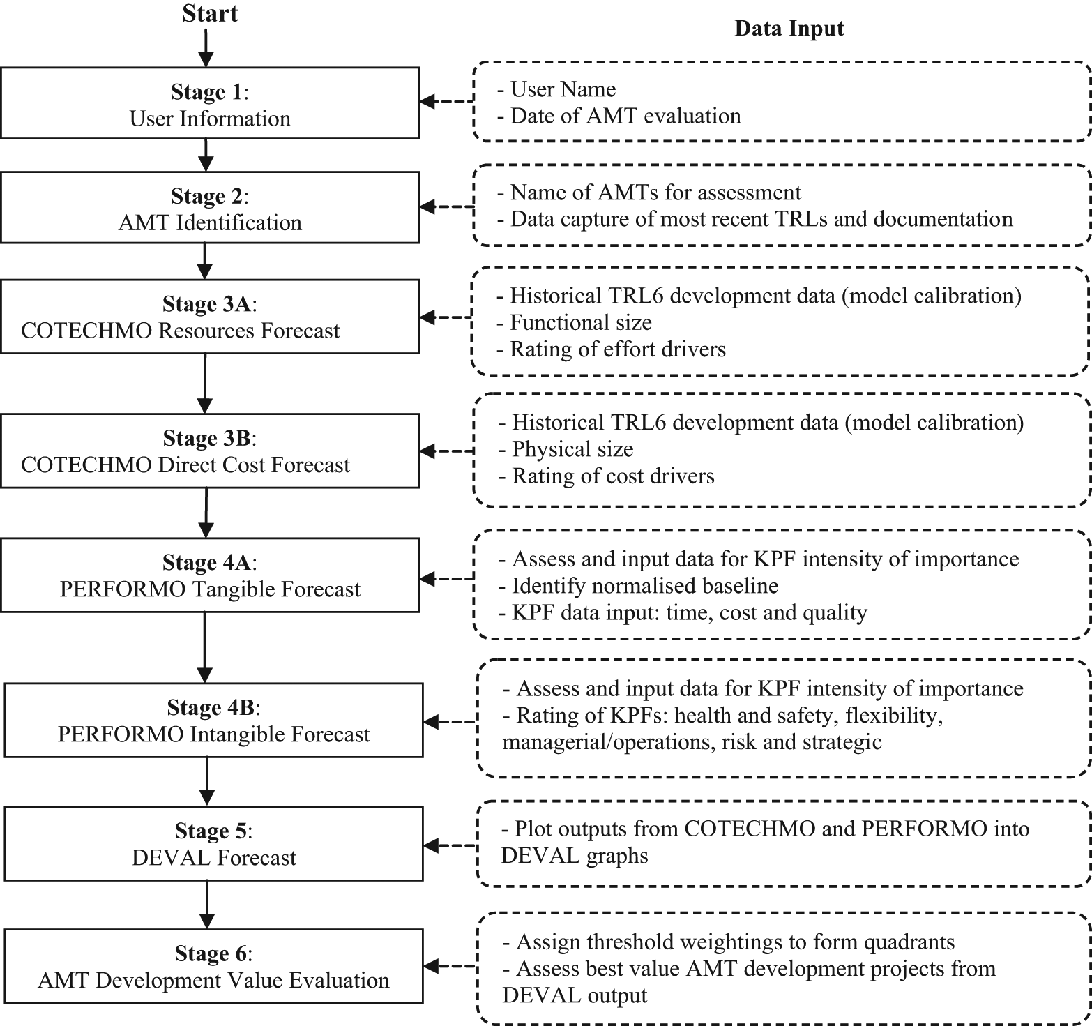
Proposed aerospace AMT development cost–benefit forecasting framework.

Stage 1 − user information

Stage 1 of the framework involves the user inputting their name and date of the AMT evaluation. This records their details and location within the business, providing full traceability of decisions made at the initial development stages.

Stage 2 − AMT identification

Stage 2 involves selecting AMTs within the business for assessment from a manufacturing R&T portfolio. This is typically performed with a manager who oversees the portfolio of AMTs suitable for assessment.

Stage 3A − COTECHMO resources (person-hours) forecast

Stage 3A involves the operation of the developed parametric ‘Constructive Technology Development Cost Model’ (COTECHMO) resources toolset and forecasts AMT development resources (person-hours) to TRL6. The mathematical notation of the model is presented in the proceeding part of this subsection. When evaluating the overall COTECHMO resources model cost estimating relationship (CER), distinction must be made between size and effort drivers. The size driver is additive and the effort driver is multiplicative, each represented in equation (1)

$$\mathrm{PH}=A\times \left(\mathrm{Size}\right)\times \left(\mathrm{EM}\right)$$

(1)

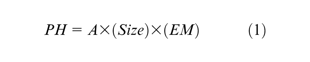
where PH is person-hours (effort in resources); A is calibration factor; Size is size drivers counting the AMT process functional size (additive) and EM is effort multipliers impacting AMT development effort (multiplicative).

Equation (2) is the final COTECHMO resources parametric CER and is broken down into 3 size drivers (predictors) and 13 effort drivers (effort multipliers)

$$\mathrm{PH}=A·(\sum _k{\omega }_e{\varphi }_e+{\omega }_n{\varphi }_n+{\omega }_d{\varphi }_d)·{\displaystyle \underset{j=1}{\overset{13}{\Pi }}}{\mathrm{EM}}_j$$

(2)

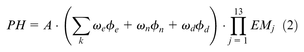
where PH is person-hours (effort in resources); A is historical data calibration factor; $k$ is number of geometric requirements, number of process steps and number of test pieces; $\omega$ is weighting, $e$ is easy, $n$ is nominal, $d$ is difficult; $\varphi$ is size driver count and ${\mathrm{EM}}_j$ represents the effort multipliers, with each set to a nominal value of 1.0.

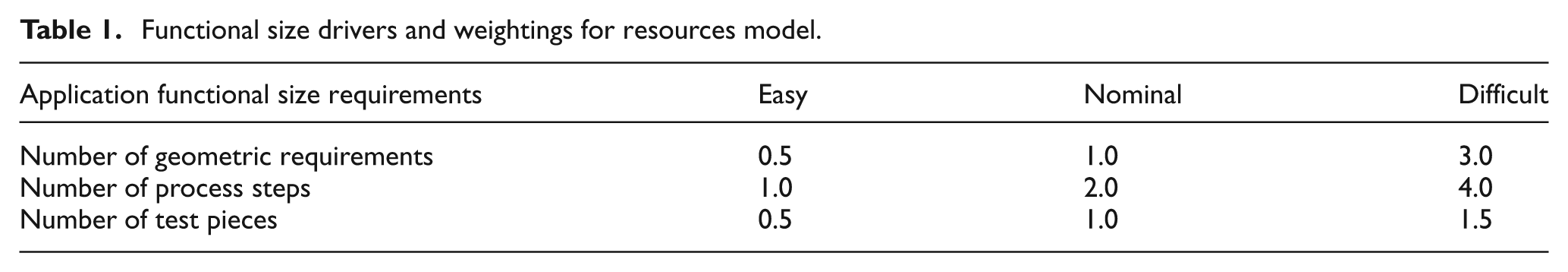
The size drivers are listed in Table 1 with their relative rating and weightings. The impact of an individual effort multiplier is the range of the highest to the lowest, indicated by the effort multiplier ratio (EMR) listed in Table 2.

Table 1.

Functional size drivers and weightings for resources model.

Application functional size requirements	Easy	Nominal	Difficult
Number of geometric requirements	0.5	1.0	3.0
Number of process steps	1.0	2.0	4.0
Number of test pieces	0.5	1.0	1.5

Table 2.

Effort driver ratings and effort multipliers for resources model.

Effort driver name	Very low	Low	Nominal	High	Very high	EMR
Product application experience	1.85	1.36	1.00	0.77	0.60	3.08
Degree of process novelty	0.62	0.79	1.00	1.36	1.85	2.98
Process experience	1.64	1.28	1.00	0.81	0.65	2.52
Test piece material complexity	0.65	0.81	1.00	1.22	1.50	2.31
Requirements understanding	1.50	1.22	1.00	0.81	0.65	2.31
Manufacturing documentation of requirements	1.50	1.22	1.00	0.81	0.65	2.31
TRL pack experience	1.48	1.22	1.00	0.82	0.67	2.21
Supplier network availability and capability	1.39	1.18	1.00	0.85	0.72	1.93
Installation complexity	0.76	0.87	1.00	1.21	1.47	1.93
Location variation of trials and tests	0.76	0.87	1.00	1.21	1.47	1.93
Production rate reduction requirements	0.60	0.77	1.00	1.37	1.87	1.67
Required development schedule	1.66	1.20	1.00	1.13	1.28	1.29
Datum complexity	–	–	1.00	1.13	1.28	1.28

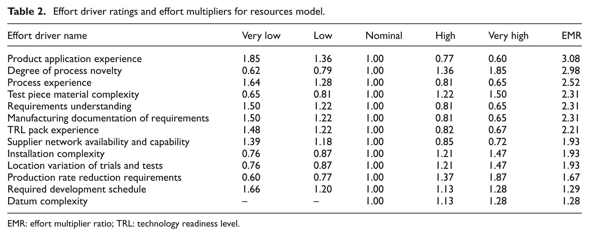
EMR: effort multiplier ratio; TRL: technology readiness level.

The size drivers form the additive part of the CER and quantify the functional size of the AMT process for its assigned application. This technique has used function point (FP) analysis, which is widely used within software engineering^24,25 and adapted using a similar technique to Valerdi ¹² for application to systems engineering. Size drivers are counted and adjusted based on the complexity of the requirement, ranging from easy to difficult. The size drivers are listed with their relative complexity weightings in Table 1. Table 2 lists the effort drivers and their ratings, which range from ‘very low’ to ‘very high’. The ratings for each of the effort multipliers have been listed based on their EMR. EMR identifies the variability of the driver and its individual influence on development person-hours. The quantified size and effort driver weightings were finalised from a ‘two-stage Wideband Delphi study’ using 21 AMT development experts and 4 cost estimation experts.

Stage 3B − COTECHMO direct cost forecast

Stage 3B involves the operation of the developed parametric COTECHMO direct cost toolset and forecasts AMT development direct (hardware) cost to TRL6. The mathematical notation of the model is presented in the following part of this subsection. The COTECHMO direct cost model equation form uses additive (physical hardware size) and multiplicative (development complexity), presented in equation (3)

$$\mathrm{DC}=A\times \left(\mathrm{Size}\right)\times \left(\mathrm{CM}\right)$$

(3)

where DC is development direct cost (€); A is calibration factor; Size is the measure of physical hardware size of the AMT process in volume (additive); CM is cost multipliers that impact AMT development direct cost (multiplicative).

Equation (4) is the final COTECHMO direct cost parametric CER and is broken down into 1 size driver (predictor) and 13 cost drivers (cost multipliers)

$$\mathrm{DC}=A·(x,y,z)·{\displaystyle \underset{j=1}{\overset{13}{\Pi }}}{\mathrm{CD}}_j$$

(4)

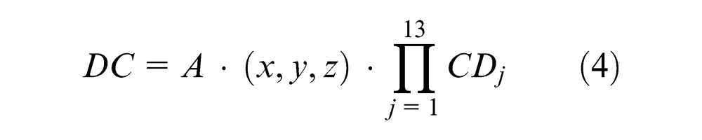
where DC is development cost (€); A is historical data calibration factor; $x$ is width of the AMT process hardware; $y$ is length of the AMT process hardware; $z$ is height of AMT process hardware and ${\mathrm{CD}}_j$ represent the cost multipliers, with each set to a nominal value of 1.0. The impact of an individual cost multiplier is the range of the highest to the lowest, indicated by the cost multiplier ratio (CMR) listed in Table 3.

Table 3.

Cost driver ratings and cost multipliers for the direct cost model.

Cost driver name	Very low	Low	Nominal	High	Very high	CMR
Number of geometric accuracy requirements	0.40	0.60	1.00	1.60	1.87	4.67
Degree of process novelty	0.50	0.70	1.00	1.49	1.90	3.80
Automation level requirements	0.60	0.81	1.00	1.60	1.90	3.17
Tooling requirements	0.55	0.70	1.00	1.30	1.60	2.91
Number of process steps	0.67	0.82	1.00	1.48	1.85	2.76
Process capability requirements	0.67	0.82	1.00	1.48	1.85	2.76
Test piece material complexity	0.60	0.72	1.00	1.18	1.39	2.32
Metrology requirements	0.60	0.72	1.00	1.18	1.39	2.32
Production rate reduction requirements	–	–	1.00	1.40	1.92	1.92
Human factors requirements	0.72	0.85	1.00	1.10	1.20	1.67
Manufacturing environment requirements	0.81	0.90	1.00	1.10	1.27	1.57
Installation complexity	0.81	0.90	1.00	1.10	1.27	1.57
Process test and verification requirements	0.81	0.90	1.00	1.10	1.27	1.57

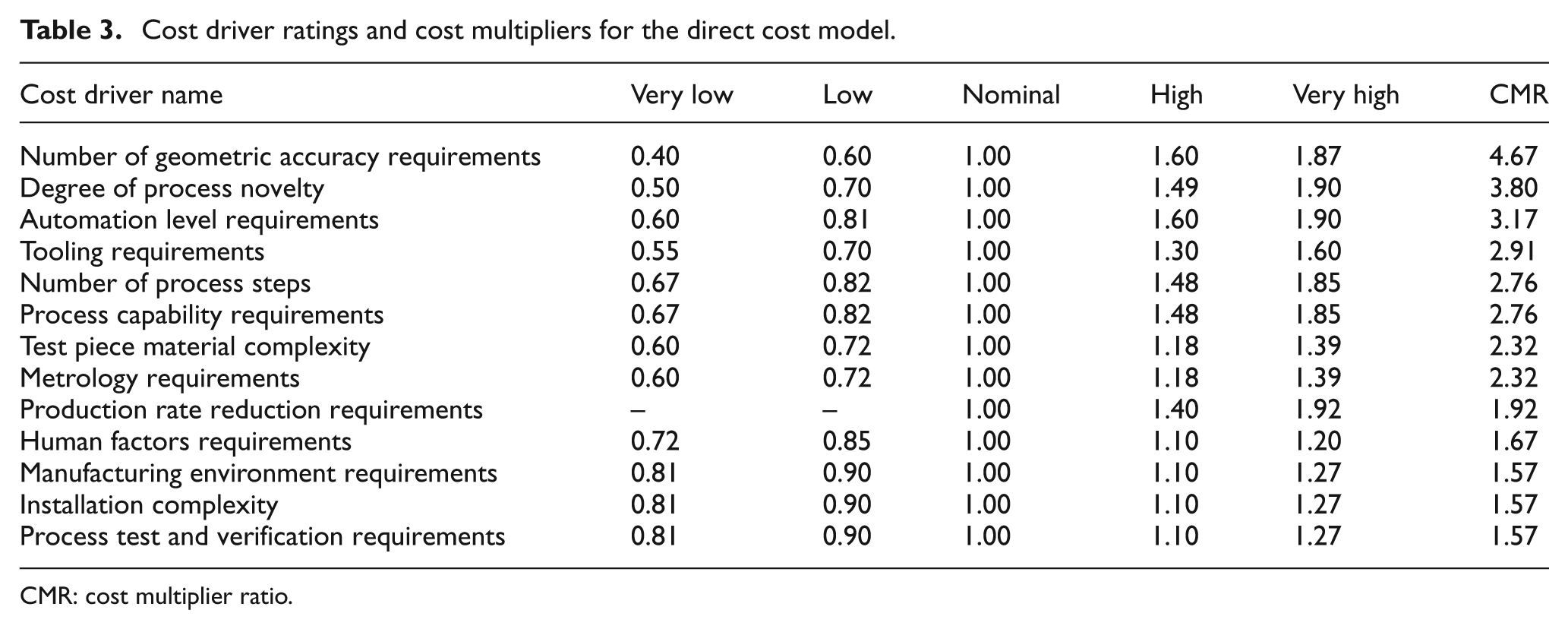
CMR: cost multiplier ratio.

The model consists of one size driver that forms the additive part of the CER to quantify the physical volume of the AMT process hardware for its assigned application. Table 3 lists the model cost multipliers with their relative ratings, which range from ‘very low’ to ‘very high’. The ratings for each of the cost drivers have been listed based on their CMR. CMR identifies the variability of the driver and its individual influence on development direct cost. The quantified cost multiplier weightings were finalised from a ‘two-stage Wideband Delphi study’ conducted using 21 AMT development experts and 4 cost estimation experts.

Stage 4A − PERFORMO tangible forecast

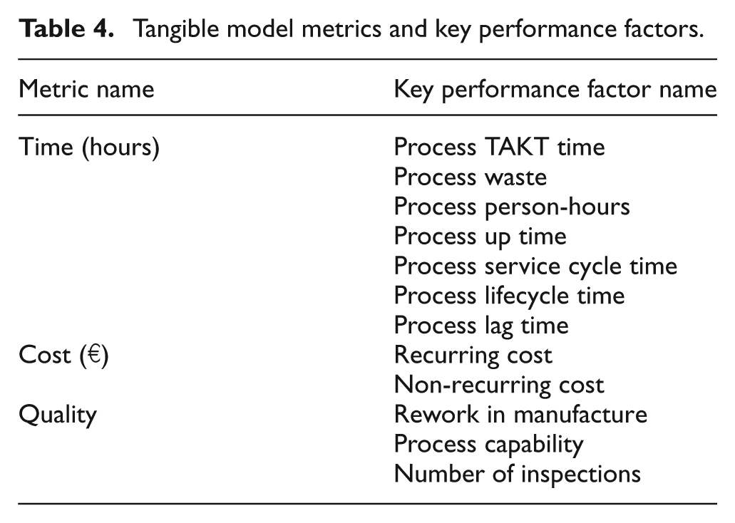
Stage 4A involves the operation of the developed ‘Performance Forecasting Model’ (PERFORMO) tangible toolset. The model forecasts AMT tangible performance to the point of full implementation into manufacturing operations at TRL7-9. The model algorithm consists of three performance metrics: time, cost and quality. Each metric is broken down into key performance factors (KPFs), with the time metric broken down into seven KPFs, the cost metric two KPFs and the quality metric three KPFs, listed in Table 4.

Table 4.

Tangible model metrics and key performance factors.

Metric name	Key performance factor name
Time (hours)	Process TAKT time
	Process waste
	Process person-hours
	Process up time
	Process service cycle time
	Process lifecycle time
	Process lag time
Cost (€)	Recurring cost
	Non-recurring cost
Quality	Rework in manufacture
	Process capability
	Number of inspections

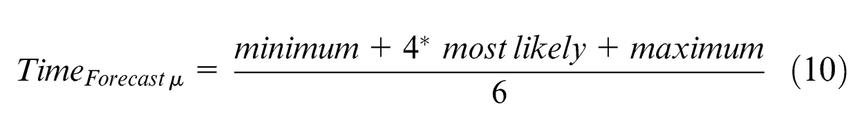
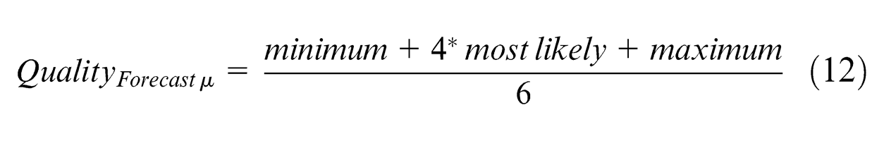
Equations (5)–(7) identify how the time, cost and quality baselines are divided by the mean forecast performance for 10 of the 12 KPFs. In contrary, ‘Process Lifecycle Time’ and ‘Process Capability’ KPFs have their mean forecast performance divided by the baseline, shown in equations (8) and (9). A performance enhancement for these two KPFs has a larger value, not a reduction followed with the other ten KPFs. The mean forecast performance for each KPF is calculated using a three-point estimate with a beta distribution, presented in equations (10)–(12)

$${\mathrm{Time}}_j=\frac{{\mathrm{Time}}_{\mathrm{Baseline}}}{{\mathrm{Time}}_{\mathrm{Forecast}\mu }}$$

(5)

$${\mathrm{Cost}}_j=\frac{{\mathrm{Cost}}_{\mathrm{Baseline}}}{{\mathrm{Cost}}_{\mathrm{Forecast}\mu }}$$

(6)

$${\mathrm{Quality}}_j=\frac{{\mathrm{Quality}}_{\mathrm{Baseline}}}{{\mathrm{Quality}}_{\mathrm{Forecast}\mu }}$$

(7)

$${\mathrm{Time}}_j=\frac{{\mathrm{Time}}_{\mathrm{Forecast}\mu }}{{\mathrm{Time}}_{\mathrm{Baseline}}}$$

(8)

$${\mathrm{Quality}}_j=\frac{{\mathrm{Quality}}_{\mathrm{Forecast}\mu }}{{\mathrm{Quality}}_{\mathrm{Baseline}}}$$

(9)

where

$${\mathrm{Time}}_{\mathrm{Forecast}\mu }=\frac{\mathrm{minimum}+4^{*}\mathrm{most}\mathrm{likely}+\mathrm{maximum}}{6}$$

(10)

$${\mathrm{Cost}}_{\mathrm{Forecast}\mu }=\frac{\mathrm{minimum}+4^{*}\mathrm{most}\mathrm{likely}+\mathrm{maximum}}{6}$$

(11)

$${\mathrm{Quality}}_{\mathrm{Forecast}\mu }=\frac{\mathrm{minimum}+4^{*}\mathrm{most}\mathrm{likely}+\mathrm{maximum}}{6}$$

(12)

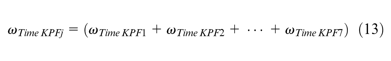
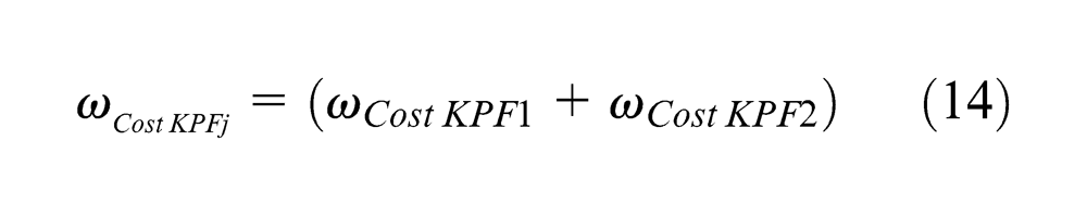
Within the model, final outputs from equation (5)–(9) are multiplied by the weighting of each KPF selected by the model user. This defines the importance of each KPF for the AMT selected for evaluation. The total weighting for each time KPF is presented in equation (13), the KPFs weighting for cost in equation (14) and the quality KPFs in equation (15). Equation (16) categorises how the total weightings are normalised at 1 for all the KPFs combined, allowing comparison of a diverse range of AMTs.

$${\omega }_{\mathrm{Time}\mathrm{KPFj}}=({\omega }_{\mathrm{Time}\mathrm{KPF}1}+{\omega }_{\mathrm{Time}\mathrm{KPF}2}+\cdots +{\omega }_{\mathrm{Time}\mathrm{KPF}7})$$

(13)

$${\omega }_{\mathrm{Cost}\mathrm{KPFj}}=({\omega }_{\mathrm{Cost}\mathrm{KPF}1}+{\omega }_{\mathrm{Cost}\mathrm{KPF}2})$$

(14)

$${\omega }_{\mathrm{Quality}\mathrm{KPFj}}=({\omega }_{\mathrm{Quality}\mathrm{KPF}1}+{\omega }_{\mathrm{Quality}\mathrm{KPF}2}+{\omega }_{\mathrm{Quality}\mathrm{KPF}3})$$

(15)

$${\displaystyle \sum _{j=1}^7}{\omega }_{\mathrm{Time}\mathrm{KPFj}}+{\displaystyle \sum _{j=1}^2}{\omega }_{\mathrm{Cost}\mathrm{KPFj}}+{\displaystyle \sum _{j=1}^3}{\omega }_{\mathrm{Quality}\mathrm{KPFj}}=1$$

(16)

where $\omega$ is the weighting.

Therefore, the final equation form used within the PERFORMO tangible model is presented within equation (17)

$$\mathrm{TP}={\displaystyle \sum _{j=1}^7}{\omega }_{\mathrm{Time}\mathrm{KPFj}}·{\mathrm{Time}}_j+{\displaystyle \sum _{j=1}^2}{\omega }_{\mathrm{Cost}\mathrm{KPFj}}·{\mathrm{Cost}}_j+{\displaystyle \sum _{j=1}^3}{\omega }_{\mathrm{Quality}\mathrm{KPFj}}·{\mathrm{Quality}}_j$$

(17)

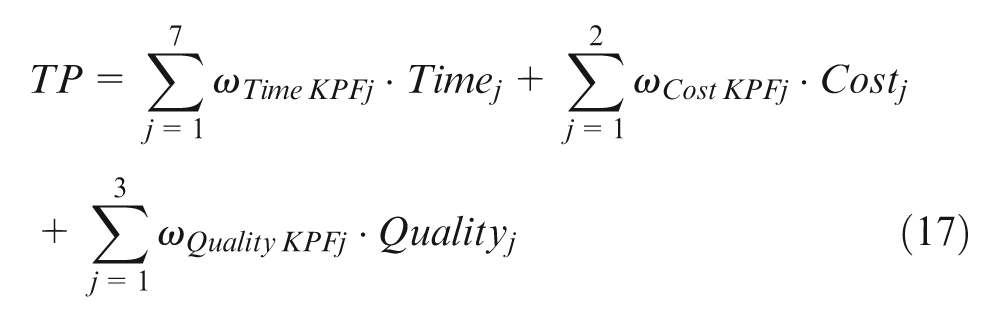
where TP is tangible performance; ${\omega }_{\mathrm{Time}\mathrm{KPFj}}$ is time KPF weightings; ${\omega }_{\mathrm{Cost}\mathrm{KPFj}}$ is cost KPF weightings; ${\omega }_{\mathrm{Quality}\mathrm{KPFj}}$ is quality KPF weightings; ${\mathrm{Time}}_j$ represents the time KPFs listed in Table 4 with each forecast from a baseline using either Equation (5) or (8); ${\mathrm{Cost}}_j$ represents the cost KPFs listed in Table 4 with each forecast from a baseline using Equation (6) and ${\mathrm{Quality}}_j$ represents the quality KPFs listed in Table 4 with each forecast from a baseline using Equation (7) or (9).

Stage 4B − PERFORMO intangible forecast

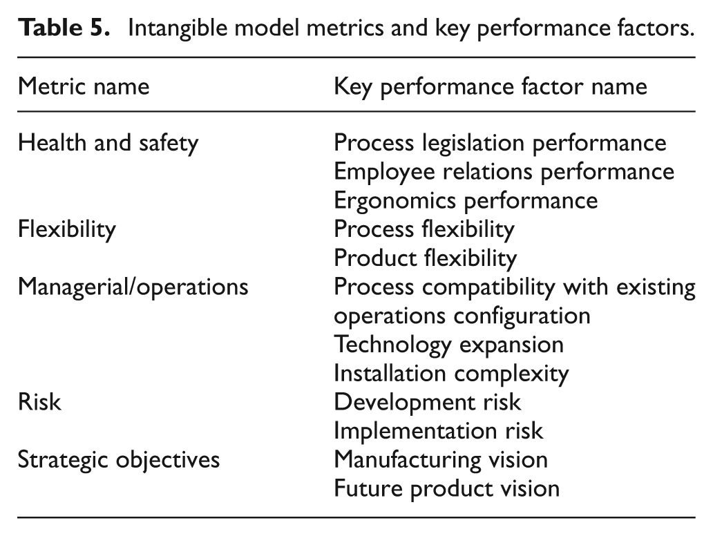
Stage 4B involves the operation of the developed PERFORMO intangible toolset for forecasting intangible performance to TRL7-9. The PERFORMO intangible model equation form consists of five performance metrics: health and safety, flexibility, managerial/operations, risk and strategic objectives. Each metric is broken down into KPFs. The health and safety metric is broken down into three KPFs, flexibility two KPFs, managerial three KPFs, risk and strategic objectives each having two KPFs, all listed in Table 5.

Table 5.

Intangible model metrics and key performance factors.

Metric name	Key performance factor name
Health and safety	Process legislation performance
	Employee relations performance
	Ergonomics performance
Flexibility	Process flexibility
	Product flexibility
Managerial/operations	Process compatibility with existing operations configuration
	Technology expansion
	Installation complexity
Risk	Development risk
	Implementation risk
Strategic objectives	Manufacturing vision
	Future product vision

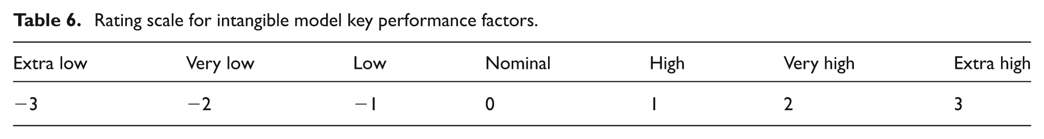
The rating scale for each KPF listed in Table 5 has a scale ranging from −3 to 3, presented in Table 6. These were quantified using 9 AMT development experts and 2 decision-making experts. This scale is multiplied by the weighting of each KPF defined by the model user, presented in equations (18)–(22). This defines the importance of each KPF for the AMT assessed

$${\omega }_{\mathrm{Health}\&\mathrm{Safety}\mathrm{KPFj}}=({\omega }_{H\&S\mathrm{KPF}1}+{\omega }_{H\&S\mathrm{KPF}2}+{\omega }_{H\&S\mathrm{KPF}3})$$

(18)

$${\omega }_{\mathrm{Flexibility}\mathrm{KPFj}}=({\omega }_{\mathrm{Flexibility}\mathrm{KPF}1}+{\omega }_{\mathrm{Flexibility}\mathrm{KPF}2})$$

(19)

$${\omega }_{\mathrm{Managerial}\mathrm{KPFj}}=({\omega }_{\mathrm{Managerial}\mathrm{KPF}1}+{\omega }_{\mathrm{Managerial}\mathrm{KPF}2}+{\omega }_{\mathrm{Managerial}\mathrm{KPF}3})$$

(20)

$${\omega }_{\mathrm{Risk}\mathrm{KPFj}}=({\omega }_{\mathrm{Risk}\mathrm{KPF}1}+{\omega }_{\mathrm{Risk}\mathrm{KPF}2})$$

(21)

$${\omega }_{\mathrm{Strategic}\mathrm{KPFj}}=({\omega }_{\mathrm{Strategic}\mathrm{KPF}1}+{\omega }_{\mathrm{Strategic}\mathrm{KPF}2})$$

(22)

where $\omega$ is the weighting.

Table 6.

Rating scale for intangible model key performance factors.

Extra low	Very low	Low	Nominal	High	Very high	Extra high
−3	−2	−1	0	1	2	3

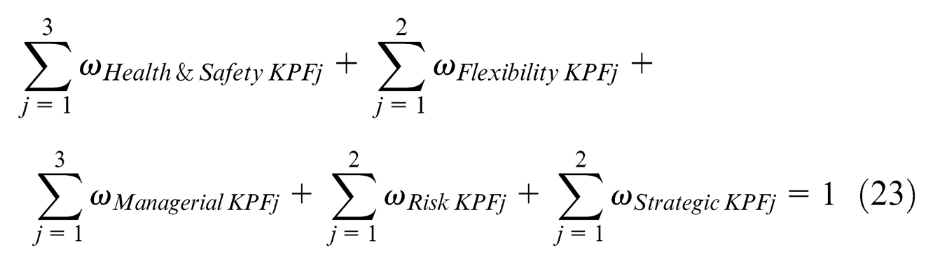
Equation (23) categorises how the total weightings are normalised at 1 for all KPFs combined. This allows for comparison of a variety of AMTs

$${\displaystyle \sum _{j=1}^3}{\omega }_{\mathrm{Health}\&\mathrm{Safety}\mathrm{KPFj}}+{\displaystyle \sum _{j=1}^2}{\omega }_{\mathrm{Flexibility}\mathrm{KPFj}}+{\displaystyle \sum _{j=1}^3}{\omega }_{\mathrm{Managerial}\mathrm{KPFj}}+{\displaystyle \sum _{j=1}^2}{\omega }_{\mathrm{Risk}\mathrm{KPFj}}+{\displaystyle \sum _{j=1}^2}{\omega }_{\mathrm{Strategic}\mathrm{KPFj}}=1$$

(23)

Therefore, the final PERFORMO intangible model is presented in equation (24)

$$\begin{array}{c}\multicolumn{1}{c}{\mathrm{IP}={\displaystyle \sum _{j=1}^3}{\omega }_{\mathrm{Health}\&\mathrm{Safety}\mathrm{KPFj}}·\mathrm{Health}\mathrm{and}{\mathrm{Safety}}_j}\\ \multicolumn{1}{c}{+{\displaystyle \sum _{j=1}^2}{\omega }_{\mathrm{Flexibility}\mathrm{KPFj}}·{\mathrm{Flexibility}}_j+{\displaystyle \sum _{j=1}^3}{\omega }_{\mathrm{Managerial}\mathrm{KPFj}}}\\ \multicolumn{1}{c}{·{\mathrm{Managerial}}_j+{\displaystyle \sum _{j=1}^2}{\omega }_{\mathrm{Risk}\mathrm{KPFj}}·{\mathrm{Risk}}_j}\\ \multicolumn{1}{c}{+{\displaystyle \sum _{j=1}^2}{\omega }_{\mathrm{Strategic}\mathrm{KPFj}}·{\mathrm{Strategic}}_j}\end{array}$$

(24)

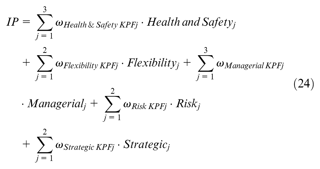
where IP is intangible performance; ${\omega }_{\mathrm{Health}\mathrm{and}\mathrm{Safety}\mathrm{KPFj}}$ is health and safety KPF weightings; ${\omega }_{\mathrm{Flexibility}\mathrm{KPFj}}$ is flexibility KPF weightings; ${\omega }_{\mathrm{Managerial}\mathrm{KPFj}}$ is managerial KPF weightings; ${\omega }_{\mathrm{Risk}\mathrm{KPFj}}$ is risk KPF weightings; ${\omega }_{\mathrm{Stategic}\mathrm{KPFj}}$ is strategic objective KPF weightings and $\mathrm{Health}\mathrm{and}{\mathrm{Safety}}_j,{\mathrm{Flexibility}}_j,{\mathrm{Managerial}}_j,{\mathrm{Risk}}_j,{\mathrm{Strategic}}_j$ represent the health and safety, flexibility, managerial, risk and strategic objective KPFs, listed in Table 5, with their rating scale and its corresponding value listed in Table 6.

Stage 5 − DEVAL forecast

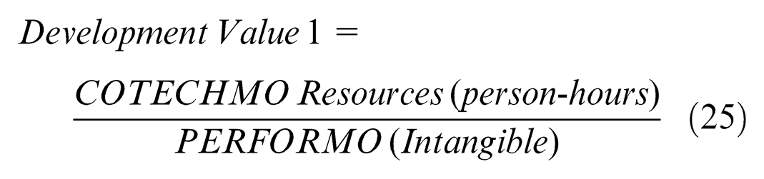
Stage 5 involves compiling data outputs from each COTECHMO and PERFORMO toolset and plotting into development value (DEVAL) advice graphs. This output provides the AMT portfolio assessor with data to illustrate the DEVAL of each selected AMT. AMT evaluation is presented by quantifying the ‘x-axis’, utilising each COTECHMO toolset (Stages 3A and 3B) and the ‘y-axis’ with each PERFORMO toolset (Stages 4A and 4B). The data are plotted within each DEVAL graph using the equation forms presented in equations (25)–(28)

$$\mathrm{Development}\mathrm{Value}1=\frac{\mathrm{COTECHMO}\mathrm{Resources}(\mathrm{person}-\mathrm{hours})}{\mathrm{PERFORMO}(\mathrm{Intangible})}$$

(25)

$$\mathrm{Development}\mathrm{Value}2=\frac{\mathrm{COTECHMO}\mathrm{Resources}(\mathrm{person}-\mathrm{hours})}{\mathrm{PERFORMO}\left(\mathrm{Tangible}\right)}$$

(26)

$$\mathrm{Development}\mathrm{Value}3=\frac{\mathrm{COTECHMO}\mathrm{Direct}\mathrm{Cost}(€)}{\mathrm{PERFORMO}\left(\mathrm{Tangible}\right)}$$

(27)

$$\mathrm{Development}\mathrm{Value}4=\frac{\mathrm{COTECHMO}\mathrm{Direct}\mathrm{Cost}(€)}{\mathrm{PERFORMO}(\mathrm{Intangible})}$$

(28)

Stage 6 − AMT DEVAL evaluation

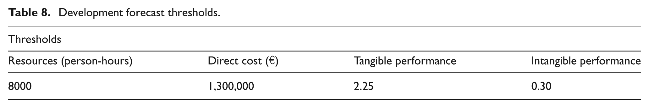
Within the final stage of the framework, the output from DEVAL is evaluated and assigned development effort and performance thresholds. Threshold values are defined with the experts or a manager overseeing the portfolio of AMTs and form quadrants. Quadrants identify which AMTs within the portfolio provide the best value with the available resources and cost budget limits. These are presented graphically within the section ‘Framework case study.’

Framework case study

To verify and validate outputs from each model and the cost–benefit framework, an industrial case study was followed using the 15 AMTs listed in Table 7. Each AMT was picked based on its technological and application diversity, vigorously testing each forecasting procedure. The 15 selected AMTs were run through the cost–benefit framework discussed in the previous section, with the following results.

Table 7.

Selected AMTs and development experts used for the cost–benefit framework case study.

AMT number	Expert number	Role	Years of AMT development experience
1	1	Machining research specialist	11
2	2	Metrology/manufacturing research engineer	6
3	3	Manufacturing research engineer	15
4	4	Automation specialist	4
5	5	Automation research engineer	20
6	1	Machining research specialist	11
7	6	Project leader	10
8	7	Manufacturing research engineer	15
9	8	Research portfolio manager	15
10	9	Manufacturing project manager	5
11	10	Manufacturing and materials research engineer	25
12	9	Manufacturing project manager	5
13	9	Manufacturing project manager	5
14	10	Manufacturing and materials research engineer	25
15	3	Manufacturing research engineer	15

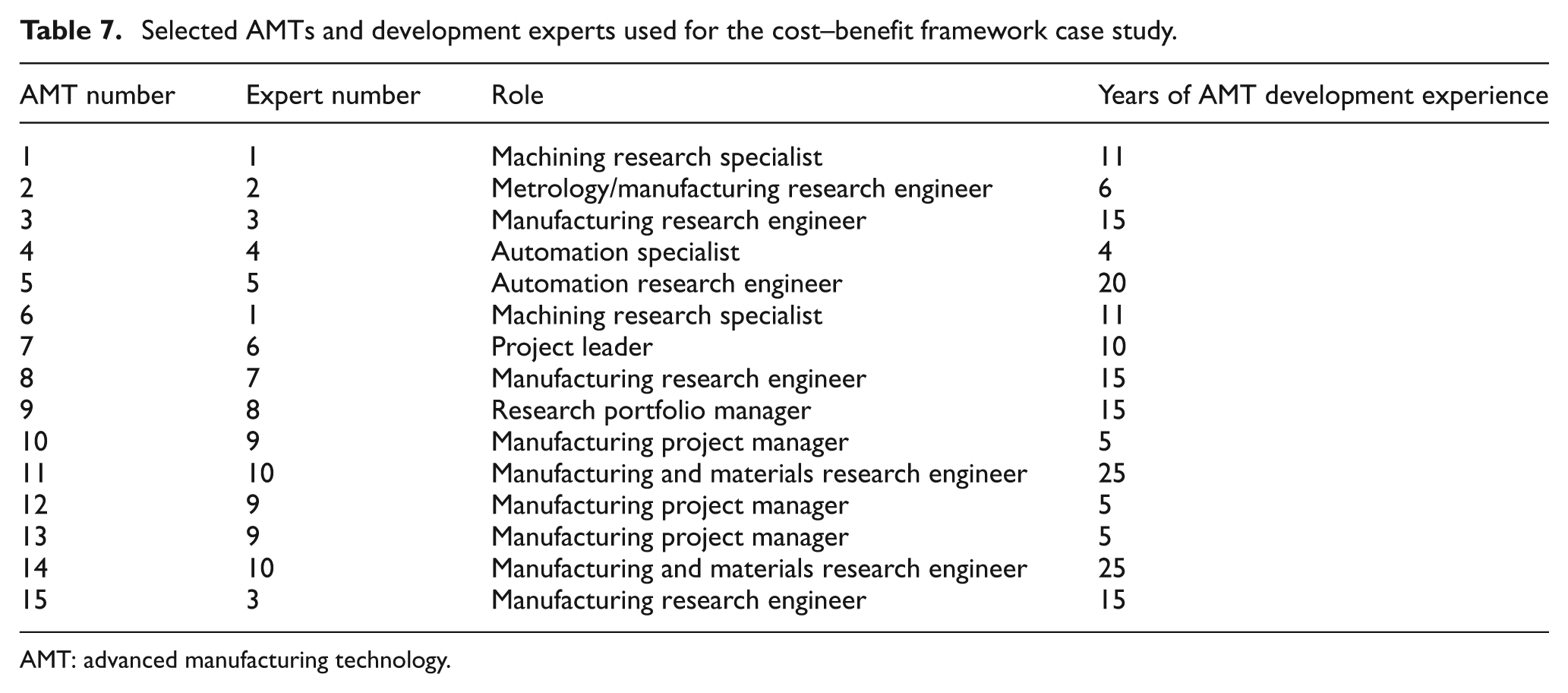
AMT: advanced manufacturing technology.

Stage 1 − user information

The users of the framework are listed in Table 7, with their respective AMT development experience in years and their role within the business.

Stage 2 − AMT identification

The 15 AMTs selected for evaluation within aerospace manufacturing R&T portfolio are numbered in Table 7. Care was taken to capture the most recent TRL reviews for each AMT, certifying that each forecast utilised all available technical information. The 15 aerospace AMTs covered a range of processes and applications, including state of the art in forming techniques, drilling, automation, tooling and machining.

Stage 3A − COTECHMO resources (person-hours) forecast

Stage 3A involved utilising the COTECHMO resources toolset with the mathematical notation explained earlier in section ‘Proposed framework.’ The first step of performing a COTECHMO resource (person-hours) forecast involved capturing data from historical AMT developments to TRL6. Mean TRL6 development data for the 15 AMTs equalled 5374 person-hours. The next step involved calibrating the model size driver, by calculating the mean functional size for the 15 AMTs. The total functional size for the 15 AMTs was 972.5; thus, a mean value was 64.83. Therefore, to equate the output of 5374 person-hours with nominal complexity, the calibration constant was 82.93. This forms the final calibration factor (A) detailed earlier within equation (2).

The next step involved the users operating the Microsoft Excel Resources toolset, with the interface illustrated in Figure 2. Within the interface, cells highlighted yellow require data input. Users counted the functional size requirements and rated the effort drivers for their AMTs. For the intention of this case study, the model was utilised to forecast development person-hours for the 15 AMTs, using the aligned AMT development expert(s) listed in Table 7. The results are presented graphically in subsection ‘Stage 6 − AMT DEVAL evaluation’.

Figure 2.

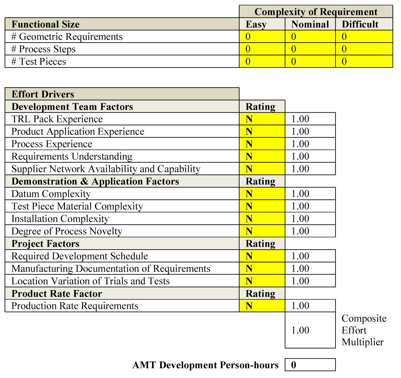
COTECHMO resources Microsoft Excel toolset user interface.

Stage 3B − COTECHMO direct cost forecast

Stage 3B involved utilising the COTECHMO direct cost toolset, with the mathematical notation explained earlier in section ‘Proposed framework.’ The first step involved calibrating the model to historical AMT TRL6 direct cost development data. Mean TRL6 development data for the 15 AMTs equalled €979,942. The next step involved calibrating the model size driver by calculating the mean physical size of the AMT hardware for the 15 AMTs. The total hardware size for the 15 AMT historical cases was 5498.8 m³; thus, a mean value was 366.6 m³. Therefore, to equate the output of €979,942 with nominal complexity, the calibration constant was 2673.4. This forms the final calibration factor (A) presented in equation (4).

The next step involved the users operating the Microsoft Excel Direct Cost toolset, with the interface illustrated in Figure 3 and cells highlighted yellow indicating data input. Users quantified the physical size of the AMT process hardware and rated the cost drivers for their AMTs. Following the resources model, it was utilised to forecast development direct cost for the 15 AMTs, with the aligned AMT development expert(s) listed in Table 7. The results are presented graphically in subsection ‘Stage 6 − AMT DEVAL evaluation’.

Figure 3.

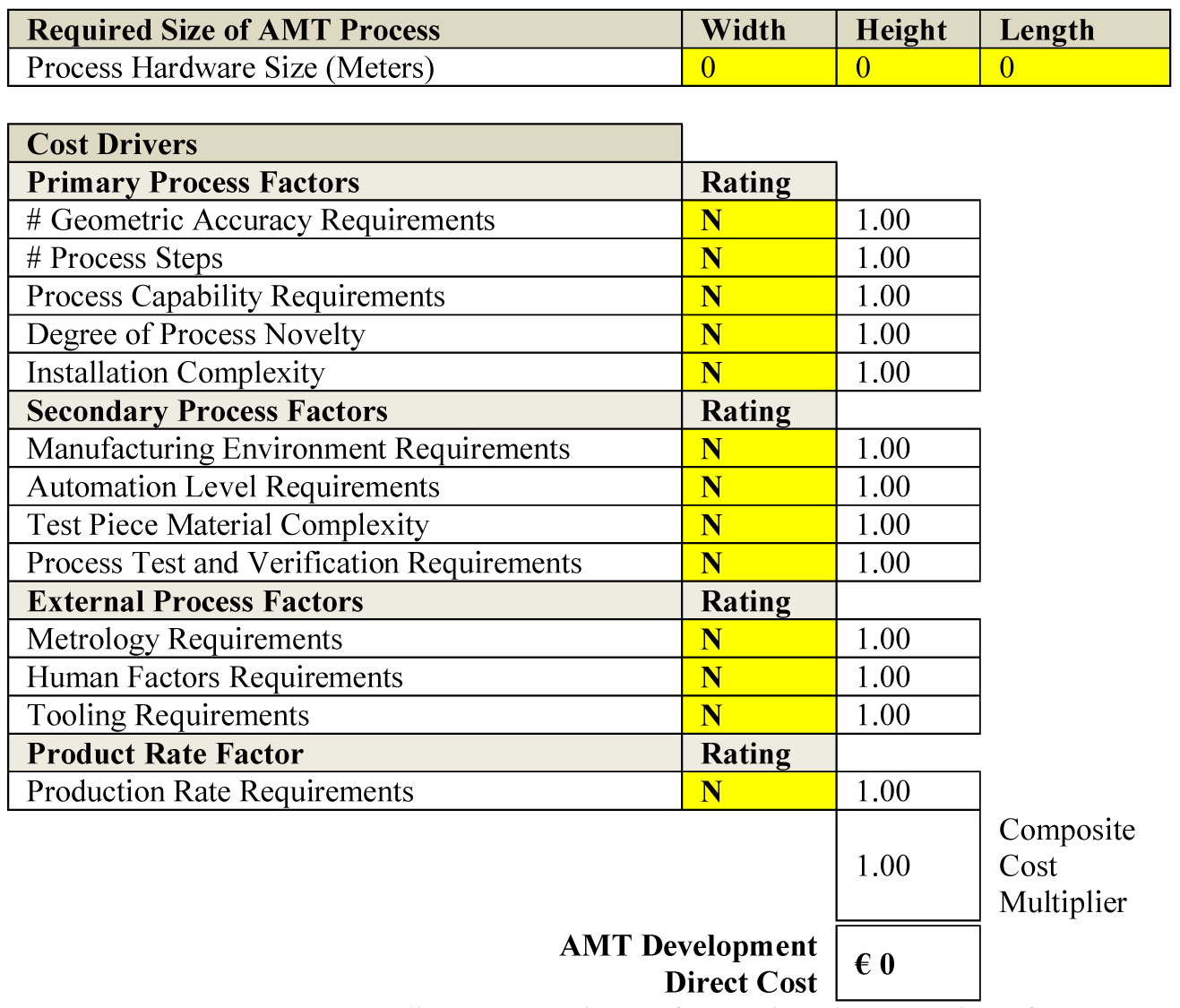
COTECHMO direct cost Microsoft Excel toolset user interface.

Stage 4A − PERFORMO tangible forecast

Stage 4A involved utilising the PERFORMO tangible toolset with the mathematical notation derived in section ‘Proposed framework’ and the Microsoft Excel interface illustrated in Figure 4. Within the interface, cells highlighted yellow require data input. The first step of the performance forecast involved the users weighting each of the 12 KPFs using the definition (judgement) quantitative scale, inputting into the ‘KPF intensity of importance’ column. The next step involved identifying the baseline of the AMT selected for assessment. Model users input the new AMT forecast values from a datum baseline as a three-point estimate using minimum, most likely and maximum change. The toolset was used to perform a tangible performance forecast for each of the AMTs, with the aligned AMT development expert(s) listed in Table 7. The tangible performance output results are presented in subsection ‘Stage 6 − AMT DEVAL evaluation’, with outputs above a value of 1.0 indicating a performance enhancement.

Figure 4.

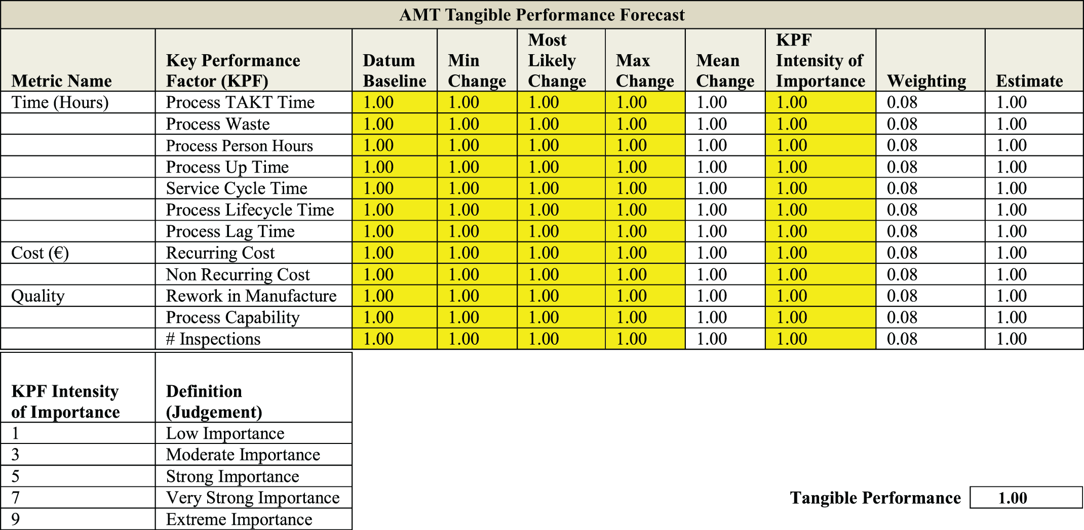
PERFORMO tangible Microsoft Excel toolset user interface.

Stage 4B − PERFORMO intangible forecast

Stage 4B involved utilising the PERFORMO intangible toolset with the mathematical notation presented in section ‘Proposed framework’ and the Microsoft Excel Interface illustrated in Figure 5. Within the interface, cells highlighted yellow require data input. Following the Tangible model process, the first step of performing an intangible forecast involved the users weighting each of the 12 KPFs using the definition (judgement) scale for their AMTs. This quantitative value was input into the ‘KPF intensity of importance’ cells. The next step involved the users rating each KPF. The toolset was used to perform an intangible performance forecast for each AMT with the aligned AMT development expert(s) listed in Table 7. Intangible performance output results are presented in subsection ‘Stage 6 − AMT DEVAL evaluation’, with outputs above a value of 0.0 indicating a performance enhancement.

Figure 5.

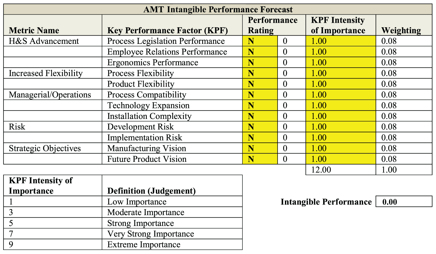
PERFORMO intangible Microsoft Excel toolset user interface.

Stage 5 − DEVAL forecast

On completion of the COTECHMO and PERFORMO forecasting assessments, the data outputs for the 15 AMTs listed in Table 7 were plotted into the DEVAL toolset. The mathematical notation was presented in section ‘Proposed framework.’ DEVAL graphical outputs that follow are detailed with inclusion of development effort and performance thresholds.

Stage 6 − AMT DEVAL evaluation

The final stage of the framework involved assigning development effort and performance thresholds for the DEVAL outputs in Microsoft Excel. Thresholds were assigned with a research manager involved in the overall portfolio evaluation, with 15 years AMT development experience. As part of the AMT evaluation process, the research manager evaluated the results from the 15 AMTs listed in Table 7. The thresholds defined are listed in Table 8, based on the R&T available resources, budget and performance requirements. The final DEVAL graphical outputs are illustrated in Figures 6–9 and were calculated using equations (25)–(28). These DEVAL outputs were then evaluated in detail to select AMTs providing the business with the best value, creating the following results. ‘AMT 4’ was the first AMT recommended for development, despite falling within the upper boundaries of the person-hours and direct cost limits. This AMT was selected, based on its outstanding tangible and intangible performance forecasts. The second AMT recommended for development was ‘AMT 10’. This was selected based on its low forecast development person-hours and direct cost, compiled with tangible and intangible performance forecasts that both fulfilled the threshold requirements. ‘AMT 7’ was considered from the excellent intangible forecast performance; however, from not meeting the tangible performance threshold this AMT was eliminated.

Table 8.

Development forecast thresholds.

Thresholds
Resources (person-hours)	Direct cost (€)	Tangible performance	Intangible performance
8000	1,300,000	2.25	0.30

Figure 6.

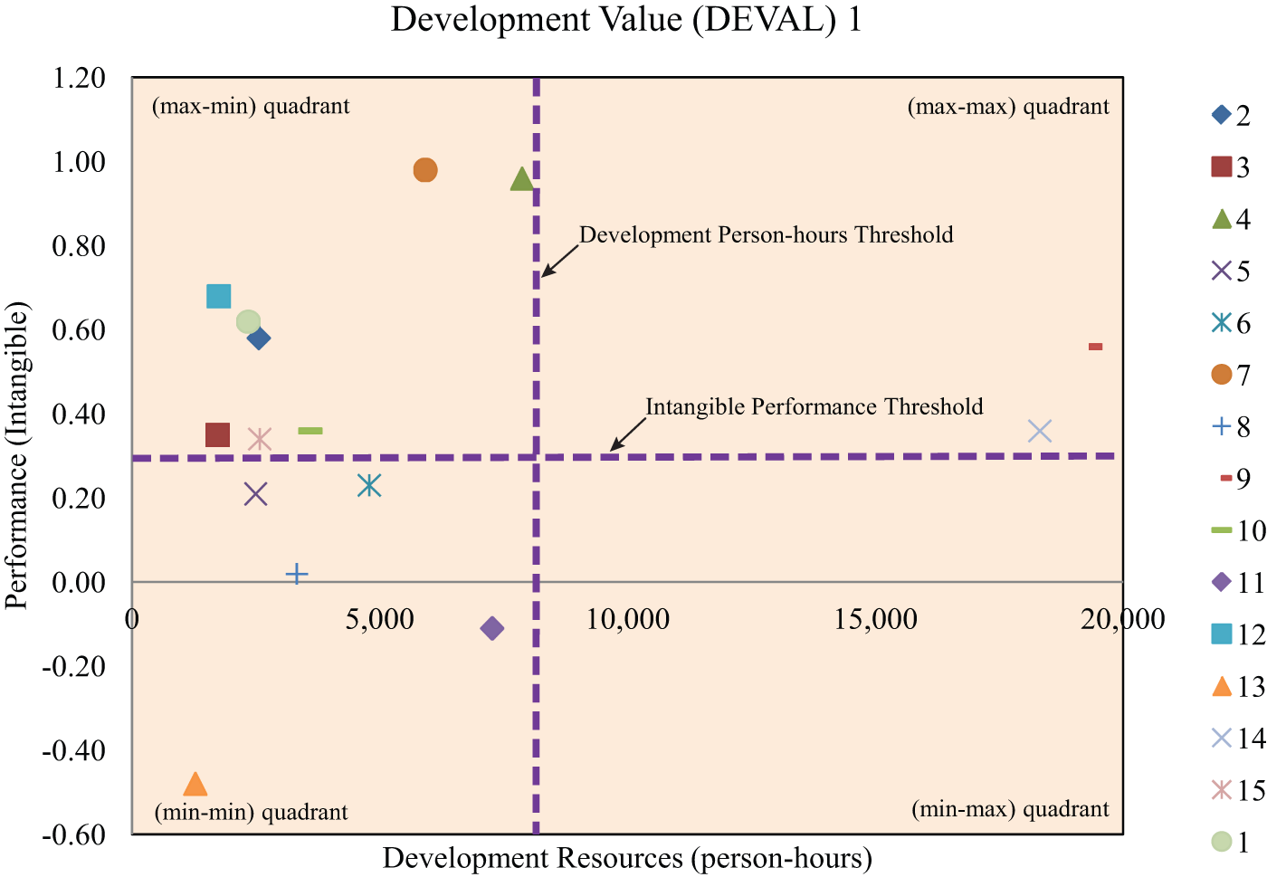
Outputs from COTECHMO resources and PERFORMO intangible models plotted within DEVAL with the assigned thresholds.

Figure 7.

Outputs from COTECHMO resources and PERFORMO tangible models plotted within DEVAL with the assigned thresholds.

Figure 8.

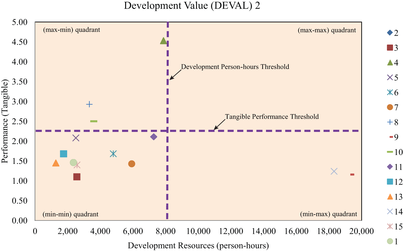
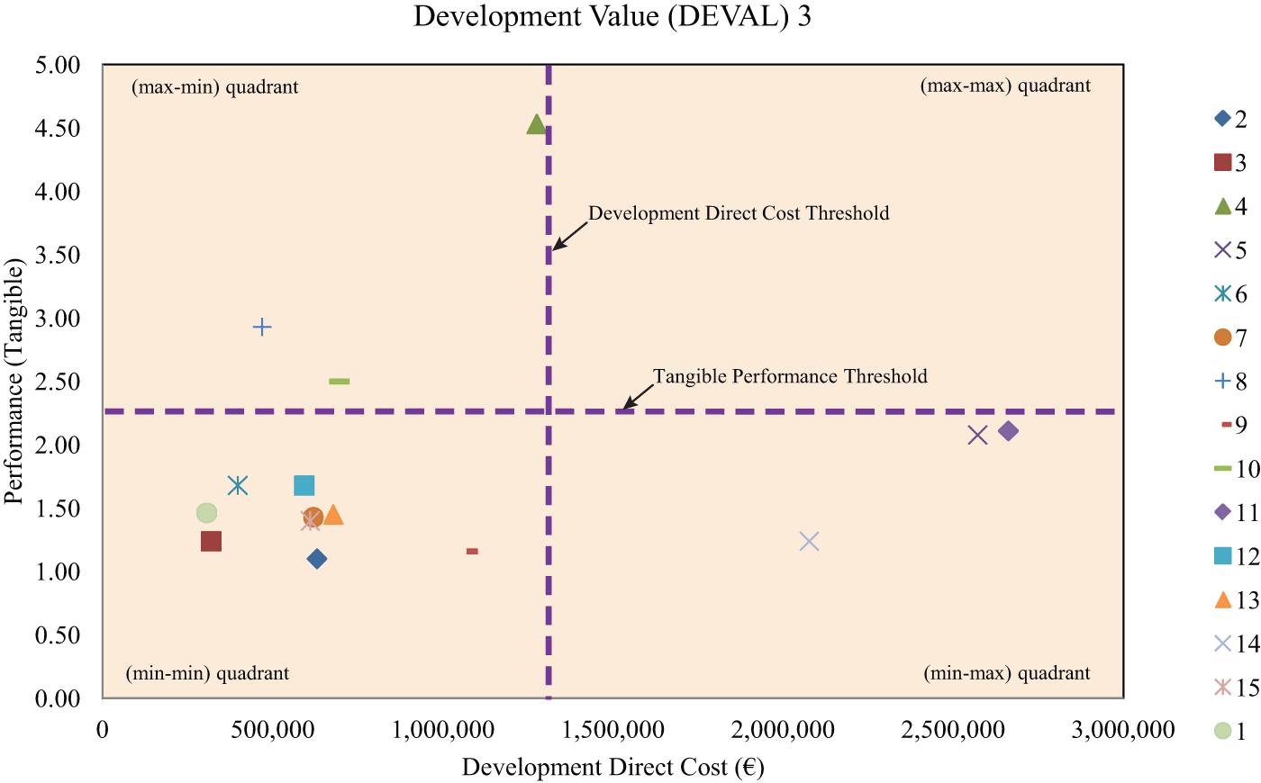
Outputs from COTECHMO direct cost and PERFORMO tangible models plotted within DEVAL with the assigned thresholds.

Figure 9.

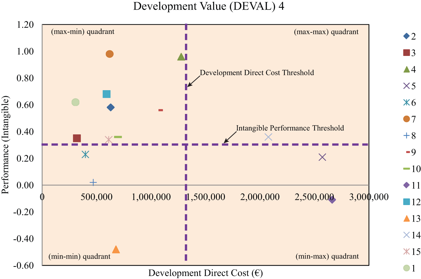
Outputs from COTECHMO direct cost and PERFORMO intangible models plotted within DEVAL with the assigned thresholds.

Framework verification

COTECHMO verification

To perform an initial verification of the COTECHMO resources and direct cost models, the CER forecasting accuracy of each was tested using ‘Prediction Level’ (PRED) values. The industrial specification required the data to fall within PRED(20). A PRED(20) value specifies the forecast data to fall within 20% of the actual value.^12,26 For the purpose of this case study, the forecast is compared to the actual development value of the AMTs listed in Table 7. To calculate the PRED value, the number of forecast cases falling within 20% of the actual data is divided by the total number of cases. On review of the COTECHMO resources model CER forecasting accuracy, 53% of the data fell within PRED(20), 73% within PRED(25) and 86% within PRED(30). The COTECHMO direct cost model forecasting accuracy was higher than the resources model, with 93% of the development data falling within PRED(20) and 100% falling within PRED(25). Further verification was provided by multiple regression analysis on each COTECHMO model using the 15 AMT case studies. Within this analysis, a model significance F-test was performed to identify the statistical significance of each model hypothesis. The resources model had an outstanding F-value of 106.65, verifying the model hypothesis. The F-value for the direct cost model was lower at 5.59, although this was still sufficient to verify the model hypothesis. To provide further verification, an R-squared value for each model was calculated. The resources model produced a high value of 98% and the direct cost model a value of 76%, with each verifying the models statistical significance. Further details of each COTECHMO model verification including a detailed driver sensitivity analysis using t-values and p-values can be found within the paper from Jones et al. ²⁷

PERFORMO verification

To verify the PERFORMO tangible and intangible models, AMTs with known conclusions were selected. The 15 AMTs numbered in Table 7 were not fully developed and implemented within manufacturing operations. Therefore, eight AMTs with known conclusions were selected, five had been successfully implemented within manufacturing operations and three were unsuccessful. The five successful AMTs were ranked based on their actual data within operations. The PERFORMO tangible and intangible models were then used to forecast the performance. These forecast performance outputs were checked for correlation with the ranking from the actual operations data. The output ranking was coherent for four of the five AMTs for the tangible and intangible models, equating to an accuracy of 80%. Three AMTs determined unsuccessful were also checked using each model. Each model predicted all three of the AMTs unsuccessful, verifying model accuracy. However, the intangible model predicted one of the three unsuccessful AMTs with a performance value of −0.02. This value was only 0.02 away from the model becoming inaccurate and determining an incorrect decision, with an output above 0.00 defining a successful AMT. The minor discrepancies in each model are the subject of future research recommendations, discussed within section ‘Conclusion’.

Framework validation

The statistical verification discussed previously is a quantitative form of validation. To further validate within an industrial setting, a questionnaire was developed. The questionnaire used three applicability criteria proposed by Platts and Gregory. ²⁸ This was successfully utilised by Evans et al. ²³ within the manufacturing domain including feasibility, usability and utility. Feasibility defines if users can follow the methodology, usability determines if it is easily followed and utility studies the output. Table 9 lists the final criteria of the questionnaire, showing the segmentation of each under the applicability criteria discussed. The experts listed in Table 7 were asked to fill in the questionnaire after using the framework and rate each question using the ‘Likert scale’. Results of the questionnaire are presented graphically in Figure 10, with the question numbers on the ‘x-axis’ and the average rating from the 10 users on the ‘y-axis’. On detailed evaluation of the responses, every question, excluding question 2.5, averaged above a value of 4, indicating that each of the experts agreed with the framework. Question 2.5 scored below a value of 4, with a value of 3.5 and when scrutinised with experts, many rated the data input of the framework ‘neutral’ from difficulties calibrating each forecasting model. Nonetheless, each agreed the framework calibration user complexity would reduce if they were to utilise the framework again.

Table 9.

Cost–benefit framework validation questionnaire.

Assessment criteria	1	2	3	4	5
1. Feasibility
1.1. Framework is logical for forecasting AMT development value?
1.2. Framework is suitable for forecasting at the initial development stages?
1.3. Time taken to perform a cost–benefit forecast was appropriate?
1.4. Framework enhances existing AMT cost–benefit forecasting techniques?
2. Usability
2.1. Objective and purpose of using the framework was clearly defined?
2.2. Framework interfaces were easy to use?
2.3. Stages of the framework were easy to follow?
2.4. Framework software was intuitive?
2.5. Data input can be performed easily?
3. Utility
3.1. Framework cost–benefit analysis had the appropriate level of granularity?
3.2. Framework stages were in the correct order?
3.3. Final value output was correct for your AMT?
3.4. Framework final output was appropriate for its application?
4. Suggestions
4.1. Strengths of the framework
4.2. Weaknesses of the framework
4.3. Areas for improvement

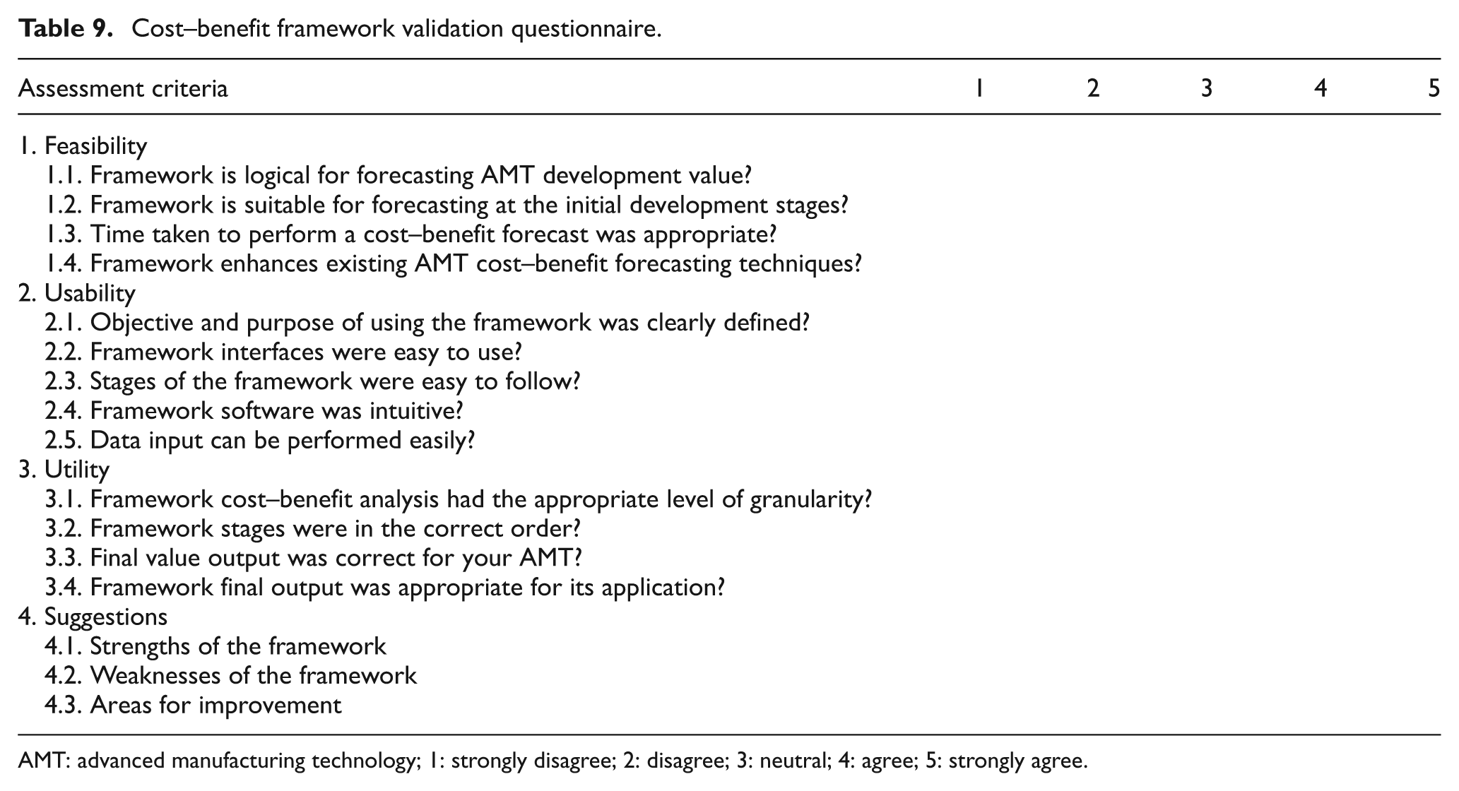
AMT: advanced manufacturing technology; 1: strongly disagree; 2: disagree; 3: neutral; 4: agree; 5: strongly agree.

Figure 10.

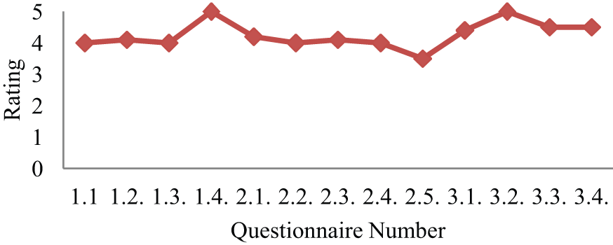
Average questionnaire ratings from 10 AMT development experts.

Conclusion

At present, there is no existing framework capable of forecasting the cost–benefit of AMTs at the initial stages of development. The research presented has successfully developed a novel cost–benefit framework for aerospace AMT development. The framework has been statistically verified using 15 AMTs for each COTECHMO model and 8 AMTs for each PERFORMO model.

Ten AMT experts have successfully validated the framework within an industrial application. Within this analysis, experts identified many significant strengths of the framework. A primary strength was the suitability of the outputs from COTECHMO and PERFORMO, providing DEVAL at the initial stages of development. Additionally, experts defined the TRL as a faultless platform to perform the cost–benefit assessment within manufacturing R&T. Experts were also impressed by the framework capability to reduce AMT development risk, by constructively quantifying KPFs at the early development stages. This was enhanced within the PERFORMO tangible model, from inclusion of performance forecasting uncertainty, using a three-point estimate. Generally speaking, experts were impressed with the framework capability to enhance existing R&T investment decision-making for AMT development.

Despite these significant strengths, there were some minor aspects of the framework identified for enhancement. The first suggestion involved linking each of the stages and models seamlessly within Microsoft Excel, using Visual Basic for Applications, creating a more robust framework. This would enhance the operation of the forecasting models and each framework stage, guiding the user and the data required. Alignment to the overall project and programme management software used within aerospace R&T was another suggestion. Experts identified that implementation of the framework would enhance existing planning software in a constructive manner.

The presented cost–benefit framework has been successfully verified and validated within a large aerospace manufacturing organisation. To further verify each COTECHMO and PERFORMO model, additional AMTs with known outcomes could be selected and evaluated. Future research could also implement the framework into other aerospace manufacturing organisations. In this instance, each forecasting model within the framework would require statistical calibration. This would further support the overall framework methodology and extend the impact outside the supporting organisation.