Sage Journals: Discover world-class research

Abstract

Designing parts with freeform surfaces, as typically applied in dies and moulds, is currently dealt with through designer experience, if design intent is to be maintained and if, at the same time, the manufacturing process is to be facilitated. This work puts forward a solution to these issues which is based on computational intelligence. A library of freeform surface morphological features is defined using parametric wireframe models that include constraints. The part is constructed using wireframe features from this library and these are subsequently converted to solid models. The effect of changes of feature parameter values is linked to part functional characteristics in standard design environment. Regarding the effect on manufacturing process characteristics, various models may be employed. As an example, a fuzzy system that decides tool diameter and the necessity of a semi-finishing operation is employed in this work. Artificial neural networks are trained with a number of workpiece variations corresponding to different feature parameter values and the pertinent outputs from functional and manufacturing assessment. Next, a standard genetic algorithm is set up to find the best values of the feature parameters based on both functionality and manufacturing criteria with suitable weighing. The evaluation function of the genetic algorithm employs the artificial neural networks constructed as metamodels. The methodology is demonstrated through an illustrative case study, but may encompass further Design-for-X disciplines.

Keywords

Freeform surfaces design optimisation design for manufacturing neural networks genetic algorithms

Introduction

The shape of a mechanical engineering part needs to satisfy a multitude of requirements: function, strength (against mechanical loads, thermal loads, etc.) and, in addition, in a Design-for-X (DfX) context further requirements.¹ For instance, in a Design-for-Manufacturing (DfM) context, manufacturability is required, denoting ease and cost of manufacture; in a Design-for-Assembly (DfA) context, assemblability is sought, denoting ease and cost of assembly and similarly in other contexts within Product Lifecycle Management (PLM), for example, Design-for-Maintenance and Design-for-Recycling. This work focuses on DfM as a representative example of PLM domains contributing to multi-disciplinary design optimisation (MDO), but without loss of generality.

Taking into account at the design stage, all pertinent requirements are a matter of optimisation because of their sheer number and often contradictory nature. Each requirement is associated with one or more assessment criteria and pertinent constraints. Typically, the designer does not solve this optimisation problem in an orthodox mode (forward or inverse) but, instead, makes choices based on experience, intuition and rough calculation and then checks the result against assessment criteria and constraints using design and analysis software tools. In any case, the design process advances through trial-and-error cycles, experimentation being facilitated by the part model being expressed in some parametric form. However, in the case of freeform surface parts, commercially available tools support parameterisation at the level of the surfaces as such, rather than at the feature level.

With a view to setting up and supporting the optimisation process on a software platform, three issues arise: (a) representing the part shape in an appropriate way, (b) defining and representing assessment criteria to support designer’s intent and intuition and (c) adopting suitable optimisation techniques in order to reach solutions in a realistic time framework.

Let it be clear from the onset that the state of the art in mechanical design optimisation is limited to quantification of an initial design that has been already established qualitatively by a human creativity process, which is so far poorly understood in the field of the cognition science.²

As far as the first issue stated is concerned, part variant representation may be driven by design tables especially for two-dimensional (2D) profiles.³ Parametric curve and surface representation linked to some form of deformation energy that needs to be optimised are also possible alternatives.⁴ Yet another possibility is offered by expressing the shape at hand as a combination of a small number of basic shapes and relevant weights, both of which are to be determined through optimisation.⁵ In the case of full three-dimensional (3D) parts, however, feature-based shape representation is the most significant contender, a prime reason being that this is the standard paradigm of current computer-aided design (CAD) systems. Freeform surface features are both mathematically and notionally more intricate than classic features.⁶ Features are defined as templates in libraries and are then recalled, instanced, that is, their parameters are assigned values, and inserted into the part being designed, that is, reused,⁷ the main issue being the way in which features are fitted into the existing model, thereby interacting with the other features.⁸

In this work, among the various categorisation schemes concerning freeform surface features, semi-free features are adopted, as defined through classic operators (sweep, loft, etc.), interpolation and functions operating on curve/surface control points. In addition, van den Berg’s suggestion is adopted, too, whereby feature internal characteristic points related to 2D profiles that are used in feature definition are mapped to boundary freeform surfaces together with distance, angle, position and validity (dimension, curvature, interaction and continuity) constraints.^9,10

As far as the second issue is concerned, in the vast majority of cases, part shape constrained optimisation employs structural criteria leading to optimisation of mass distribution and/or topology,¹¹ whereby some constraints may stem from manufacturability/assemblability considerations.⁴ There are very few references alluding to the need to integrate into MDO manufacturing, let alone manufacturing cost.² Optimisation may involve capturing manufacturing knowledge as rules linked to design validation and be implemented into a web-based PLM prototype.¹² Manufacturing cost may be minimised subject to structural performance limits. For every design iteration, structural performance is evaluated by finite element analysis (FEA), and machining time and cost are estimated by virtual machining (computer-aided manufacturing (CAM)).¹³ Manufacturing considerations inevitably pass through process planning, especially rough cut, the pertinent digital tools (mostly based on fuzzy logic) being sparse, examples concerning evaluation of machinability^14,15 and forgeability.¹⁶

In this work, it is recognised that an array of software tools and techniques support design verification and validation, be it engineering,¹⁷ manufacturability analysis¹⁸ or downstream product life-cycle stages.¹⁹ Thus, it is advocated that most of these tools do enable construction of metamodels for assessing design solutions in place of these very tools.

As far as the third issue is concerned, suitable optimisation techniques are well documented in literature.⁴ Classic methods such as gradient-based, variational methods and linear programming are certainly a choice, especially in the presence of only few control parameters.²⁰ Furthermore, stochastic/probabilistic design optimisation is well established by perturbing design parameter values and capturing statistically the effect on the cost function.³ However, evolutionary methods are much more popular in recent years, not only in shape and topology domain²¹ but foremost in multi-parameter, multi-objective and, more recently, multi-disciplinary optimisation where the solution hypersurface has a number of local extrema. The stochastic nature of such methods enables them to explore large solution spaces fast and makes them immune to discontinuities, convexity issues and noise. Comprehensive application examples in shape optimisation are given by Roy et al.⁴

Interesting tools supporting evaluation through meta- or surrogate models, multi-objective evaluation and Pareto fronts have been reported.²² Response surfaces are simple and effective metamodels when the number of design variables is typically less than 10²³ and can guide optimisation by adaptive screening of regions of interest, for example, in metal forming die optimisation to minimise its stresses.²⁴ Neural networks (e.g. radial basis function (RBF)) are also used as metamodels, when the number of design variables is large²³ or when computationally inexpensive rough evaluation of solutions is necessary. MDO optimisation is a relatively recent development enabled by increasing computational power available. Surrogate models have a special role in this paradigm.²⁵ MDO methods accounting for natural changes in user requirements over time have recently been reported enabling moving from one design on the Pareto frontier to another.²⁶

In this article, genetic algorithms (GAs) are used to implement multi-disciplinary optimisation. Multi-disciplinarity involves manufacturing issues alongside functional design issues. All assessment/engineering simulation tools are replaced by artificial neural network (ANN) metamodels that are precisely trained using a restricted number of data. The overall concept is shown in Figure 1.

Figure 1.

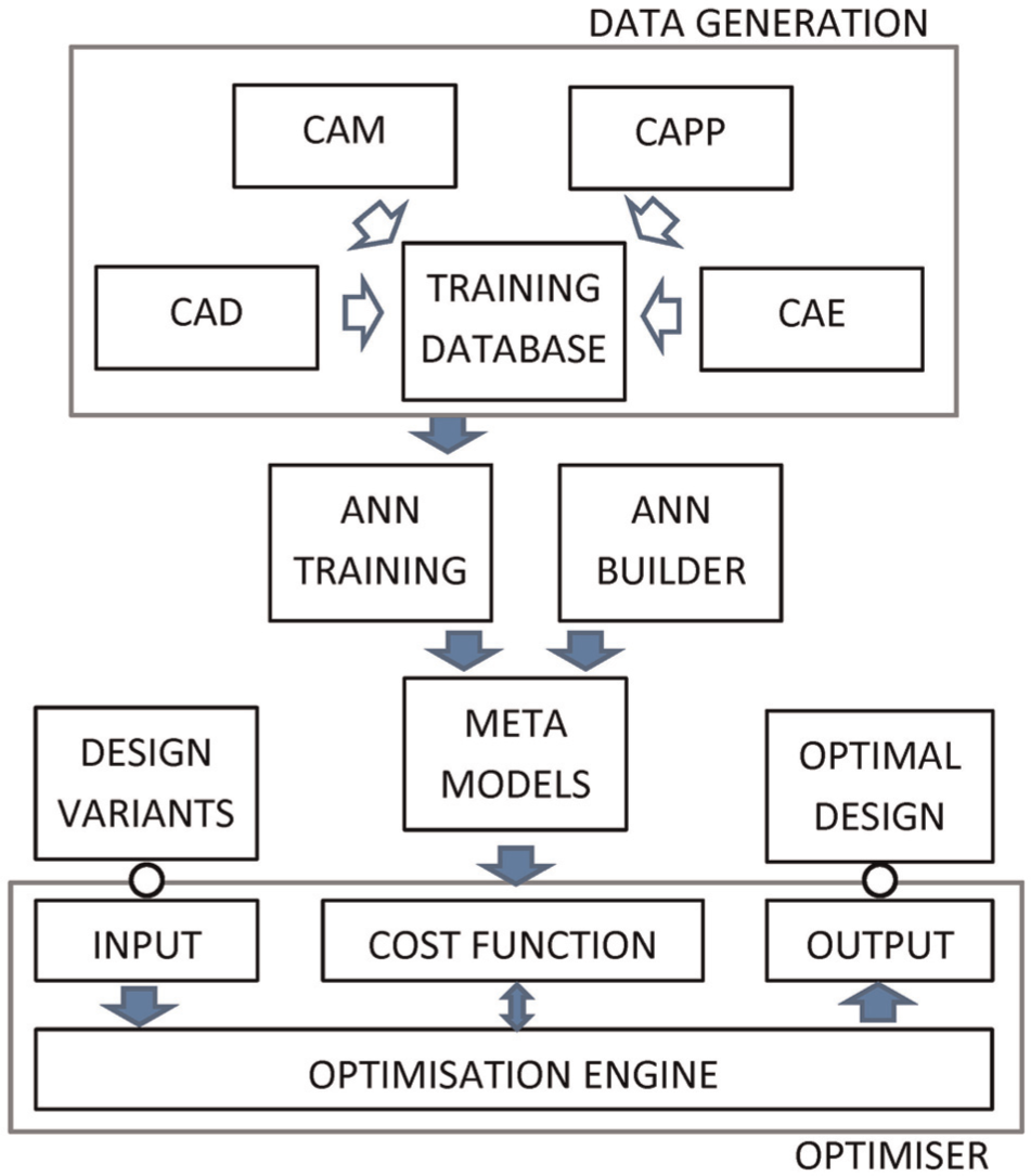
Overall system concept.

The novelty of this work consists in the following: (a) manipulating part shape expressed by a novel freeform surface feature representation, which has not been reported on in the literature so far; (b) demonstrating consideration of manufacturing criteria, which is rare indeed in MDO and (c) homogenising the assessment of all constituent parts of the GA fitness function through ANN metamodels. Use of metamodels has been reported on a lot in the literature, but in this case, their performance is guaranteed since they are constructed by special custom-developed software. Section ‘Parametric design of freeform surface parts’ presents parametric design of freeform surface parts by features. Optimisation parameters and criteria are discussed in section ‘Modelling and optimisation’. Section ‘Metamodel creation’ outlines the development of metamodels and sections ‘Design optimiser’ and ‘Results and discussion’ present the GA employed for optimisation purposes and typical results obtained, respectively. Conclusions are laid out in section ‘Conclusion’.

Parametric design of freeform surface parts

A constraint and feature-based paradigm of parametric design is adopted, which enables a topology-based representation of the part, thereby safeguarding the design intent and at the same time facilitates generation of variants.

Notions

A freeform surface feature is defined by curves (profiles), that is, by a wireframe model (see Figure 2(a)).

Figure 2.

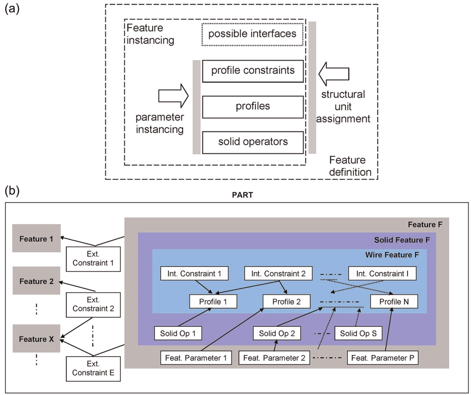
Freeform surface feature notions: (a) feature definition and (b) part definition.

The profiles are determined by parametric dimensions and internal constraints. These refer strictly to curves and not to surfaces or solids. Constraints may be purely dimensional or geometric. The latter concern collinearity, tangentiality, perpendicularity, fixed location, parallelism, concentricity and so on as commonly found in all major modern CAD systems. Profiles may be defined also as interfaces of the respective feature to other features, in which case the corresponding constraints are termed external.

The corresponding solid model feature is generated by applying the appropriate operators, typically: extrusion, rotation, sweep and loft. Parametric representation is applicable overall to profiles, constraints and operators. Assigning values to these parameters results in feature instancing and variant generation. In the framework of feature definition, it is possible to use alternatively different profiles, different constraints for the same profiles and different interfaces.

Features may be classified as primary and secondary. Each part consists of at least one primary feature. Features may also be classified according to the solid modelling operator that is required to generate its model, that is, extruded, revolved, swept and lofted. Secondary features are also classified according to the way in which they are combined with the existing features to build the part model, namely, union, subtraction and intersection (see Figure 2(b)).

A feature may also be classified according to its functional role in the design. The more general this function, the feature shape requirements and its relationship to other features, the larger the probability of its use in different part classes or families.

External constraints are generally required in order to define and control feature interactions in the part. Therefore, the designer must have a general idea on how the features are to be combined into a part in order to apply such constraints; catering for the general case is obviously meaningless. External constraints may be expressed as inequalities linking dimensions of two or more features. Thus, their validity can only be checked at feature instancing. External constraints may also be of geometric nature, in which case they are necessary not to check validity of the part but to build the part as such. However general they might appear to be, external constraints are certainly difficult to standardise and are often possible to satisfy only by modifying the individual features to which they apply.

Example

A hammer is designed by using four features defined in Table 1. Special attention is to be given to the control parameters that enable each feature to be defined in a compact way. The solid model shape, its corresponding wireframe sketch and the control parameters are depicted in Figure 3.

Table 1.

Definition of four features combined in hammer design.

Name	Functional specifications	Construction class	Building class	Control parameters	Internal constraints
Claw	Wedge/lever shape	Extrusion	Addition	2	11
	Compact, concentrated mass			Width a (2α)
	Large interface profiles			Depth b
Head	Extension feature	Rotation	Addition	2	17
	Axisymmetric			Height c
	Large flat end			Width d
Tang	Bridging/extension feature	Loft	Addition	2	12
	Longitudinal shape			Length e
	Planar symmetry			Thickness f
Handle	Bridging/extension feature	Rotation	Addition	2	12
	Longitudinal shape			Length g
	Human hand compatibility			Thickness h

Figure 3.

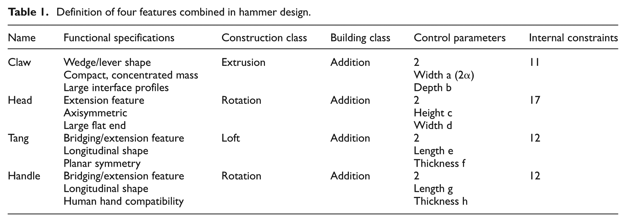
Features: (a) claw, (b) head, (c) tang and (d) handle.

Furthermore, details are given regarding the feature claw as an example. The planar profile used for claw feature construction is composed of two circles of radii α and α/3, respectively; their centres being placed on the endpoints of a line of length 10α/3. Two arcs of radii 4 ×ακαι (8/3) ×α are, then, drawn tangentially to the two circles (see Figure 3(a)). The circles are trimmed to the arc ends. There are five dimensional constraints and another six geometric constraints (tangentiality and circle centre location). The control parameters are the radius α and the depth (thickness) of the claw (b). Internal constraints consist also of an equation relating the two control parameters to ensure required proportions: b ≥ 1.35*α. Extrusion and subsequent filleting result in the solid model of the claw feature.

Various hammer models and the corresponding forging dies as their negative volume counterparts can be defined by exploiting the presented features (see Figure 4). The model is validated essentially by the application of external constraints.

Figure 4.

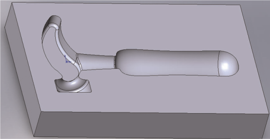
Indicative feature-based hammer die.

Discussion

Freeform surface features for mechanical engineering parts are dealt with as semi-free shapes.⁹ They are defined as fundamentally wireframe features, which are straightforward in the current constraint-based design systems and are subsequently turned into solids by appropriate operators. This approach does not work for non-volumetric features, for which the – almost natural – tendency of the designer to split the part into separate volumes does not apply, which is the case with stylistic or aesthetic design.⁹

Generation of part variants of a strictly defined family based on a clear-cut order of design steps embedding external constraints between features does safeguard design intent by keeping feature validity through these steps. Volumetric features with freeform surfaces can function very well in such a well-defined environment. However, in the framework of a looser process, where feature input order is left unspecified and external constraints are instanced after feature input into the part, design intent is possible to violate, at least given the current design constraint management state of the art.

Modelling and optimisation

Evaluation criteria

From the multitude of quantities that relate to the desirable function of the designed part and to the ease, or equivalently, the generalised cost of manufacturing the part, some indicative ones are presented next to serve as an example of the methodology advocated without loss of generality.

As a principle, it is stated that all variations in shape of the designed part are achieved through a change in values of the control parameters of the features of which it is composed, under the respective constraints, of course.

Examples of quantities that are considered necessary for evaluating design solutions in the optimisation framework presented are given next.

Functional criteria

During mechanical part design, there are often functional requirements that refer to part size. By varying some dimensions of the part, the designer also usually varies the total volume, the total area of the part and so on which are significant functional quantities, yet not primary but derived. Often the difference of the volume, area and so on from respective targeted values is an evaluation criterion. In addition, part size may be required to belong to a range of values, but this is achieved by several combinations of values of the control parameters of the part features. In the hammer example, the volume and surface area of the part (or half of them if the corresponding forging die is considered) are calculated directly by the CAD system.

A particular category of functional requirements is the characteristic distances of part elements, a typical case being the distance of the centre of mass from specific functional axes or specific functional points. For example, in the particular part examined here, the distance of the hammer’s centre of mass from the axis of its handle feature (Yc) is focused on and may need to be small enough to justify a balanced part (see Figure 5). Another example is the distance between the projection of the hammer’s centre of mass on the handle axis and the centre of the handle (Xc). The hammer’s impact force increases with this distance (see Figure 5). These distances are straightforward to calculate from the CAD model.

Figure 5.

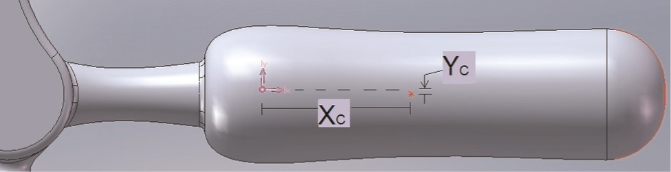
Functional characteristics.

Manufacturing criteria

The designed part can be machined as such or a die can be machined to mass produce this part via forging, casting and so on.

In the case of die milling, several manufacturing criteria can be employed, namely, machining time, surface quality or even strategy indices such as suggested cutting tool diameter. Combinations of parameters can also be used as indicative of results, such as the ratio of material removal volume to roughing tool diameter which can be used as an index for roughing time, the ratio of final surface area to finishing/semi-finishing tool diameter that can be used as an index for finishing time and so on.

As an example, for the particular case examined, the diameters of rough milling tool (D_R) and those of finishing tool (D_F) are selected under the assumption that semi-finishing is always required. These values are determined according to a decision support system that is briefly presented next. Note that milling strategy parameters were ignored since these were determined so that the particular cutting tools achieve a predetermined ratio of machining time to achieved surface quality, which, once decided, is considered to remain constant.²⁷

The selection of appropriate milling tool diameter and cutting strategies for the production of dies is a multi-parametric problem. This is usually dealt with using simulation runs on CAM software but can be automated by a fuzzy system. Such a system is described in detail in Giannakakis et al.²⁷ comprising six fuzzy modules implemented on MATLAB. The modules refer to selection of roughing tool diameter, selection of finishing tool diameter, need for a semi-finishing phase, and selection of cutting strategy for the three corresponding phases.

The input parameters and their membership functions were introduced and created based on data from industrial partners, while the correlation of parameters used for the creation of fuzzy rules was based on CAM simulation results.

Roughing tool diameter selection needs the total volume to be removed and the final-to-initial surface ratio (FISR), which is taken to represent the complexity of the die surface. The term initial surface implies the projection of the final die surface to a plane perpendicular to the tool axis. The larger the total volume to be removed from the die block, the larger the roughing tool diameter to be selected. On the other hand, the higher the FISR, the smaller the roughing tool diameter selected. The module is shown in Figure 6(a), including pertinent membership functions. Note that the result rarely coincides precisely with a diameter that is actually available in the tool library, thus the closest approximation should be selected. Sample rules read, ‘If TotalVolume is VeryLarge and FISR is Small then RoughTool Dia is VeryLarge’.

Figure 6.

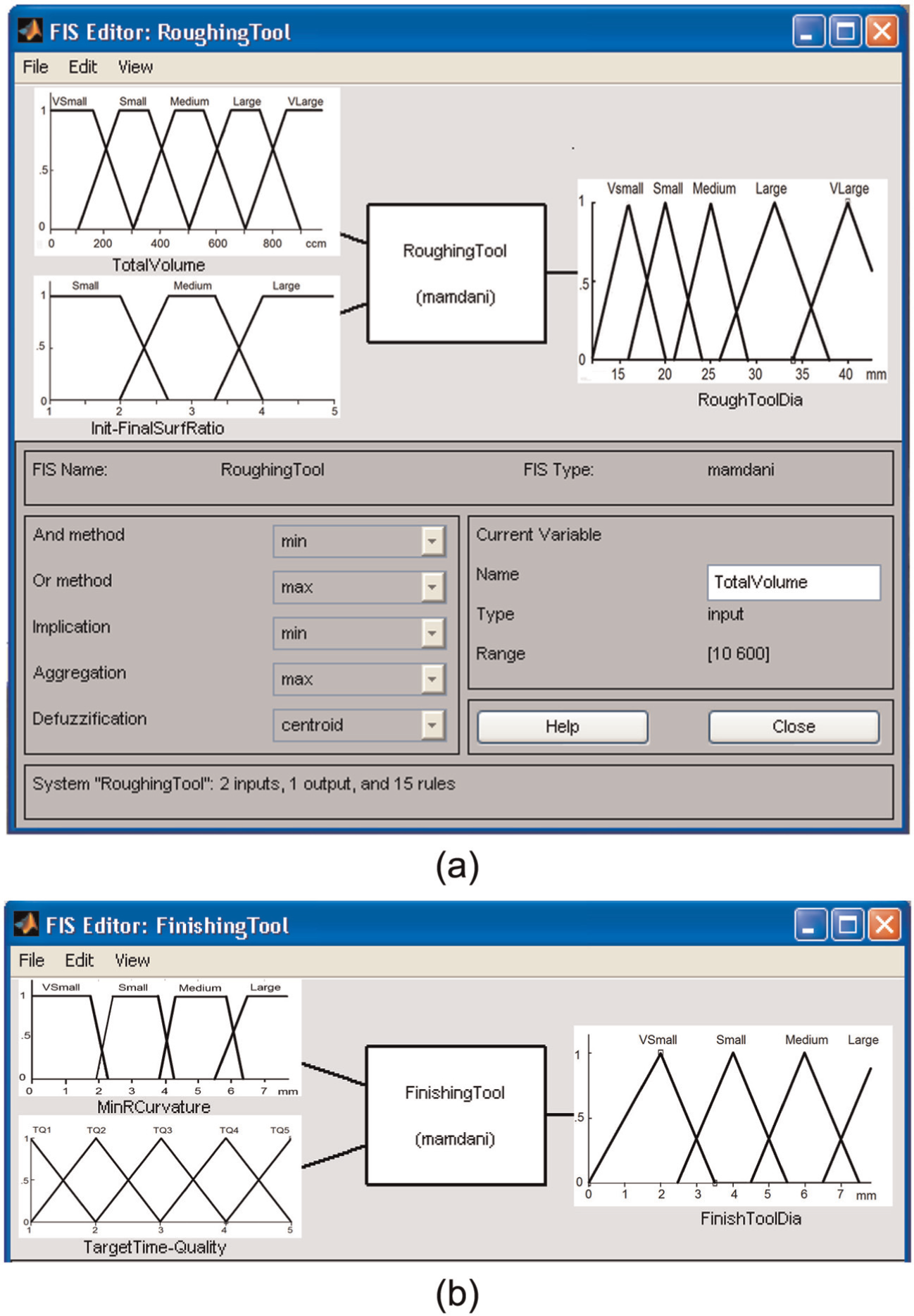
Fuzzy tool diameter selection system outline: (a) roughing and (b) finishing.

Selection of the appropriate diameter of a ball-end finishing/semi-finishing tool depends on the minimum radius of curvature and the time-quality criterion (see Figure 6(b)). Decisions concerning finish machining of the die might tend towards minimisation of time (level 1) or maximisation of quality (level 5), these two objectives imposing contradictory requirements. The user should decide on the value of the time-quality criterion and keep this constant throughout. In total, 20 fuzzy rules result from combining four levels of minimum radius of curvature and five levels of time-quality criterion.

Metamodel creation

ANNs

ANNs are particularly suited to engineering problems that are difficult to model and/or hard to solve analytically or numerically. The particular ANNs of the supervised learning type, and more specifically multi-layer perceptrons,²⁸ aim to code effectively cause–result relationships underlying the problem by pertinent examples acquired through experiments or simulations. Thus, an advantage of ANNs is that there is no need to explicitly model the problem under study. Having learned from these examples, the ANN can respond correctly not only within the same numerical domain (memorisation) but also for similar but not identical cases (generalisation). This is another advantage of ANNs over statistical techniques.

An ANN processes numerical data in multiple units called neurons. Data are passed to them through synapses or connection links, each one having an associated weight (w). Each weighted input (p) reaching a neuron is summed up with the others and constitutes the input to the so-called activation function (ϕ) that is usually universally applicable to all neurons. The result (y) constitutes the response of the neuron (see Figure 7(a)).

Figure 7.

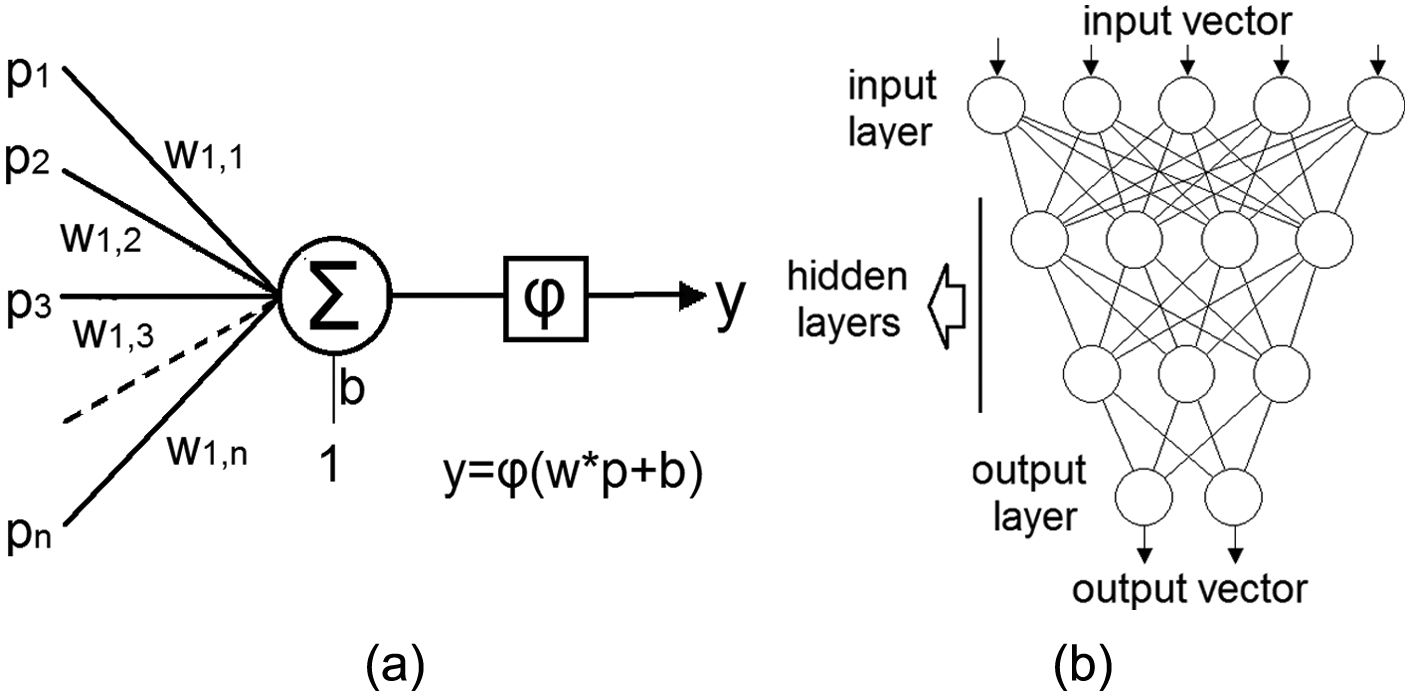
(a) Neuron computations and (b) ANN.

The architecture of the ANN, that is, number of neurons and number of layers beside input and output layers (see Figure 7(b)), as well as the activation function is often decided by trial and error. However, there are also specific algorithms that seek to optimise ANN architecture given a number of training vectors.²⁹ The way in which weights are determined is a matter of the training algorithm, the aim being to minimise the difference between the training example outputs and the response of the output neurons. This is the almost standard ‘feed forward back propagation (of the error)’ training algorithm. Its inherent slow training speed is counterbalanced by alternative variations, notably, momentum-based, adaptive rate, resilient and Levenberg–Marquardt variations.²⁸

ANN training database creation

Enough data for ANN training have to be generated in the framework of the optimisation quantities drawn up. Essentially, the values of feature control parameters have to be changed to generate corresponding variants of the design, and the corresponding values of optimisation criteria have to be obtained either directly from the CAD system (regarding functional criteria) or indirectly by executing the appropriate manufacturing-related simulation program (regarding manufacturing criteria).

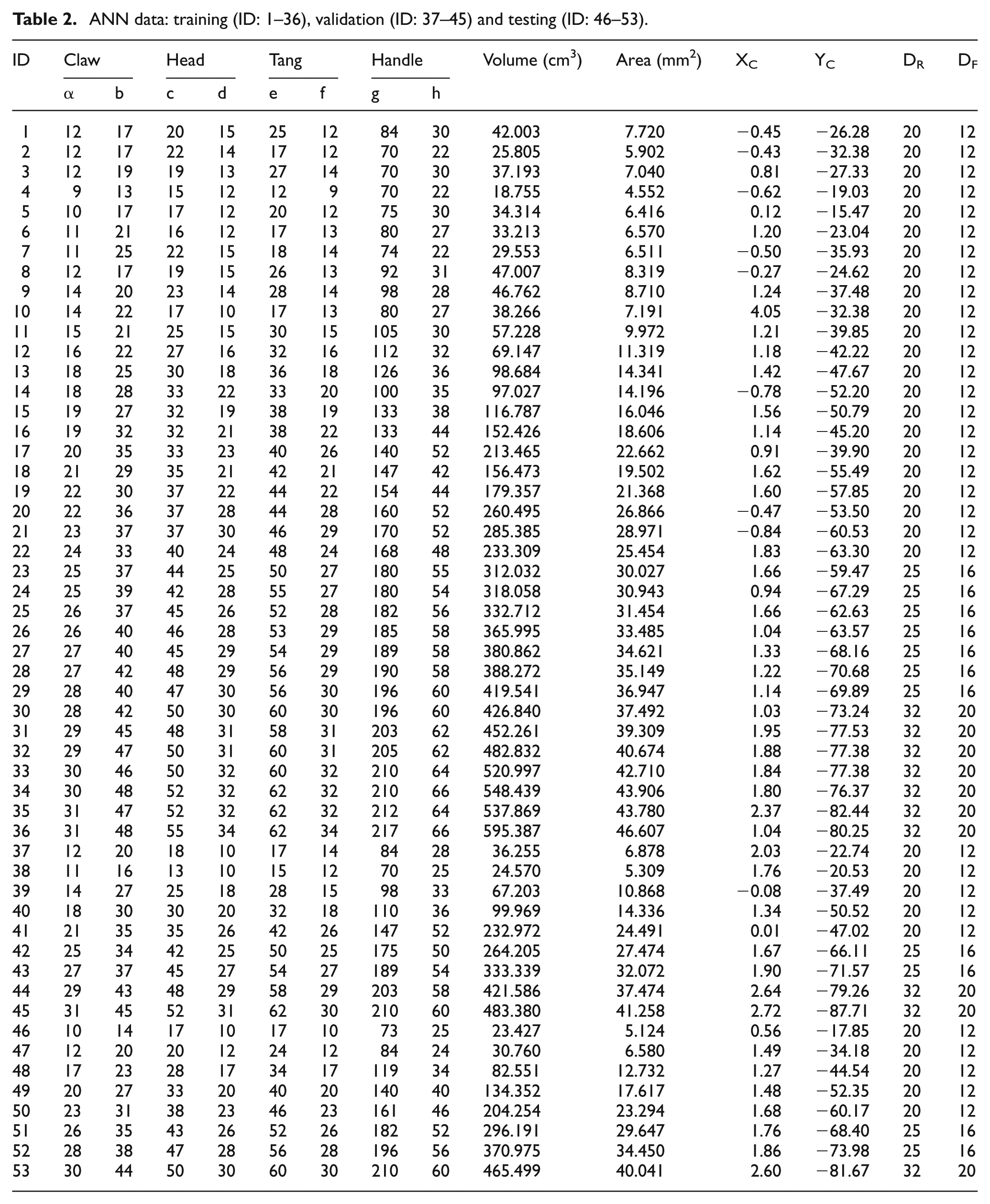
With regard to the hammer example, 53 variations were created by altering the eight control parameters corresponding to all four features. Table 2 presents the pertinent input data (eight element input vectors) and calculated output data (six element output vectors).

Table 2.

ANN data: training (ID: 1–36), validation (ID: 37–45) and testing (ID: 46–53).

ID	Claw		Head		Tang		Handle		Volume (cm³)	Area (mm²)	X_C	Y_C	D_R	D_F
	α	b	c	d	e	f	g	h
1	12	17	20	15	25	12	84	30	42.003	7.720	−0.45	−26.28	20	12
2	12	17	22	14	17	12	70	22	25.805	5.902	−0.43	−32.38	20	12
3	12	19	19	13	27	14	70	30	37.193	7.040	0.81	−27.33	20	12
4	9	13	15	12	12	9	70	22	18.755	4.552	−0.62	−19.03	20	12
5	10	17	17	12	20	12	75	30	34.314	6.416	0.12	−15.47	20	12
6	11	21	16	12	17	13	80	27	33.213	6.570	1.20	−23.04	20	12
7	11	25	22	15	18	14	74	22	29.553	6.511	−0.50	−35.93	20	12
8	12	17	19	15	26	13	92	31	47.007	8.319	−0.27	−24.62	20	12
9	14	20	23	14	28	14	98	28	46.762	8.710	1.24	−37.48	20	12
10	14	22	17	10	17	13	80	27	38.266	7.191	4.05	−32.38	20	12
11	15	21	25	15	30	15	105	30	57.228	9.972	1.21	−39.85	20	12
12	16	22	27	16	32	16	112	32	69.147	11.319	1.18	−42.22	20	12
13	18	25	30	18	36	18	126	36	98.684	14.341	1.42	−47.67	20	12
14	18	28	33	22	33	20	100	35	97.027	14.196	−0.78	−52.20	20	12
15	19	27	32	19	38	19	133	38	116.787	16.046	1.56	−50.79	20	12
16	19	32	32	21	38	22	133	44	152.426	18.606	1.14	−45.20	20	12
17	20	35	33	23	40	26	140	52	213.465	22.662	0.91	−39.90	20	12
18	21	29	35	21	42	21	147	42	156.473	19.502	1.62	−55.49	20	12
19	22	30	37	22	44	22	154	44	179.357	21.368	1.60	−57.85	20	12
20	22	36	37	28	44	28	160	52	260.495	26.866	−0.47	−53.50	20	12
21	23	37	37	30	46	29	170	52	285.385	28.971	−0.84	−60.53	20	12
22	24	33	40	24	48	24	168	48	233.309	25.454	1.83	−63.30	20	12
23	25	37	44	25	50	27	180	55	312.032	30.027	1.66	−59.47	25	16
24	25	39	42	28	55	27	180	54	318.058	30.943	0.94	−67.29	25	16
25	26	37	45	26	52	28	182	56	332.712	31.454	1.66	−62.63	25	16
26	26	40	46	28	53	29	185	58	365.995	33.485	1.04	−63.57	25	16
27	27	40	45	29	54	29	189	58	380.862	34.621	1.33	−68.16	25	16
28	27	42	48	29	56	29	190	58	388.272	35.149	1.22	−70.68	25	16
29	28	40	47	30	56	30	196	60	419.541	36.947	1.14	−69.89	25	16
30	28	42	50	30	60	30	196	60	426.840	37.492	1.03	−73.24	32	20
31	29	45	48	31	58	31	203	62	452.261	39.309	1.95	−77.53	32	20
32	29	47	50	31	60	31	205	62	482.832	40.674	1.88	−77.38	32	20
33	30	46	50	32	60	32	210	64	520.997	42.710	1.84	−77.38	32	20
34	30	48	52	32	62	32	210	66	548.439	43.906	1.80	−76.37	32	20
35	31	47	52	32	62	32	212	64	537.869	43.780	2.37	−82.44	32	20
36	31	48	55	34	62	34	217	66	595.387	46.607	1.04	−80.25	32	20
37	12	20	18	10	17	14	84	28	36.255	6.878	2.03	−22.74	20	12
38	11	16	13	10	15	12	70	25	24.570	5.309	1.76	−20.53	20	12
39	14	27	25	18	28	15	98	33	67.203	10.868	−0.08	−37.49	20	12
40	18	30	30	20	32	18	110	36	99.969	14.336	1.34	−50.52	20	12
41	21	35	35	26	42	26	147	52	232.972	24.491	0.01	−47.02	20	12
42	25	34	42	25	50	25	175	50	264.205	27.474	1.67	−66.11	25	16
43	27	37	45	27	54	27	189	54	333.339	32.072	1.90	−71.57	25	16
44	29	43	48	29	58	29	203	58	421.586	37.474	2.64	−79.26	32	20
45	31	45	52	31	62	30	210	60	483.380	41.258	2.72	−87.71	32	20
46	10	14	17	10	17	10	73	25	23.427	5.124	0.56	−17.85	20	12
47	12	20	20	12	24	12	84	24	30.760	6.580	1.49	−34.18	20	12
48	17	23	28	17	34	17	119	34	82.551	12.732	1.27	−44.54	20	12
49	20	27	33	20	40	20	140	40	134.352	17.617	1.48	−52.35	20	12
50	23	31	38	23	46	23	161	46	204.254	23.294	1.68	−60.17	20	12
51	26	35	43	26	52	26	182	52	296.191	29.647	1.76	−68.40	25	16
52	28	38	47	28	56	28	196	56	370.975	34.450	1.86	−73.98	25	16
53	30	44	50	30	60	30	210	60	465.499	40.041	2.60	−81.67	32	20

ANN model training

ANN training is performed on dedicated environments such as MATLAB. Optimum ANN architecture was determined by proprietary custom software that has been developed for that purpose and is extensively presented elsewhere.²⁹ Six individual ANNs were developed which predict two shape properties of the part (or die), namely, volume (or volume to be removed from the die) and area of the surface of the part (or die); two functional characteristics, namely, the axial distance of the centre of mass from the axis of the handle and the distance of the centre of mass of the part from the centre of the handle; and two manufacturing-related characteristics, namely, cutting tool diameter for roughing and finishing. Each ANN had eight inputs, namely, the two control parameters for each of the four features of the part. In order to achieve better training output, data were scaled so as their value ranges became similar. In particular, original volume and area values were divided by 1000.

The 53 vectors of the database were divided into three subsets for training, validation and testing consisting of 36, 9 and 8 vectors, respectively. This division into subsets was kept the same for all six ANN models. According to the Levenberg–Marquardt algorithm with early stopping that was employed, a training subset was used for pure training purposes, a validation subset was used to avoid overfitting through early stopping and a testing subset was used to check generalisation ability of the network.²⁸

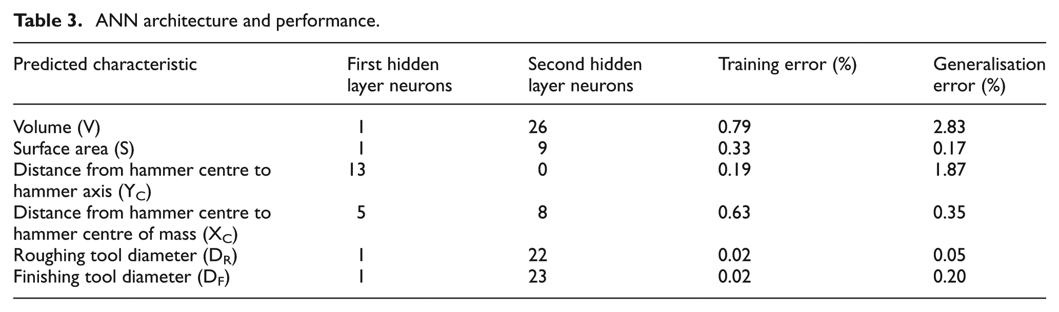
ANN response in respect of training is measured by the mean of the absolute value of the relative error for each training vector. The same holds for generalisation response. They may both be expressed on a 0–1 or % (0–100) scale. Table 3 presents architecture of the six ANNs developed and the respective responses. ANN performance in detail (i.e. for each individual vector used for training or testing) is indicatively presented in Figure 8 concerning two of the ANNs.

Table 3.

ANN architecture and performance.

Predicted characteristic	First hidden layer neurons	Second hidden layer neurons	Training error (%)	Generalisation error (%)
Volume (V)	1	26	0.79	2.83
Surface area (S)	1	9	0.33	0.17
Distance from hammer centre to hammer axis (Y_C)	13	0	0.19	1.87
Distance from hammer centre to hammer centre of mass (X_C)	5	8	0.63	0.35
Roughing tool diameter (D_R)	1	22	0.02	0.05
Finishing tool diameter (D_F)	1	23	0.02	0.20

Figure 8.

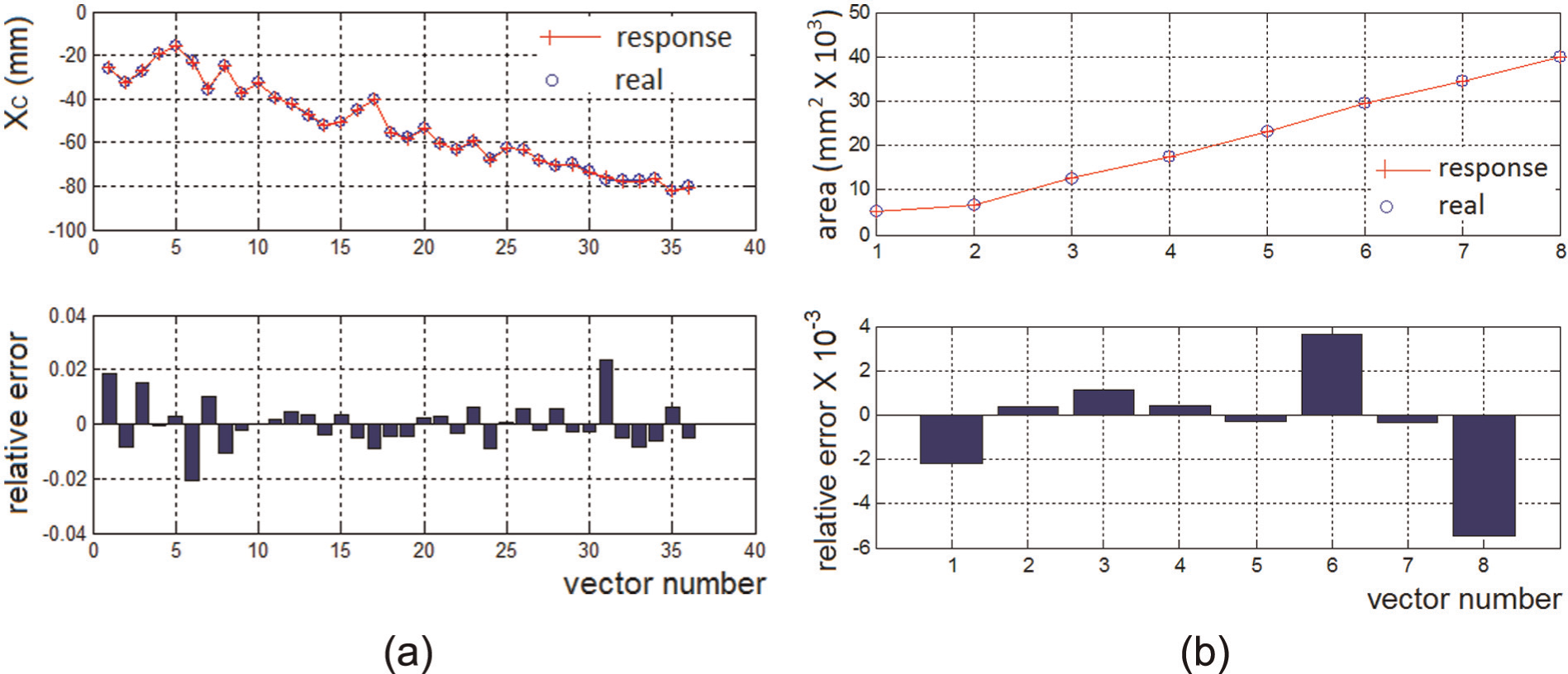
Indicative ANN performance: (a) training for distance X_C and (b) generalisation for area (S).

All ANNs exhibit excellent performance in terms of both training and, most importantly, generalisation with no sign of any tendency to memorise (overfit) data. Hence, ANNs can safely replace the CAD model in predicting volume and surface area of the designed part/die, as well as in calculating the two functional distances regarding the part’s centre of mass. In addition, ANNs can be substituted for the fuzzy system selecting cutting tool diameters.

Each ANN can be used in the optimisation part as a function embedded into the cost function used for assessing the design, thereby avoiding technical difficulties in linking dissimilar software to the optimiser through Application Programming Interfaces. Most importantly, ANNs function as surrogate models reducing execution time by orders of magnitude compared to parent models (CAD, CAM, etc.). This renders iterative optimisation algorithms practical given that they need to call the evaluator repeatedly, as discussed in the next section.

Design optimiser

The aim of the optimiser is to determine the best combination of feature control parameter values as assessed by a suitably defined evaluation function. The latter may combine several criteria, which, in addition, may need to be weighted by the designer. Different weighting schemes should be possible to explore by the designer.

In the general case, there will be a number of equivalent best combinations of control parameter values, which allows the designer the freedom of selection. When the number of parameters is large, the search space becomes too large to explore with conventional means. In this case, stochastic search via evolutionary algorithms such as the – classic by now – GAs seems imperative.

GAs

The main idea behind GAs is that subsets of the search space that contain good solutions can be identified by stochastic sampling which occurs iteratively and keeps a population of solutions which is gradually improved. The best members of this population after the latter has been allowed to mature constitute the (sub)optimal solutions. There are three main ingredients to a GA. First, each solution is coded as a string of values of the control parameters of the problem. This string is the chromosome and each element of the string is a ‘gene’. Usually, binary encoding is applied for each variable, but real encoding is possible, too. A predefined number of chromosomes constitute the population which evolves by keeping a certain number of good members (elitism) and replacing the rest by new ones as a result of genetic operators. Second, an evaluation function should be defined to allow assessment of any chromosome. Optimisation corresponds in minimising (or maximising) the value of this function. Third, a set of genetic operators similar to those found in biology should be defined to allow the population to evolve, thereby guiding the stochastic search.³⁰ The standard operators are selection, crossover and mutation (see Figure 9(a)). Selection identifies chromosomes of the population for reproduction. Crossover implements reproduction in terms of mutual exchange of genes between two selected chromosomes. Mutation adds variety to the population by changing the value of one or more genes of a chromosome with a generally low probability.

Figure 9.

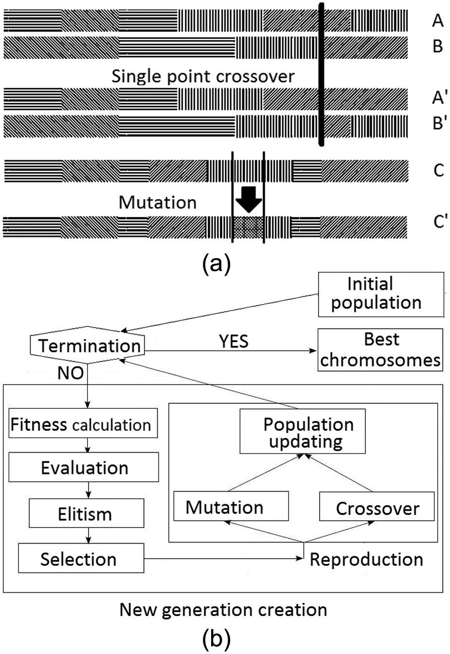
(a) Crossover and mutation and (b) GA overall functioning.

Genetic optimisation proceeds as shown in Figure 9(b). Note that fitness calculation for a chromosome should be skipped when constraints on the value of a parameter are violated, in which case an artificially extreme value is assigned to the fitness function as a kind of penalty. The loop reflecting evolution of the population is terminated according to various criteria, for example, after a predefined number of iterations (generations) or after a certain improvement in evaluation function value.

GA implementation

The GA for the hammer (die) design case was implemented in MATLAB as detailed next.

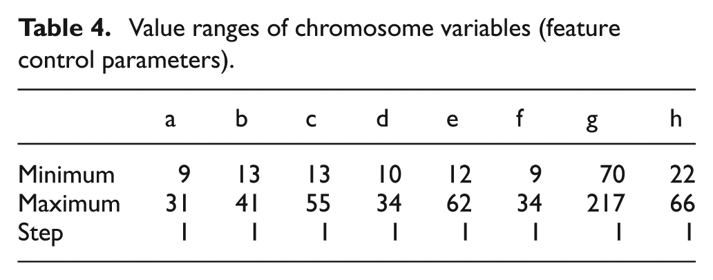
The chromosome consists of the eight feature control parameters defining the part. Their values are integer and encoding is binary. In this way, the length of the chromosome can vary depending on the value range of the parameters following the designer’s intent (see section ‘Parametric design of freeform surface parts’). The latter are shown in Table 4.

Table 4.

Value ranges of chromosome variables (feature control parameters).

	a	b	c	d	e	f	g	h
Minimum	9	13	13	10	12	9	70	22
Maximum	31	41	55	34	62	34	217	66
Step	1	1	1	1	1	1	1	1

The following function was defined for assessing design solutions

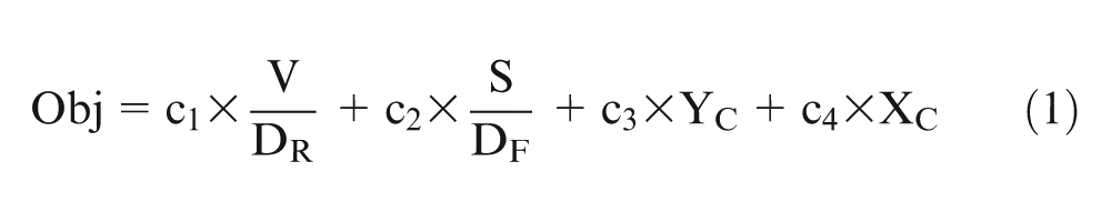
Obj = c_{1} \times \frac{V}{D_{R}} + c_{2} \times \frac{S}{D_{F}} + c_{3} \times Y_{C} + c_{4} \times X_{C}

(1)

where V stands for part volume; S for part surface area; D_R and D_F for roughing and finishing tool diameters, respectively; and Y_C and X_C for functional distances as depicted in Figure 5. All pertinent quantities are derived from the respective ANN metamodels (see section ‘ANN model training’). Minimisation of this function is sought.

The function consists of four parts or criteria. Note that roughing and finishing tool diameters have been determined from the decision support system as outlined in section ‘ANNs’ respecting the user’s intended relative significance of machining time and surface quality. This is taken to mean that minimum level of surface quality is safeguarded and any alternative solutions may be compared on the basis of machining time. Therefore, the first two parts of the objective function are interpreted as an indication of machining time. V/D_R favours low material volume to be removed faster the greater the tool diameter. Similarly, S/D_S favours low surface area of the part which will be scanned faster by larger tools. The last two parts of the function favour ‘balanced’ hammers, that is, (1) those with minimum distance between their centre of mass and the axis of the handle and (2) minimum distance between the centre of mass of the hammer and that of the handle.

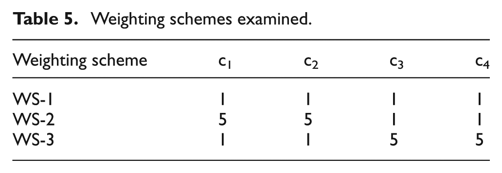
Constants c₁–c₄ define the relative weighting of the four parts (weighting scheme). In the course of experimentation, three different cases (weighting schemes) were examined (see Table 5).

Table 5.

Weighting schemes examined.

Weighting scheme	c₁	c₂	c₃	c₄
WS-1	1	1	1	1
WS-2	5	5	1	1
WS-3	1	1	5	5

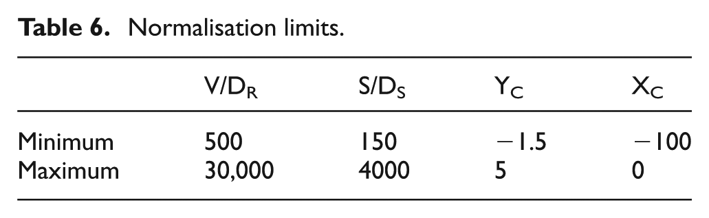
Comparison between evaluation function parts and their use in general require mapping of their value range to the interval [0,1], that is, normalisation (see Table 6).

Table 6.

Normalisation limits.

	V/D_R	S/D_S	Y_C	X_C
Minimum	500	150	−1.5	−100
Maximum	30,000	4000	5	0

Population size was set to 50, maximum number of generations to 100 and elitism to 4%, that is, 48 new chromosomes were produced in each generation. Stochastic universal sampling (SUS) was set as selection operator. Single point crossover (see Figure 9(a)) with a 70% probability for each chromosome pair was applied. Single gene mutation with 5% probability was set applying to binary genes (see Figure 9(a)). These values were arrived at after some experimentation to determine the corresponding sensitivity of the results.

Results and discussion

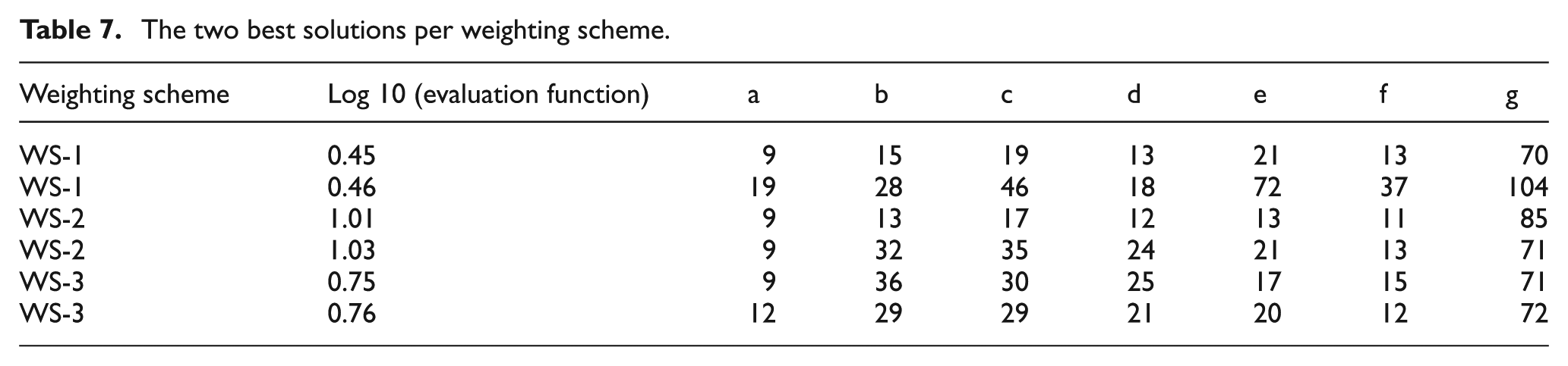
The GA was run 10 times for each weighting scheme. The best and the second best solutions in these runs were retained and are presented in Table 7. The results for the best solution in each weighting scheme are presented in Table 8.

Table 7.

The two best solutions per weighting scheme.

Weighting scheme	Log 10 (evaluation function)	a	b	c	d	e	f	g
WS-1	0.45	9	15	19	13	21	13	70
WS-1	0.46	19	28	46	18	72	37	104
WS-2	1.01	9	13	17	12	13	11	85
WS-2	1.03	9	32	35	24	21	13	71
WS-3	0.75	9	36	30	25	17	15	71
WS-3	0.76	12	29	29	21	20	12	72

Table 8.

Optimised properties results.

Optimisation properties	Weighting scheme
	WS-1	WS-2	WS-3
V (mm³)	20.585	44.238	43.739
S (mm²)	5.132	8.310	8.142
Y_C (mm)	−0.72	−2.28	−1.69
X_C (mm)	−23.50	−16.51	−44.47
D_R (mm)	20.00	11.24	19.88
D_F (mm)	11.98	6.93	12.92

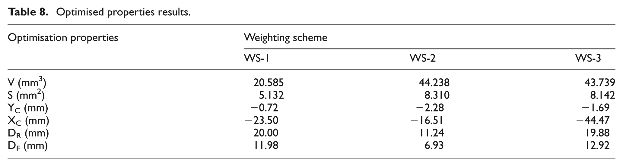
Figure 10 presents the evolution of the best solution for the three weighting schemes that were tried. They are obviously not comparable since each part of the evaluation function is weighted differently. In all cases, the solution was reached in less than 18 s on a personal computer (PC) with Core 2 Duo 2.4 GHz processor and 8 GB of RAM.

Figure 10.

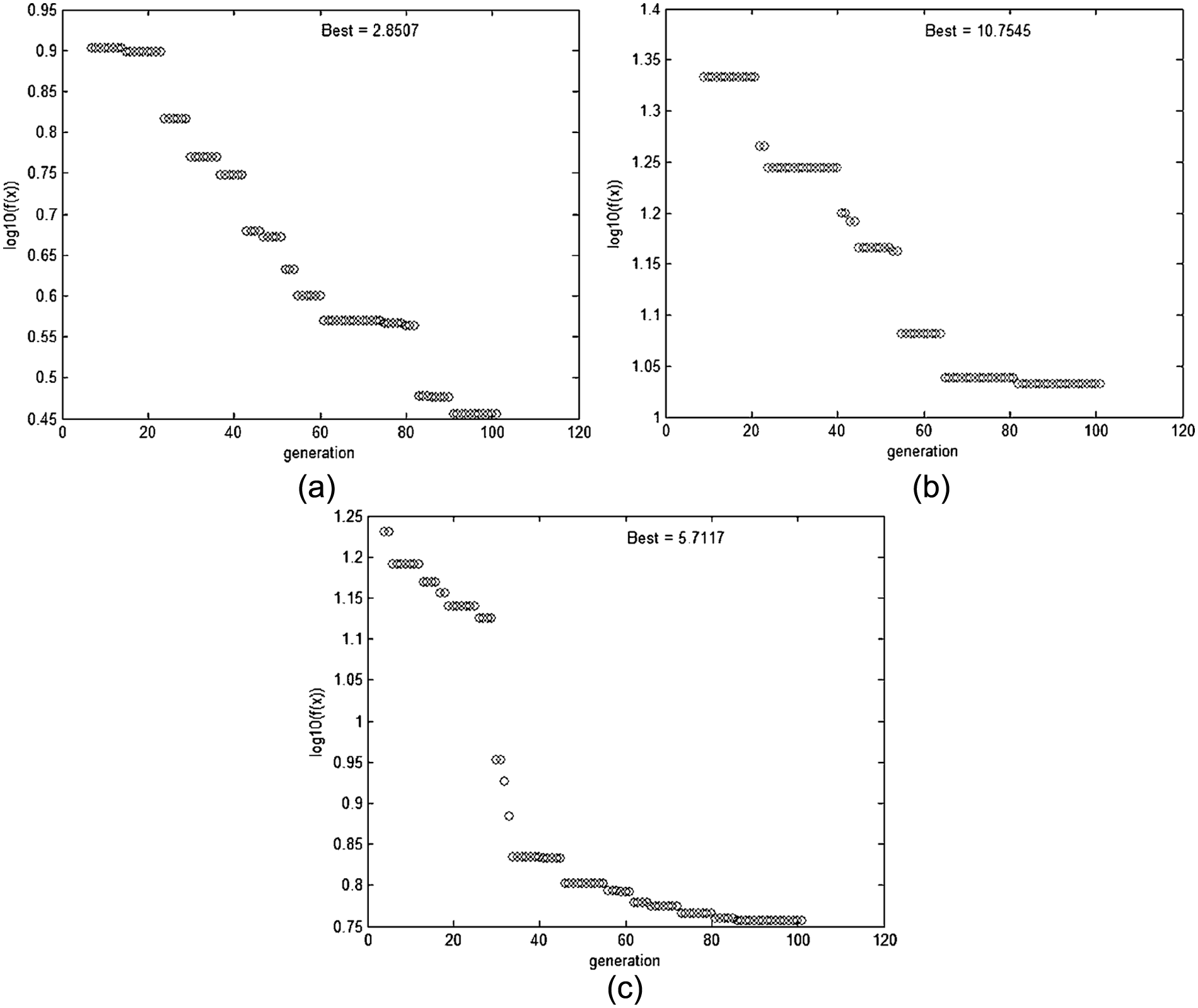
Evolution of the GA for the best solution: (a) WS-1, (b) WS-2 and (c) WS-3.

It becomes obvious from the above results that the influence of each control parameter of the features that comprise the designed part on the functional and manufacturing criteria set by the designer is not clear at all. This is even more conspicuous when the relevant constraints on these parameters are to be considered and, to go one step further, the constraints on the criteria as such, that is, in the terms of the evaluation function. Therefore, it was expected that many solutions selected by the GA for evaluation would be penalised and would be written off. Thus, a relatively large evolution population was chosen.

It is certain that more than one equivalent sub-optimal solution may exist. In the simplest of examples, the volume of the hammer may be the same for a hammer that has a large claw and a short handle or a small claw and a long handle. An evaluation function that combines functional and manufacturing criteria is expected to exhibit many local extrema.

An interesting observation concerns the variance of the evaluation function values for the n best chromosomes of the population. It is expected that some weighting schemes may result in smaller variance than others despite the fact that all individual criteria terms are normalised in the interval [0,1]. In the three schemes examined, the first and third seem to lead to smaller variance, but to say that with certainty, a large number of GA runs and statistical hypothesis testing would have been required.

It has to be noted that the evaluation function used in the examples presented was indicative. The evaluation function as such could be formulated with entirely different terms or with the same terms combined differently. For instance, it could have contained the inverse or the reverse of the roughing tool diameter, the finishing tool diameter, the inverse or reverse of the volume times distance X_C, the product of volume by distance Y_C and so on. In essence, each formulation of the evaluation function expresses pertinent design criteria, which may be widely different.

In practice, it is crucial for the designer to define an evaluation function that accurately represents his or her assessment of good and bad solutions as well as design parameter space acceptable and design constraints. For instance, material constraints and maximum stress or safety factor criteria may need to be considered, too, in the evaluation function. Of course, one might argue that, given the designer’s freedom in selecting criteria and constraints, there is a high chance that the same problem will yield totally different answers. The pertinent quasi-philosophical question as to which one of the various solutions is better is misleading since it is a matter of problem modelling and engineering feeling, merely meaning that the human is still in charge.

The GA optimiser is a proven fast means to explore a very large solution space. It was made more so in this work because its evaluation function works with surrogate (ANN) models. The latter are fast by definition since, in most cases in the DfX domain, they are expected to consist of just a few tens of neurons. Even in the case of information technology (IT) tools that are by definition fast, such as the fuzzy system employed in this work to select milling cutter diameter for die machining, it makes sense to use a surrogate model, so as to assess all variables involved in the evaluation function in a homogeneous way.

In the examples presented, ANN accuracy was high, which was achieved by using special custom-built software that optimises ANN architecture. This or analogous software is deemed indispensable in avoiding trial-and-error or brute-force enumerative approaches in configuring the ANNs.

The main merit of the approach is that ANNs, as surrogate models, provide a unifying method for modelling all criteria and constraints in product life-cycle phases, if there are enough examples to train them, and the GAs as optimisers may combine any ANNs in their evaluation function and explore the pertinent solution space fast.

Instead of ANNs, other interpolation or statistics-based approaches may be used. However, it is a well-documented fact that ANNs are superior to these approaches when it comes to not just representation of the particular data space but also generalisation, that is, response prediction, which is important in cases of strong non-linearities in the problem domain. Additional ANN advantages relating to robustness, upgradability and relatively low requirements in training data size are also well documented in standard literature.²⁸

Conclusion

The approach presented might be interpreted as an optimised Design-for-X system. A case study was used to demonstrate the capabilities of features as a shape parameterisation instrument, the ease of embedding them into stochastic-evolutionary optimisation of shape and the flexibility of employing various optimisation criteria through surrogate models, which are trained on the basis of engineering design/analysis tools.

Freeform surface features were a prerequisite enabling creation of variations within the framework of a part family and they need to be specific enough. Features are ultimately volumetric, but they are initially defined as wireframes using characteristic real or auxiliary curves/lines connected using design constraints. This is one novelty of the approach advocated.

The use of ANN surrogate models circumvents not only potentially lengthy solution assessment by the respective engineering tools but also problems of interfacing the optimiser to these tools, which are often not too trivial. Reliability of optimisation results depends on the accuracy of ANN models, that is, on their training quality in conjunction with the optimisation problem’s sensitivity regarding the pertinent variables, and this quality has to be ensured by a suitable approach and/or IT tool as demonstrated in this work.

In most practical cases, the distribution of extrema in the notional response hypersurface, let alone its type and shape, is not conspicuous, given the multitude of design criteria and constraints. It is expected that a multitude of combinations of design parameter values yield equivalent results. One repercussion of this is that it is hard to validate the optimisation result and another is the possible usefulness of Pareto techniques. The ultimate repercussion, however, is that the designer is left enough freedom to make the final choice out of a manageable number of alternatives.

Footnotes

Declaration of conflicting interests

The authors declare that there is no conflict of interest.

Funding

This work was funded by the PENED01 program (Measure 8.3 of the Operational Program Competitiveness, of which 75% is European Commission and 25% National Funding) under project number 01EΔ131.

References

ElMaraghy

. Knowledge management in collaborative engineering. Int J Collab Eng 2009; 1(1–2): 114–124.

Agte

Weck

Sobieszczanski-Sobieski

. MDO: assessment and direction for advancement – an opinion of one international group. Struct Multidiscip O 2009; 40(1–6): 17–33.

Brujic

Ristic

Mattone

. CAD based shape optimization for gas turbine component design. Struct Multidiscip O 2010; 41: 647–659.

Roy

Hinduja

Teti

. Recent advances in engineering design optimisation: challenges and future trends. CIRP Ann: Manuf Techn 2008; 57: 697–715.

Thiyagarajan

Grandhi

. Multi-level design process for 3-D preform shape optimization in metal forming. J Mater Process Tech 2005; 170(1–2): 421–429.

Bronsvoort

Bidarra

Nyirenda

. Developments in feature modelling. Comput Aided Design Appl 2006; 3(5): 655–664.

Vosniakos

G-C

. Investigation of feature-based product modelling for mechanical parts with free-form surfaces. Int J Adv Manuf Tech 1999; 15: 188–199.

Song

Vergeest

Bronsvoort

. Fitting and manipulating freeform shapes using templates. J Comput Inf Sci Eng 2005; 5(2): 86–95.

Pernot

Falcidieno

Giannini

. Modelling free-form surface using a feature-based approach. In: Proceedings of 8th ACM symposium on solid modelling and application, Seattle, WA, 16–20 June 2003, p.4. New York: ACM.

10.

Van den Berg

Bronsvoort

Vergeest

JSM

. Freeform feature modelling: concepts and prospects. Comput Ind 2002; 49(2): 217–233.

11.

Harzheim

Graf

. A review of optimization of cast parts using topology optimization, I – topology optimization without manufacturing constraints. Struct Multidiscip O 2005; 30: 491–497.

12.

Toussaint

Demoly

Lebaal

. PLM-based approach for design verification and validation using manufacturing process knowledge. J Syst Cybern Inform 2010; 8(1): 1–7.

13.

Edke

Chang

. Shape optimization of heavy load carrying components for structural performance and manufacturing cost. Struct Multidiscip O 2006; 31: 344–354.

14.

Korosec

Balic

Kopac

. Neural network based manufacturability evaluation of free form machining. Int J Mach Tool Manu 2005; 45(1): 13–20.

15.

Wang

H-J

Gao

C-H

. A computer aided tool selection system for 3D die/mould-cavity NC machining using both a heuristic and analytical approach. Int J Comp Integ M 2005; 18(8): 686–701.

16.

Castro

Antonio

CAC

Sousa

. Optimisation of shape and process parameters in metal forging using genetic algorithms. J Mater Process Tech 2004; 146(3): 356–364.

17.

Maropoulos

Ceglarek

. Design verification and validation in product lifecycle. CIRP Ann: Manuf Techn 2010; 59: 740–759.

18.

Molcho

Zipori

Schneor

. Computer aided manufacturability analysis: closing the knowledge gap between the designer and the manufacturer. CIRP Ann: Manuf Techn 2008; 57: 153–158.

19.

Gao

Liu

. Selection of green product design scheme based on multi-attribute decision-making method. Int J Sustain Eng 2010; 3(4): 277–291.

20.

Shi

Chen

Peng

. A new approach of die shape optimization for sheet metal forming processes. J Mater Process Tech 2004; 152(1): 35–42.

21.

Cappello

Mancuso

. A genetic algorithm for combined topology and shape optimisations. Computer Aided Design 2003; 35(8): 761–769.

22.

Liakopoulos

PIK

Kampolis

Giannakoglou

. Grid-enabled, hierarchical distributed metamodel-assisted evolutionary algorithms for aerodynamic shape optimization. Future Gener Comp Sy 2008; 24: 701–708.

23.

Park

Dang

. Structural optimization based on CAD–CAE integration and metamodeling techniques. Computer Aided Design 2010; 42(10): 889–902.

24.

Oudjene

Ben-Ayed

Delameziere

. Shape optimization of clinching tools using the response surface methodology with Moving Least-Square approximation. J Mater Process Tech 2009; 209(1): 289–296.

25.

Yao

Chen

Ouyang

. A surrogate based multistage-multilevel optimization procedure for multidisciplinary design optimization. Struct Multidiscip O 2012; 45: 559–574.

26.

Lewis

Murray

Mattson

. A design optimization strategy for creating devices that traverse the Pareto frontier over time. Struct Multidiscip O 2011; 43: 191–204.

27.

Giannakakis

Lipari

Vosniakos

G-C

. Fuzzy selection of milling tool diameters and strategies for dies with sculptured surfaces. J Mach Form Technol 2009; 1(1–2): 17–34.

28.

Gurney

. An introduction to neural networks. London: CRC Press, 1997.

29.

Benardos

Vosniakos

G-C

. Optimising feedforward artificial neural network architecture. Eng Appl Artif Intel 2007; 20(3): 365–382.

30.

Mitchell

. An introduction to genetic algorithms. Cambridge, MA: The MIT Press, 1998.

Multi-disciplinary design optimisation of mechanical parts with freeform surfaces: Case study encompassing manufacturing criteria

Abstract

Keywords

Introduction

Parametric design of freeform surface parts

Notions

Example

Discussion

Modelling and optimisation

Evaluation criteria

Functional criteria

Manufacturing criteria

Metamodel creation

ANNs

ANN training database creation

ANN model training

Design optimiser

GAs

GA implementation

Results and discussion

Conclusion

Footnotes

Declaration of conflicting interests

Funding

References