
Abstract
Mechanical products are usually made by assembling many parts. Among the different types of links, bolts are widely used to join the components of an assembly. In a bolting, a clearance exists among the bolt and the holes of the part to join. This clearance has to be modelled in order to define the possible movements agreed to the joined parts. To model a joint with clearance between two components is the aim of this work. This model takes part of a tolerance analysis model for rigid parts developed to overcome some limits of the literature’s works. It allows the assembly design to choose the tolerances on the basis of their impact on the assembling of the components and on the functional requirements. It adopts the simplified hypothesis that each surface maintains its nominal shape, that is, the effects of the form deviations are neglected. The proposed model has been successfully applied to a case study, a belt drive.
Introduction
Mechanical products are usually made by assembling different parts, and their quality is guaranteed by the respect of some functional requirements assigned on the whole assembly. Being the dimensional and the geometrical tolerances applied to the assembly components, in order to limit the deviations from the nominal due to the manufacturing process, the respect of the functional requirements depends on the cumulative effect of the tolerances applied to the single components and on the assembly constraints.
Tolerance analysis aims to study the accumulation of dimensional and/or geometric variations resulting from a stack of dimensions and tolerances. It is the fundamental tool to allocate the tolerances on the single components by solving the trade-off between the quality and the cost of the whole assembly. 1 Requicha2,3 was the first researcher to introduce the mathematical definition of the tolerance’s semantic. The first approach to tolerance analysis was the linear chains of dimensions. 4
Thereafter, many approaches to tolerance analysis have been developed by the literature. One approach is called vector loop; it represents the dimensions of an assembly by means of vectors.5–7 A vector may represent a component dimension or an assembly dimension. Chains or loops are built up with vectors in order to evaluate the effects of those dimensions on the interesting assembly dimensions. CE/TOL® is a software package that implements the vector loop model.
An alternative family of models is called variational model; it was developed by Martino and Gabriele, 8 Boyer and Stewart 9 and Gupta and Turner. 10 There are many software packages based on variational model, such as 3-DCS of Dimensional Control Systems® and VisVSA of UGS®. The variational model represents the variability due to tolerances and assembly constraints on an assembly through a parametric mathematical model. 11 It uses differential homogeneous transformation matrices to represent the dimensional and geometrical variations affecting a part. Whitney 4 has widely dealt with the variational model for both rigid and compliant parts by worst-case or statistical approaches.
A further approach of the literature is the matrix model. It gives an explicit mathematical representation of the boundary of the spatial region enveloping all displacements due to the variability sources. 12 To describe any roto-translational variation of a feature, a displacement matrix is adopted; it is a homogeneous transformation matrix.
There is an approach called Jacobian model too. It derives from the kinematic chains of robotics; the small deviations due to a tolerance are represented by six virtual joints that are the 6 degrees of freedom of a rigid part.13,14
Another approach, called Torsor model, uses screw parameters to represent three-dimensional (3D) tolerance zones. 15 Screw parameters are commonly used in kinematics to describe motion. The Torsor model uses the screw parameters to represent the region where a surface is allowed to move, that is, the tolerance range. To overcome the limits of both the approaches known as Jacobian and Torsor, in the last years, the unified Jacobian–Torsor model has been developed. It uses the Torsors to evaluate the displacements of the virtual joints due to the applied tolerances. It introduces the Jacobian matrix to put into relationship the functional requirements with the virtual joints.16,17
The tolerance map is the model developed at the Arizona State University.18,19 A Tolerance-Map (T-Map) is built by representing the displacements of a feature or of an assembly by a solid of points in n-dimensions. The stack-up equations are generated by overlaying the coordinates of the T-Map. The model proposed by the literature deals with joints with contact between the coupled parts.
Recently, the joints with clearance have been taken into account. There are different ways of modelling joints with clearance by inserting a clearance vector into the functional relationship. The first possibility is that the clearance vector is defined according to worst-case 20 and statistic scenarios. 21 The next step is to determine the clearance vector due to a certain joint force 22 Kuo and Tsai 23 have developed a model to evaluate the minimum gap in an assembly that affects its performances. The mathematical approaches developed by Davidson and Shah, 24 Giordano et al. 25 and Teissandier et al. 26 allow to calculate the composition of tolerances by Minkowsky sum of deviation and clearance domains, to calculate the intersection of domains for parallel kinematic chain and to verify the inclusion of a domain inside the other one. Qureshi et al. 27 used the same mathematical representation, but they added the compatibility domain that represents the composition relations of displacements in the various topological loops, and the mathematical formulation based on the quantifier notion. In Walter et al., 28 an integrated tolerance analysis approach for a crank mechanism inside combustion engine is presented taking into account link length deviations, clearance at the conrod big end bearing and elastic deformation of the crankshaft. In Mishra et al., 29 the effect of joint clearances on path generation of a mechanism is studied. However, many doubts remain on a general representation of joints with clearance inside a tolerance analysis model.
Therefore, the aim of this work is to present a general approach to model a joint with clearance between two components inside a variational model for tolerance analysis. The variational tolerance analysis model was developed for rigid parts to overcome some limits of the literature’s works. 30 The developed joint with clearance model allows the functional design of a mating, that is, the choice of the tolerances on the basis of their effect on the effective assembling of the components and on the functional requirements of the whole assembly. It adopts the simplified hypothesis that each surface maintains its nominal shape; that is, the effects of the form deviations are neglected. The proposed approach has been tested on a case study where the holes have dimensional and position tolerances.
In the following, the variational tolerance analysis model inside which it is inserted the modelling of the joints with clearance is deeply presented (section ‘Variational tolerance analysis model’). Therefore, the proposed model of a joint with clearance is deeply described (section ‘To model joints with clearance’), and then, it is applied to model a linkage between two parts by a planar contact surface and two bolts (section ‘Case study’). Finally, the model is applied to an industrial application, a belt drive (section ‘Industrial application example’).
Variational tolerance analysis model
Tolerance analysis aims to evaluate the cumulative effect due to the tolerances of the assembly components on the functional requirements of the whole assembly. 31 A functional requirement may be represented by an equation, whose variables are the model parameters. This equation is called stack-up function. The model’s parameters depend on the dimensions and the tolerances assigned to the assembly components. In this article, the assembly components are considered rigid. A stack-up function may be written as
where FR is the considered functional requirement, p1, …, pn are the model parameters and f(p) is the stack-up function, which is usually not linear.
A functional requirement is usually a dimension or a geometric relationship between two features. Its equation is obtained by means of the Euclidean geometry that is applied to the features or to the points of the features that define the functional requirement.
To define a stack-up function, a sequence of steps is needed that allow to model each component’s geometric variations due to the applied tolerances, the geometric variations between couple of components due to the assembling process and the functional requirements of the assembly. The first step creates a local model of tolerance analysis, the second a global model of tolerance analysis and the third creates the stack-up function of the global model (see Figure 1).
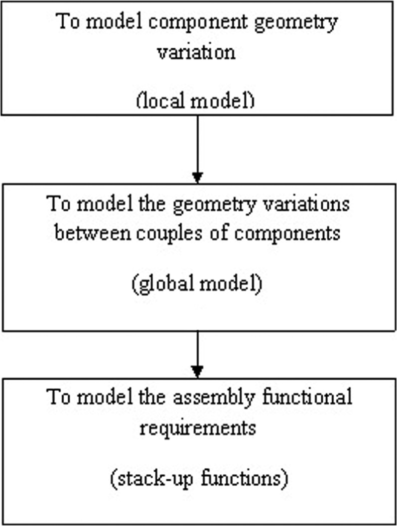
Frame of a tolerance analysis model.
The developing of the local model means to define the range of variation of the model’s parameters from the tolerances assigned to the component of the assembly. This means identifying, for each tolerance applied to each feature of each assembly component, the ranges of rotation and translation of the barycentre of the nominal feature due to the applied tolerance. Those rotations and translations are the model’s parameters, whose ranges are bounded by the ranges of the applied tolerance.
The developing of the global model means to define the range of variation of the model’s parameters from the variability of the coupled features during the assembly. The variability of the coupled features, by which the link among the parts is made, depends on the tolerances applied to the features themselves and by the assembly conditions.
Finally, to derive the stack-up functions it is needed that the global model has to be able to approach to the joints that give a linear structure of the FR equation (stack-up function) and to the joints that carry out to a complex structure of the FR equation (network function), as shown in Figure 2.
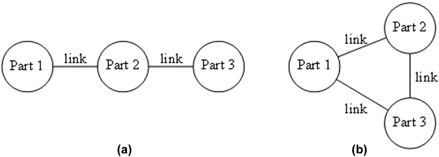
(a) Linear stack-up function and (b) network stack-up function.
Local model
Typically, each feature has its local datum reference frame (DRF), while each component and the whole assembly have their own global DRF. In the nominal condition, the homogeneous transformation matrix (called
where
If a feature may not be directly referred to the global DRF, it is reported to it through a chain of features. To calculate the total matrix, it is sufficient to make the product of the single contributions as shown in Figure 3, which is valid for the case of two transformations.
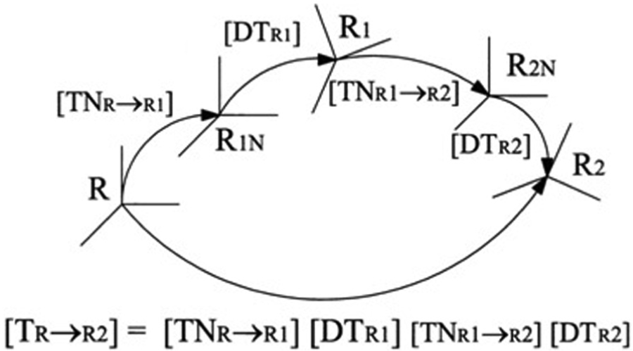
Model of a stack-up function in a part.
All the tolerance kinds, that is, dimensional, form, orientation and location, have to be represented by the local model. The local model has to deal with the Envelope Principle 32 or the Independence Principle. 33 The local model should be able to define the range of variation of model’s parameters, when more than one tolerance is applied to the same feature. All these aspects are solved by the developed model and all the details are discussed in Polini. 30
Global model
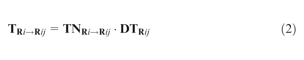
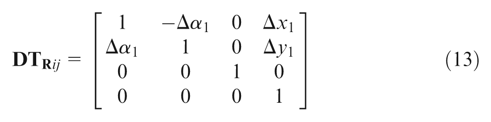
Typically, the relative location of the parts is expressed by means of parameters that constitute the differential homogeneous transformation matrix
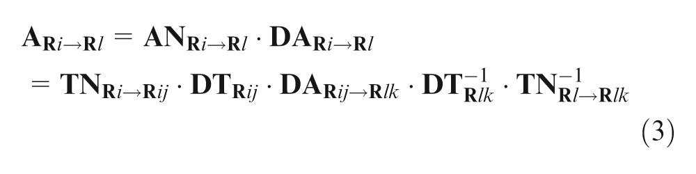
where
The differential assembly matrices
The global model should be able to schematize the joints with contact and the joints with clearance between the coupled features.
Stack-up functions
Once the assembly parameters are known, all features can be expressed in the same global DRF of the assembly
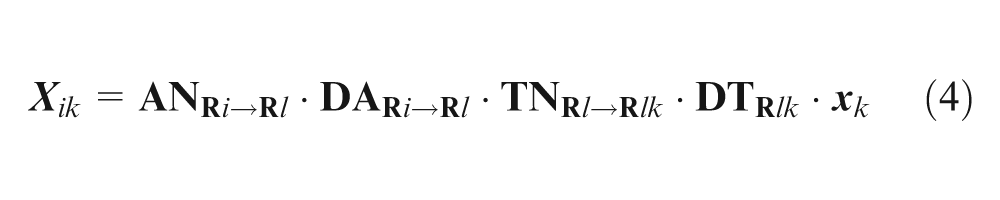
where
Then, the equations of the functional requirements are defined by applying the analytical geometry. The stack-up functions may be solved by means of a worst-case or a statistical approach.
34
The worst-case approach defines the worst configurations of the assembly (i.e. those configurations due to the build-up of the smallest and the largest values of the ranges of the tolerances applied to the components of the assembly) that respect the assigned tolerances. It involves an optimization (maximization and/or minimization) under constraints that are the assigned tolerances. There are many methods proposed by the literature to use a worst-case approach.
35
A statistical approach translates each tolerance applied to a component of an assembly into one or more parameters of the stack-up function. A probability density function (PDF) is assigned to each parameter. The PDF depends on both the manufacturing and the assembly processes. A Gaussian PDF is usually adopted since it is easy to handle. Moreover, it is very hard to estimate the PDF of a tolerance of a component by analysing the experimental data of the manufacturing process. An assumption commonly adopted is to consider independent the model’s parameters. The statistical approach calculates the PDF of the FR by means of Monte Carlo simulation36,37 and the range of variation of the FR as
To model joints with clearance
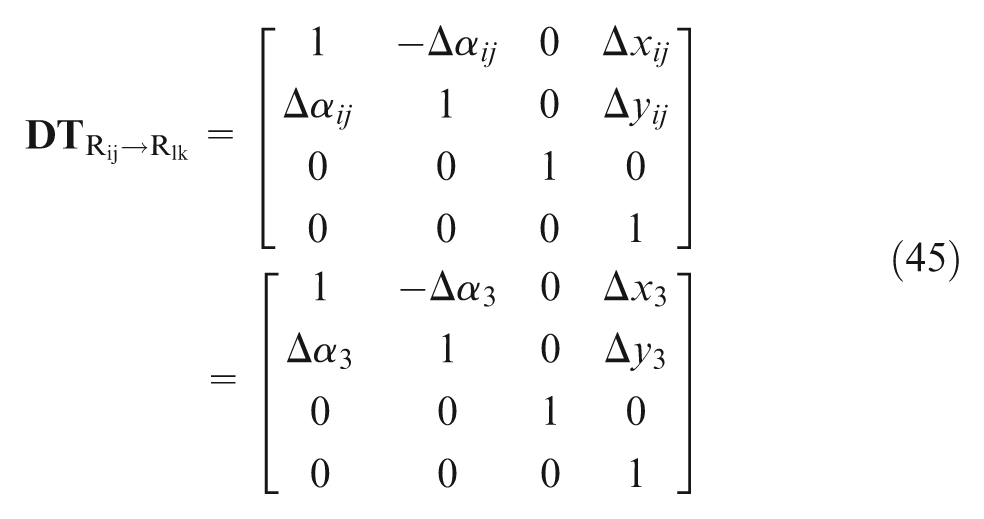
When two parts are assembled, the coupled surfaces constitute the joint. If the joint involves a clearance, the clearance affects only some of the six small kinematic adjustments that define the position of a part as regards the other. At least two surfaces are usually in contact; they lock 3 degrees of freedom: the translation along the axis perpendicular to the surfaces in the contact point (indicated as z) and the rotations around the transversal axes (x and y), as shown in Figure 4. The general structure of a clearance differential matrix is
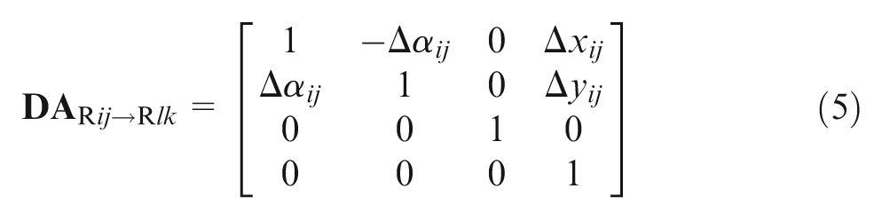
where Δxij and Δyij are the translations along the x- and y-axes of the surface k as regards the surface j evaluated in the DRF
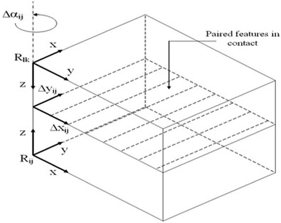
Scheme of a joint with clearance.
To evaluate the model parameters of a clearance differential matrix (Δxij, Δyij and Δαij), it is necessary to observe that they depend on the cumulative effects of the assembly conditions required among the coupled surfaces of the joint. The first constraint required on the surfaces of the joint is usually the one which imposes that the two surfaces have to remain in contact; it determines the structure of the clearance differential matrix, as shown in equation (5). To each of the other single constraints, the domains of the admissible values of the model parameters (Δxij, Δyij and Δαij) have to be considered; it is called single admissible domain (SAD). These SADs may be plotted on a 3D space, axes of which are the small kinematic adjustments (Δxij, Δyij and Δαij); this space is called admissible solution space (ASS). Therefore, the cumulative admissible domain (CAD) of all the constraints can be easily evaluated as the intersection domain of all the SADs (Figure 5). If the CAD is empty, the assembly is not possible. If the CAD contains only a point, the assembly is possible, and it is determined as the configuration expressed by the admissible point. If the CAD contains a set of points, the boundary that encloses them may be determined. Once the boundary of the domain of the cumulative effects of the joining conditions that are required among the coupled surfaces of the assembly is evaluated, the tolerance analysis model can be defined by imposing this boundary. It is an additional constraint acting on the model parameters in the worst-case approach. It is the range of the PDF that is assigned to the model parameters in the statistical-case approach.
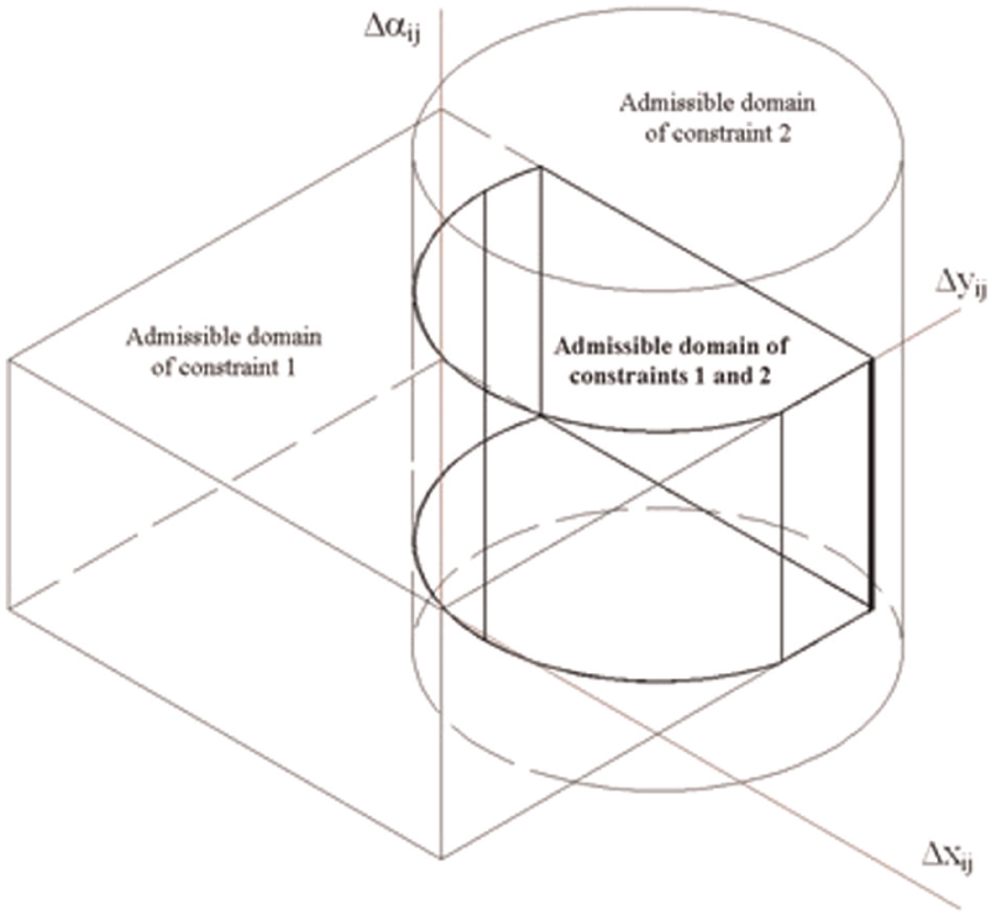
Single admissible domains of the constraints and cumulative admissible domain.
Case study
A mechanical linkage is the type of joint with clearance most widely used in industrial application. Despite their spread, a bolting is usually dimensioned only on the basis of the load that has to be transferred from a component to the other. The tolerances are usually assigned on the surfaces involved in the joint on the basis of the experience, while their influence on the effective assembling of the components or on the functional requirements of the whole assembly is rarely taken into account.
To show the effective application of the proposed general model, it has been developed for this specific case. In a bolting, two parts are mated by joining a planar contact surface and a pattern of bolts. This work considers a pattern of only two holes, but the proposed model may be easily extended to more than two holes. The two holes are considered independent and the applied tolerances are shown in Figure 6.
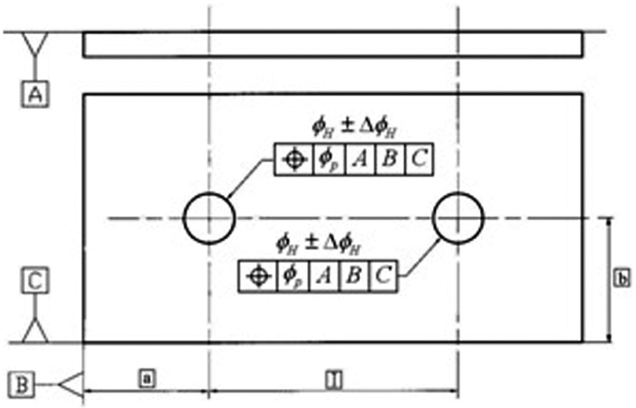
Tolerances applied to the components of the linkage.
The tolerances are applied according to the envelope rule (or Rule 1) of the ASME standard.
32
The relative position between the two parts deviates from the nominal since dimensional and location tolerances are applied to the holes of the plates and to the bolts. The local DRF of feature j of part i (
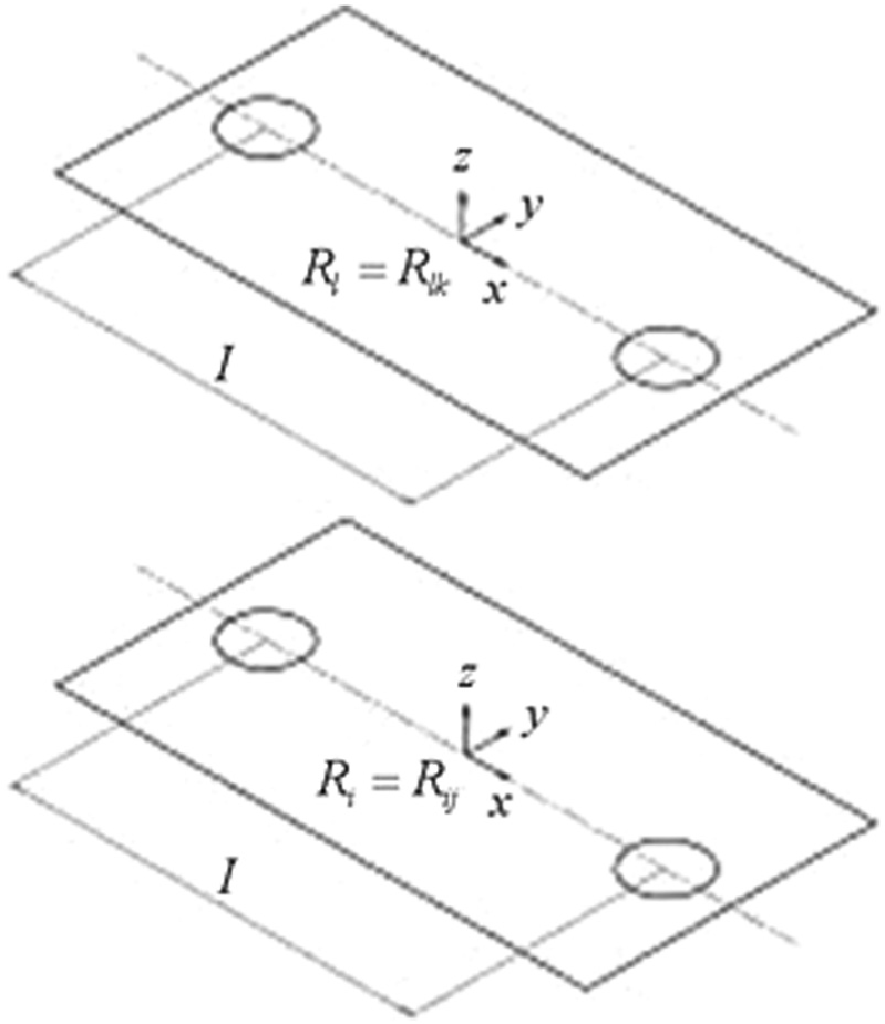
Position of the local DRFs for the linkage.
Once these assumptions are fixed
and then equation (3) becomes
Differential matrices
In the following, the first part is called part 1 and its parameters have 1 as the first subscript. The second part is called part 2 and its parameters have 2 as subscript. The holes on the left have subscript 1, and the holes on the right have subscript 2. For example, the hole on the right of the first part is called hole 12. To evaluate the differential transformation matrix
Deviation of part 1 of the linkage.
The
and the real distance between the axes is
where
If a worst-case approach is carried out, the auxiliary model parameters have to be constrained by the following relationships
If a statistical-case approach is carried out, the auxiliary model parameters are stochastic variables with a PDF. The modules


The angles
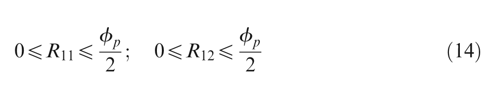
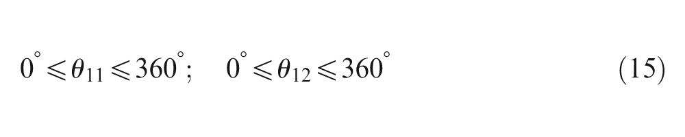
The differential transformation matrix
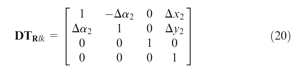
where

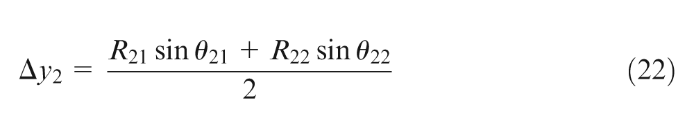
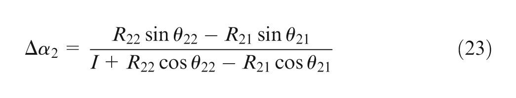
and the real distance between the axes is
where R22, R21, θ22 and θ21 are auxiliary parameters of the model that quantify the position deviation of the two holes.
If a worst-case approach is carried out, the auxiliary model parameters have to be constrained by the following relationships
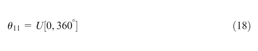
If a statistical approach is carried out, the auxiliary model parameters are stochastic variables with the following PDF

Bolts
The only tolerance considered for the two bolts is the dimensional one applied to their diameters. Once the bolt on the left is called bolt 1 and the bolt on the right is called bolt 2, the bolt diameter has to be constrained by the following relationships according to the worst-case approach
where
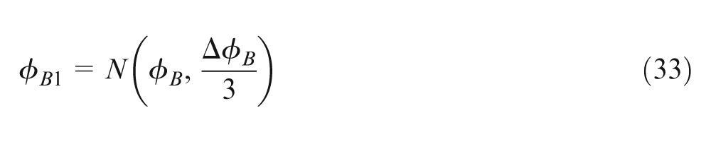
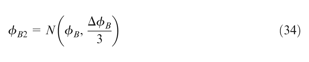
If a statistical approach is applied, the bolt diameters are stochastic variables following Gaussian PDF with mean value equal to the nominal (0) and SD equal to 1/6 of the dimensional tolerance applied to the diameter (three-sigma paradigm)
Clearance differential matrix
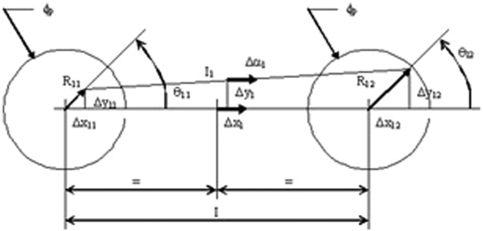
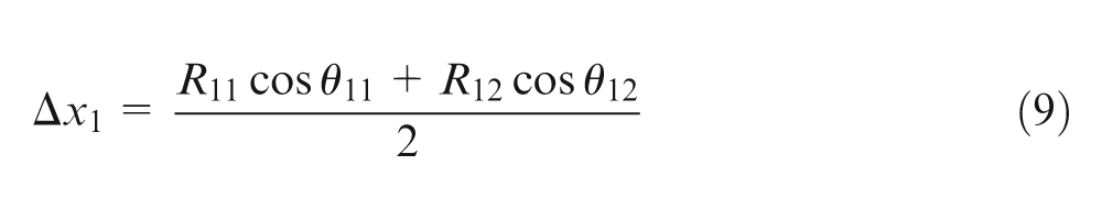
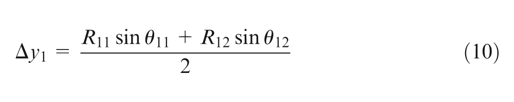
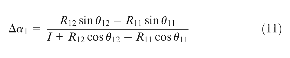
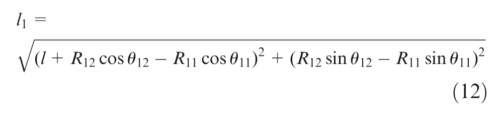
To evaluate the clearance differential matrix
where I1 and I2 are the real distances between the centres of the holes previously calculated.
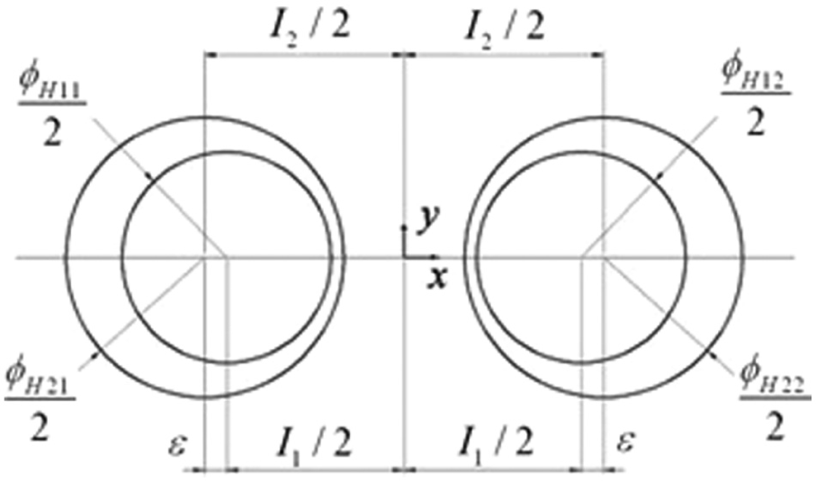
Deviations between the parts.
If the position of the centre of the two left holes is centred, the assembling condition is satisfied if
where
If the condition (36) is verified, the distance expressed by equation (37) is not negative.
Radial deviation on the left bolt.
In the same way, for the right bolt, it is
and
where
Therefore, it is possible to represent on the ASS the SAD of the two bolts, which are circles (see Figure 11).
SAD and CAD of the bolts of the linkage.
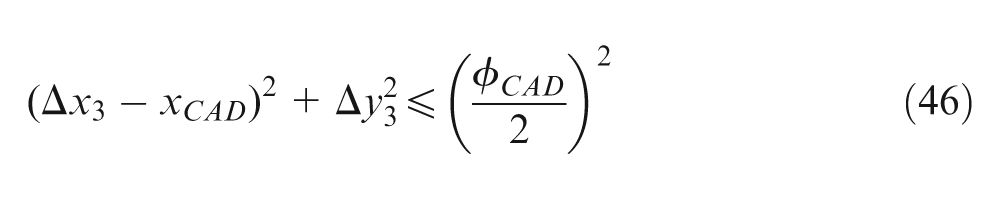
The CAD of the two bolts is the intersection of the two domains; it is shown as dashed lines in Figure 11. Considering that the deviations are usually small, this CAD may be approximated as a circle, as shown in Figure 12
where
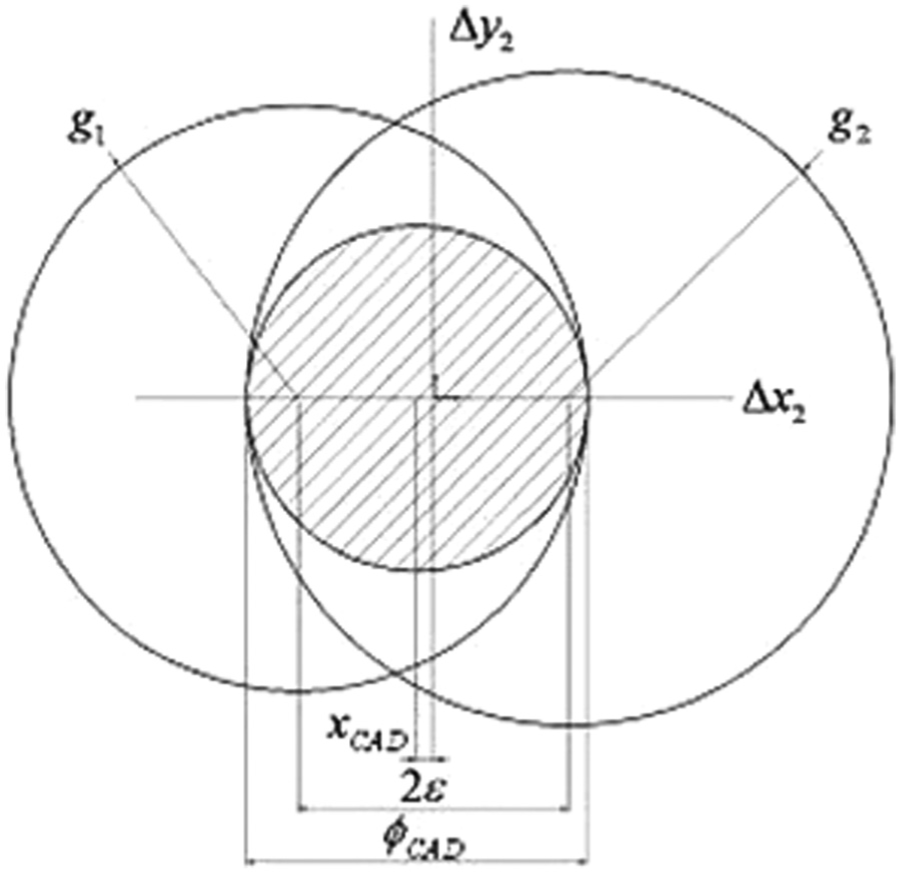
Approximated CAD of the bolts of the linkage.
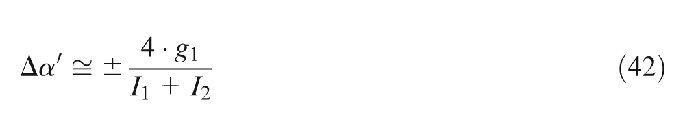
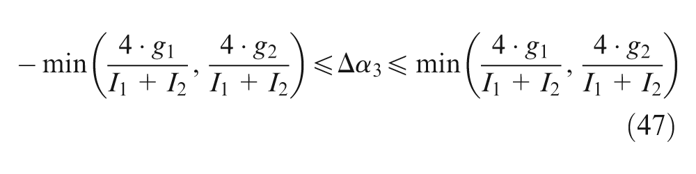
Finally, the rotation parameter
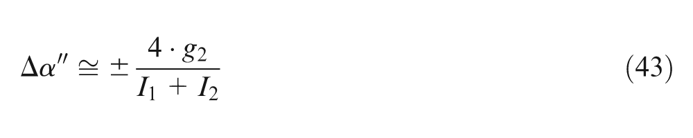
while for the right bolt
Therefore, it may be expressed as the smallest of equations (42) and (43)
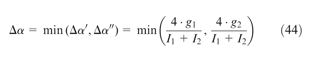
It is supposed that g1 and g2 are not negative, differently the assembly is not possible.
The clearance differential matrix may be expressed as
whose small kinematic adjustments in the worst-case approach have to be constrained by the following relationships
They are stochastic variables following a uniform PDF in the statistical approach

Finally, the assembly transformation matrices (3) and (8) are expressed by neglecting the terms of higher order
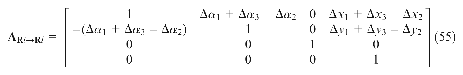
with the usual symbols.
Modifier material conditions
If the position tolerances are applied to the holes with a modifier material condition, for example, the maximum material condition (MMC), they will appear as shown in Figure 13.
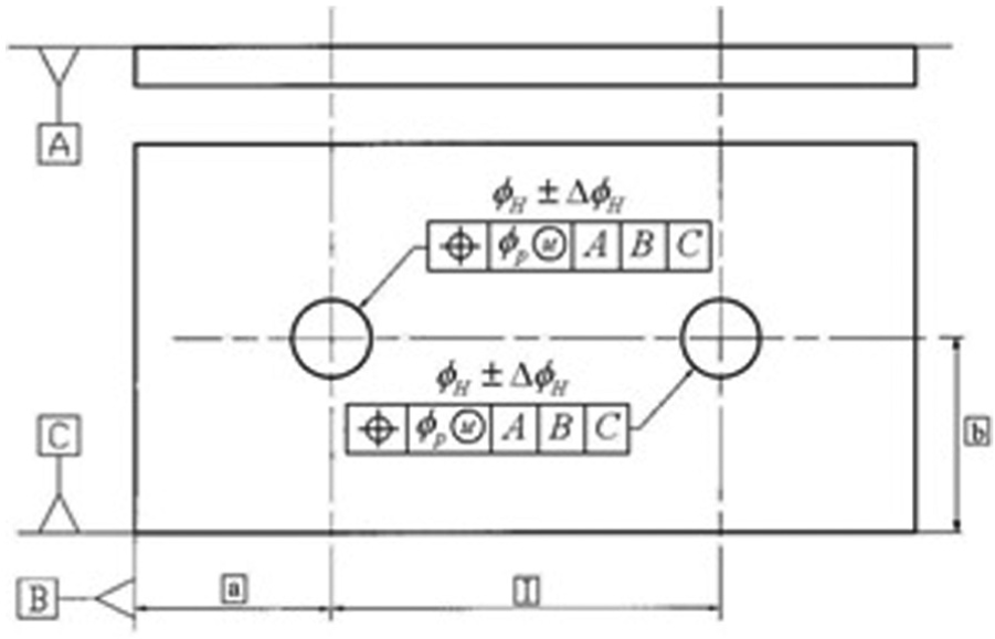
Application of MMC to the linkage.
The model previously shown remains valid, but it should take into account the bonus due to the positional tolerances of the holes. In fact, the value of the positional tolerance range of a hole is not constant, but it depends on the real diameter of the hole. Being the bonus given from the difference between the real value and the value at MMC
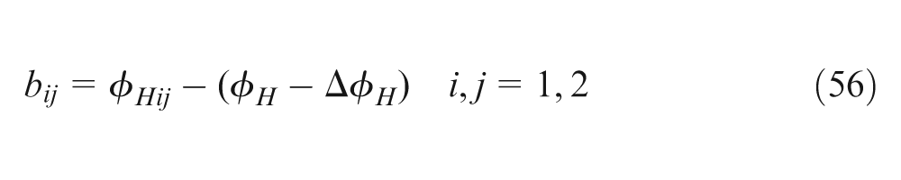
where bij is the bonus of the ijth hole,
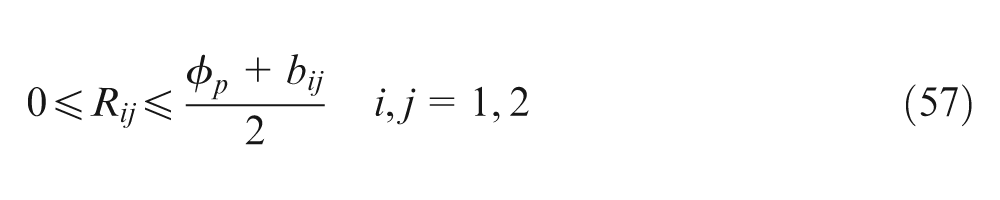
The bonus increases the admissible range of the positional tolerance; for the worst-case approach, it may be expressed as
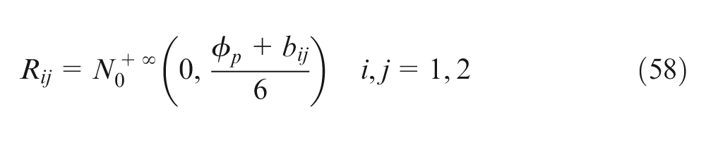
while for statistical-case approach as
Industrial application example
The drawing in Figure 14 shows an assembly constituted by five components: a top plate, a right and a left axle support, an axle and a wheel. Its structure looks like a simplified belt drive. Therefore, dimensional, position, orientation and form tolerances are assigned to each component by taking into consideration the assembly functional requirements. A possible design of the assembly parts is shown in Figure 15, that is, the starting basis of 3D tolerance analysis.
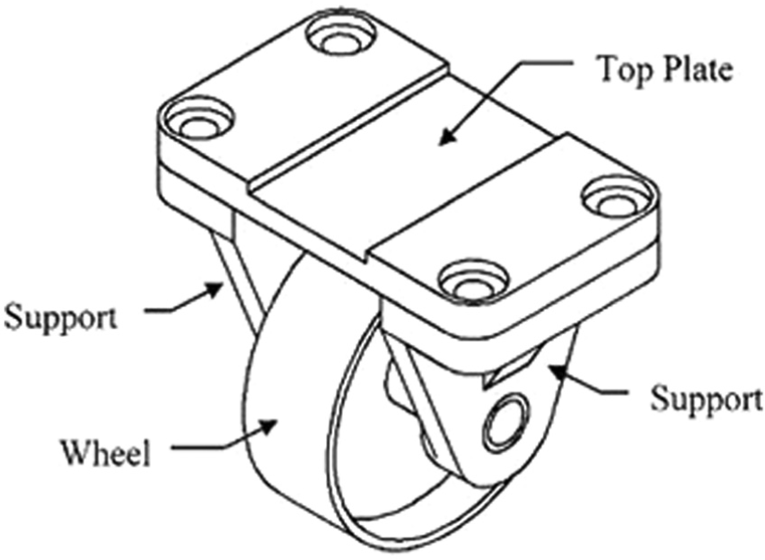
Industrial application example.
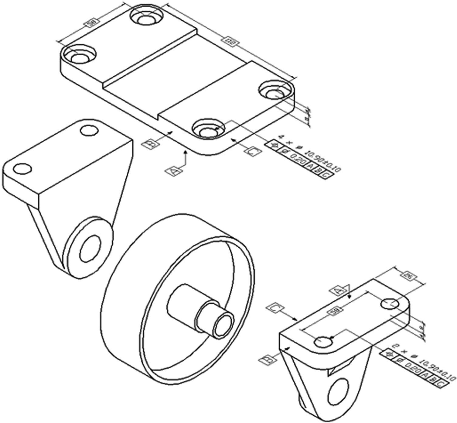
Tolerances of the industrial application example.
The aim of 3D tolerance analysis is to apply the proposed model to evaluate the relative deviation between the supports and the top plate. The bolts used to assemble the support with the top plate have nominal diameter (φB) of 10.00 mm and dimensional tolerance range (±ΔφB) of ±0.58 mm.
Once the relative deviations (Δx, Δy, Δα) of the two supports with respect to the top plate are calculated, both in worst and statistical cases, these can be used to model the stack-up functions of the whole assembly.
To perform the analysis, with the worst-case and the statistical approaches, the equations shown in the previous paragraph have been implemented by means of a MATLAB® macro. The results are shown in Table 1. The statistical approach has been implemented by means of a Monte Carlo simulations with 105 runs; the ranges of Δx, Δy and Δα deviations have been calculated as three times the SD of the obtained PDF.
Tolerance analysis results of the case study.
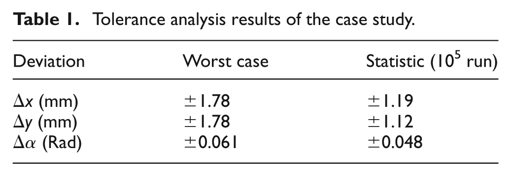
As expected, the deviation’s ranges calculated by the statistical approach are smaller than those calculated by the worst-case approach. The results obtained by the statistical approach show how the deviation along the x-axis is larger than the deviation along the y-axis. This is due to the effect of the interaction between the two bolts that has a greater effect along the transversal direction (y-axis) than along the radial one (x-axis).
Conclusion
This work shows a general model to schematize a clearance joint between the two parts. It takes part of a tolerance analysis model for rigid parts developed to overcome some limits of the literature works. This model links the small kinematic adjustments of the joint to the tolerances applied on the surfaces of the two coupled parts and to the assembly requirements. The general structure of a differential assembly matrix, where a clearance joint is involved, is defined and, then, a criterion to evaluate its small kinematic adjustments is shown. This criterion is based on the evaluation of the boundary surface of the domain of the cumulative effect of the single assembly conditions.
The application of this general model was developed for a typical industrial method to couple with clearance two components of an assembly: a linkage by two bolts. This model permits to evaluate the position deviations between the two joined parts due to the tolerances applied on the components and then to build the transformation matrix needed to model and to solve the tolerance analysis of the assembly. Moreover, this model may be used to design the functional requirements of an assembly since it links the position deviations between the two joined parts and the effective possibility to realize the linkage with the assigned tolerances.
Finally, the proposed model has been applied to a belt drive to solve a 3D tolerance analysis problem. The critical task of the proposed model is the evaluation of the boundary surface of the CAD of the small kinematic adjustments due to the cumulative effect of the single assembly conditions. The application of the proposed model to a linkage by two bolts has evaluated the boundary surface of the CAD by means of geometrical considerations and under the simplified hypothesis to consider the CAD as a circle.
Further research has to be done to develop a general method to evaluate the boundary surface of the domain of the admissible values of the small kinematic adjustments.
Footnotes
Declaration of conflicting interests
The author declares that there is no conflict of interest.