Sage Journals: Discover world-class research

Abstract

In the current study, three-dimensional simulation of an autogenous gas tungsten arc welding of β-titanium alloy (Ti-15V-3Cr-3Sn-3Al) was attempted using the finite element method. Models were developed for continuous current and pulsed current welding at different frequencies (2, 4 and 6 Hz). The transient temperature distributions along the heat-affected zone of the simulated weldments were predicted by considering a moving heat source, the surface heat flux distribution and convectional heat loss in the welded plates. Comparative studies of cooling rates and peak temperatures of the simulated welds between all the generated models were conducted. A realistic temperature at the weld center was also predicted. Results show that both peak temperature and cooling rate exhibit increments with pulsing and also with the increase in frequency up to 4 Hz. Obtained results validated against experimental data showed good agreement.

Keywords

Gas tungsten arc welding continuous current pulsed current peak temperature cooling rates finite element analysis

Introduction

Microstructure of weld fusion zone is of great interest to researchers mainly because it strongly influences joint strength. The microstructural features of welds are dependent on the thermal conditions during welding, which results in varying grain sizes and mechanical properties of welds. Due to the very high-temperature and steep thermal gradients during the process, full control of the solidification rate is not quite possible, and as such, fusion welding is usually accompanied with grain coarsening leading to poor mechanical properties in the weld. Pulsed current gas tungsten arc welding (PC-GTAW)^1–3 is one among the successful alternative methods developed for reduced heat input and grain refinement.^4–6

PC-GTAW involves cycling the welding current at selected regular frequency. The maximum current is selected to give adequate penetration and bead contour, while the minimum is set at a level sufficient to maintain a stable arc.^2,4 This permits arc energy to be used effectively to fuse a spot of controlled dimensions in a short time producing the weld as a series of overlapping nuggets. Advantages include improved bead contours, greater tolerance to heat sink variations, lower heat input requirements, reduced residual stresses and distortion, refinement of fusion zone microstructure and reduced width of heat-affected zone (HAZ).^2,4

One effective, fundamental and inexpensive way to examine whether a certain rate of heat input is sufficient or inadequate to produce a target weld pool profile is through modeling the basic heat transfer phenomena in welding. The basic theory of heat flow was developed by Fourier and was applied by Rosenthal.⁷ He presented the solution of a moving point heat source model, which has been the basis for most subsequent studies of heat flow in welding. Christensen et al.⁸ put the result in dimensionless form and showed that the solution applies to many materials over wide range of heat input. Until the late 1980s, this model was the most popular analytical method for calculating the thermal history of welds. But his assumption of infinite temperature at the heat source and a temperature-independent material, thermal properties lead to serious error in or near the fusion and HAZs. Thereafter, many researchers attempted different assumptions. For instance, Grosh et al.⁹ incorporated temperature dependence of thermal properties, while Tsai¹⁰ used skewed Gaussian heat source and Myers et al.¹¹ discussed in details the effect of these assumptions.

In the late 1960s, with the widespread use of computers, investigators started using numerical methods. Both finite difference and finite element techniques have been applied for the solution of heat transfer equations defining weld thermal cycle. Pavelic et al.¹² suggested distributed heat source and proposed a Gaussian distribution of flux deposited on the surface of workpiece. Krutz and Segerlind¹³ and Friedman¹⁴ combined Pavelic’s disk model with finite element analysis (FEA) and achieved significantly better results than Rosenthal’s model.

Furthermore, many authors have suggested that the heat source should be distributed throughout the molten zone to reflect more accurately the digging action of the arc. Paley and Hibbert¹⁵ followed this approach and proposed a “effective volume heat source” model. Goldak et al.¹⁶ extended Paley and Hibbert’s model by mathematically defining the volumetric heat source dimensions and proposed a non-axisymmetric three-dimensional (3D) heat source model. Goldak’s double ellipsoidal model was more realistic and more flexible than any other proposed model. Both shallow and deep penetration welds could be accommodated as well as asymmetric situations.

Many researchers have worked on modeling and simulation of continuous current (CC)-GTAW with different materials, boundary conditions, heat source models and lot more, but a very few on PC-GTAW. Although experimentally its effects on mechanical and metallurgical properties^4,17–23 have been deeply studied, the effect of different frequencies of PC has been rarely simulated.

Open literature is available for PC-GTAW processes, where the heat input is generally lesser than that of CC welding process. Even though comparison of such welds is generally practiced for highlighting the quality of PC over CC process, such exercise does not usually consider the effect of variation in pulse frequencies. The current study is focused to model the effect of various pulsing frequencies on the thermal profile of metastable β-titanium alloy weldments, for a constant heat input. In the current study, a 3D FE model has been developed to study the temperature distribution along the weldments and validated by experimental data obtained from the open literature⁴ for Ti-15-3 β-titanium alloy.

Gaussian surface heat source model

Welding torch transmits heat over a weld surface, and hence, surface heat flux is closer than Rosenthal’s point heat source where the heat flux is not uniformly distributed. Figure 1 shows the Gaussian distribution of heat flux used by Pavelic to present its disk heat source model. For Gaussian distributed heat source, heat flux (q_i) at certain distance (r_i) from the center of heat source is given by

q_{i} = q_{0} e^{- C {(r_{i} / r_{0})}^{2}}

(1)

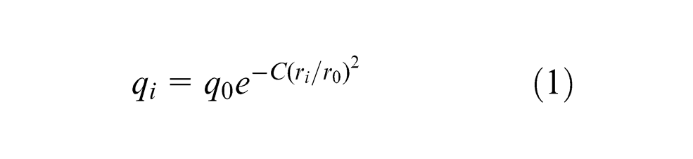
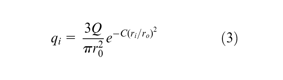
where C is arbitrarily constant. The heat value at the outer radius is 5% of the maximum heat at the center of heat source, and is assumed for calculating C, which comes around 3 and thus

q_{i} = q_{0} e^{- 3 {(r_{i} / r_{o})}^{2}}

(2)

Figure 1.

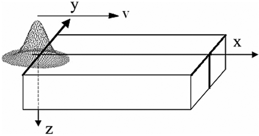
Pictorial representation of bell-shaped welding arc.

Modified version of the above equation for using it in FE model, as suggested by Krutz and Segerlind and Friedman, is

q_{i} = \frac{3 Q}{π r_{0}^{2}} e^{- C {(r_{i} / r_{o})}^{2}}

(3)

where $Q = η VI$ . Equation (3) is used as heat source for the current FE model.

Finite element modeling

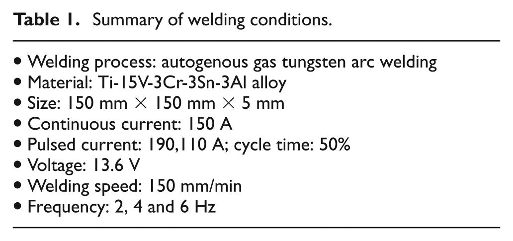
As reported in the literature, two techniques generally used in weld modeling are birth and death technique and the standard technique. The birth and death technique considers growing weld bead with metal deposition, and as such, it is only suitable for non-autogenous process. Being an autogenous weld process, modeling of this study was carried out by standard technique, a rather simple, effective method as it has no additional metal deposition. Welding procedures are summarized in Table 1.

Table 1.

Summary of welding conditions.

• Welding process: autogenous gas tungsten arc welding

• Material: Ti-15V-3Cr-3Sn-3Al alloy

• Size: 150 mm × 150 mm × 5 mm

• Continuous current: 150 A

• Pulsed current: 190,110 A; cycle time: 50%

• Voltage: 13.6 V

• Welding speed: 150 mm/min

• Frequency: 2, 4 and 6 Hz

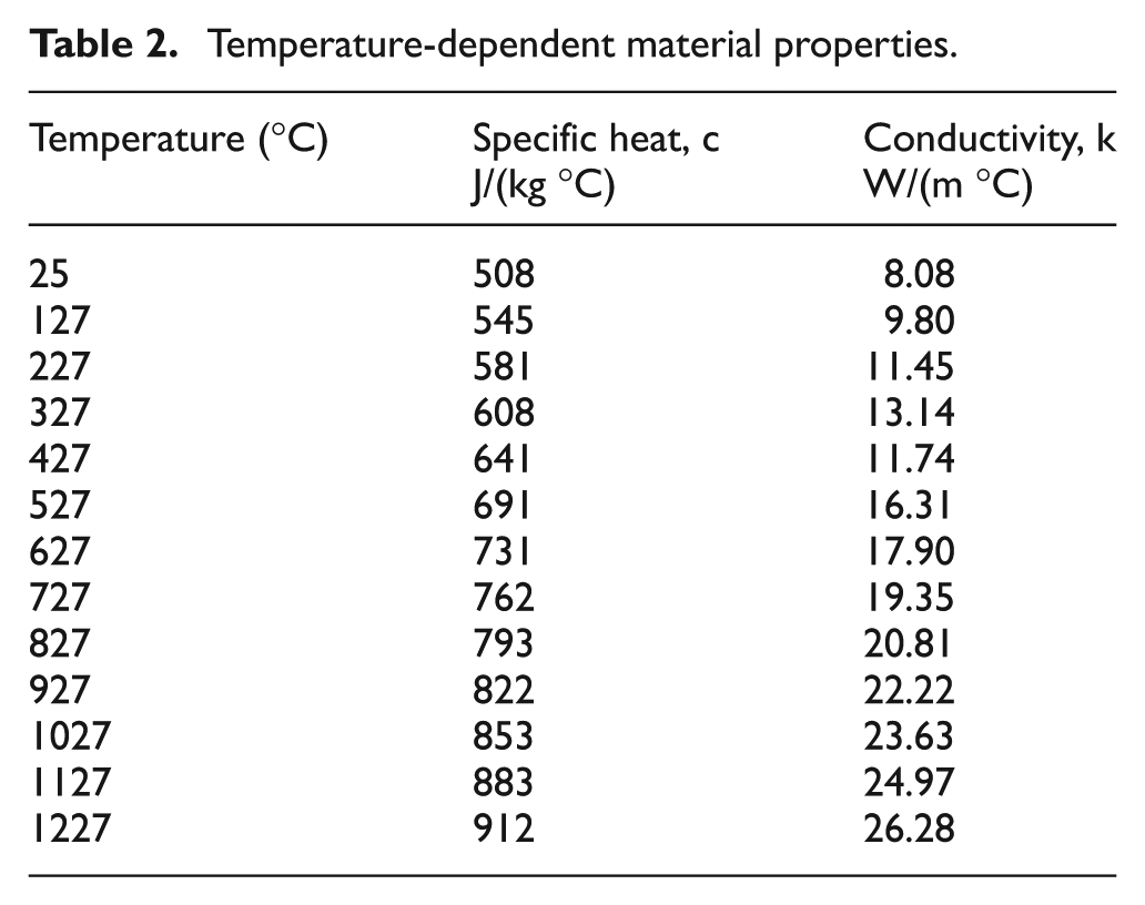
Being symmetrical along the weld centerline, one half of the specimen was considered for modeling. The 3D element of “SOLID Brick 8 node 70” was chosen for the analysis, and mapped meshing was used for the model, by defining the nodes. Finer meshing was done for the near-weld zone, smallest size being 0.2 mm,^24–26 while coarse meshing was done on the remaining areas, as shown in Figure 2. Measured width of weld was 4.2 mm. Temperature-dependent properties, such as thermal conductivity and specific heat of the chosen material, Ti-15-3,²⁷ are shown in Table 2 and were given as input for material model. Gaussian heat source was defined and moved across the weld line with the prescribed speed of 150 mm/min. Finite Element software ANSYS^®28 was used for thermal field simulation, and code enhanced with user subroutines was written in commercial finite element code ANSYS Parametric Design Language (APDL). The heat transfer equations, the boundary conditions and the assumptions made in this model are discussed subsequently.

Figure 2.

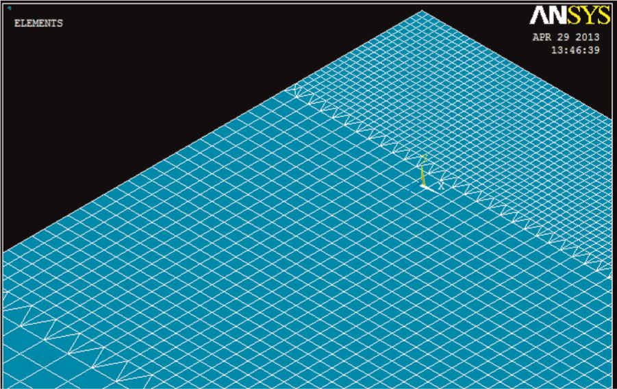
FE mesh of the weld and the plate.

Table 2.

Temperature-dependent material properties.

Temperature (°C)	Specific heat, c J/(kg °C)	Conductivity, k W/(m °C)
25	508	8.08
127	545	9.80
227	581	11.45
327	608	13.14
427	641	11.74
527	691	16.31
627	731	17.90
727	762	19.35
827	793	20.81
927	822	22.22
1027	853	23.63
1127	883	24.97
1227	912	26.28

Heat transfer equations

Mathematical formulation of 3D conduction heat transfer is given by the following differential equation²³ satisfied in some domain R

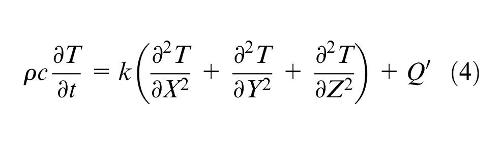
ρ c \frac{\partial T}{\partial t} = k (\frac{\partial^{2} T}{\partial X^{2}} + \frac{\partial^{2} T}{\partial Y^{2}} + \frac{\partial^{2} T}{\partial Z^{2}}) + Q'

(4)

Equation (4) is subjected to the boundary condition, as shown in equation (5)

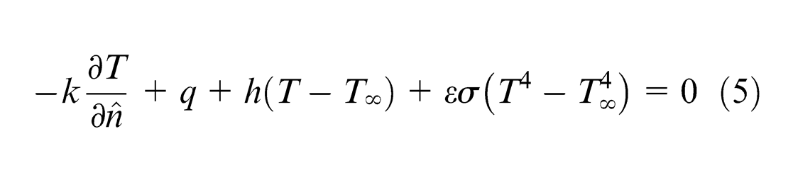
- k \frac{\partial T}{\partial \hat{n}} + q + h (T - T_{\infty}) + ε σ (T^{4} - T_{\infty}^{4}) = 0

(5)

Boundary conditions

The model is subjected to the following boundary conditions:

Initial temperature applied all over the model is $T = T_{\infty}$ for t = 0 where $T_{\infty}$ is the ambient temperature.

The supplied heat flux, $q$ , is assumed to be Gaussian distributed (convection and radiation are not considered to occur over the surface, which receives heat flux.

On all the other surfaces, convection losses are considered.

Assumptions made in the thermal model

All material properties are temperature dependent.

The heat loss due to radiation and conduction through the electrode was accounted in the arc energy transfer efficiency parameter η.²⁹ In the present study, η value for the GTAW process was assumed to be 0.8.

Heat loss due to convection was considered on all the surfaces, as referred in the boundary conditions.

Effect of shielding gas flow on the heat losses was not considered.

Being a complex phenomenon, weld pool convection was compensated by multiplying the conductivity with a factor (between 8 and 10),³⁰ when the temperature exceeds the liquidus temperature.

Conductivity should be increased just below the melting point to account for increased conductivity due to stirring effect in molten metal.

Results and discussion

For calculating heat input (Q) for the PC process, mean current was calculated using equation (6)

I_{m} = {(I_{p} \times t_{p}) + (I_{b} \times t_{b})} / t_{T}

(6)

In order to have a better understanding of the effect of various PC frequencies used and also to have a comparative study of the advantages of the PC over that of CC, the heat input should be made constant for both. While all other weld parameters are kept constant, the peak current, the base current, the time on peak pulse and the time on base current were so chosen that the mean current for PC-GTAW would be the same as that of the current parameters used in CC-GTAW.

The time–temperature plots (Figure 3) were obtained for each model (CC, 2, 4 and 6 Hz) at 9 mm distance from the weld center. Weld center temperatures were predicted for each model, which could be really challenging during in situ temperature measurements using thermocouples. Peak temperatures obtained during the simulation of the various weld parameters of CC and PC are listed in Table 3. As the heat source moves along the weld line, thermal profile of the weld plates changes continuously. Figure 4(a)–(c) shows such a time variant thermal profiles for CC weld model at 10, 24 and 40 s, respectively.

Table 3.

Peak temperatures and weld center temperature.

	Peak temperature		Predicted weld center temperature (°C)
	Experiment¹¹ (°C)	Model (°C)	Predicted weld center temperature (°C)
CC	900	965	2644
2 Hz	940	1012	2632
4 Hz	1230	1034	2636
6 Hz	920	988	2638

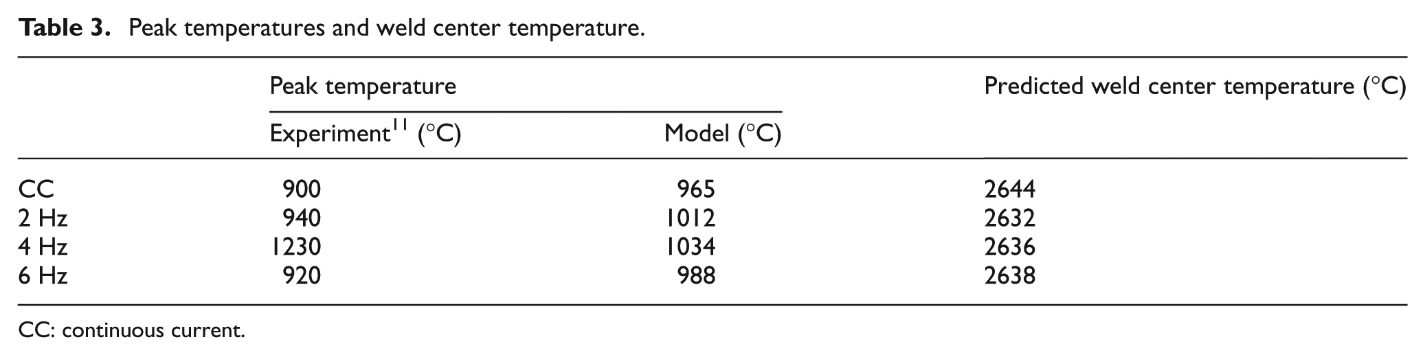
CC: continuous current.

Figure 3.

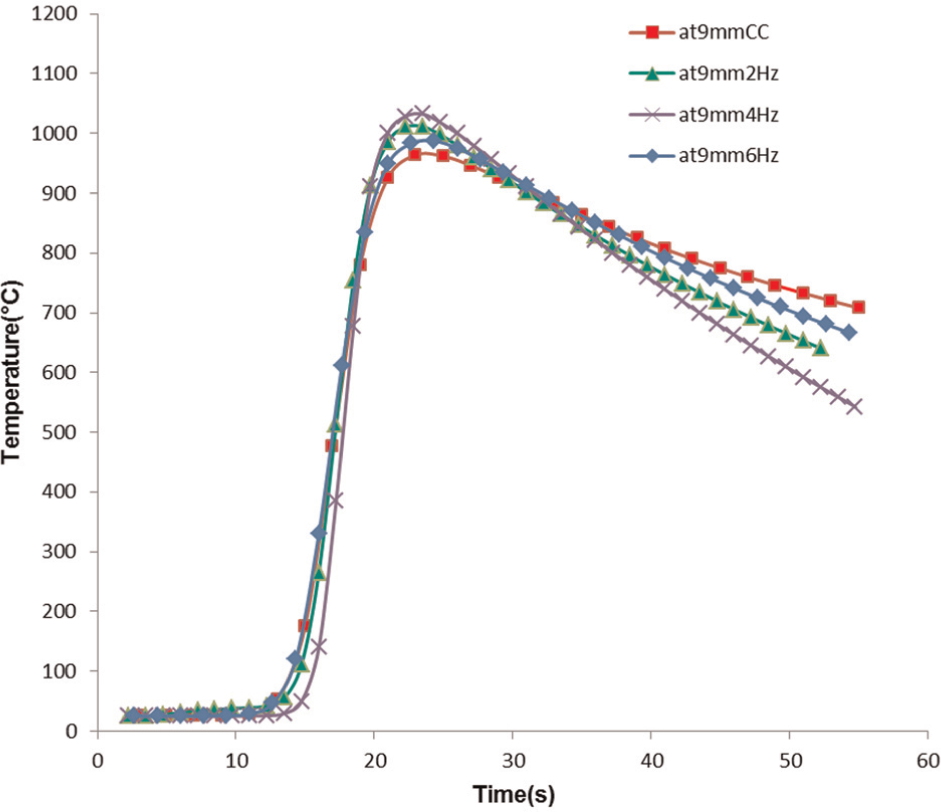
Simulated plots of thermal cycles for different conditions of PC and CC.

Figure 4.

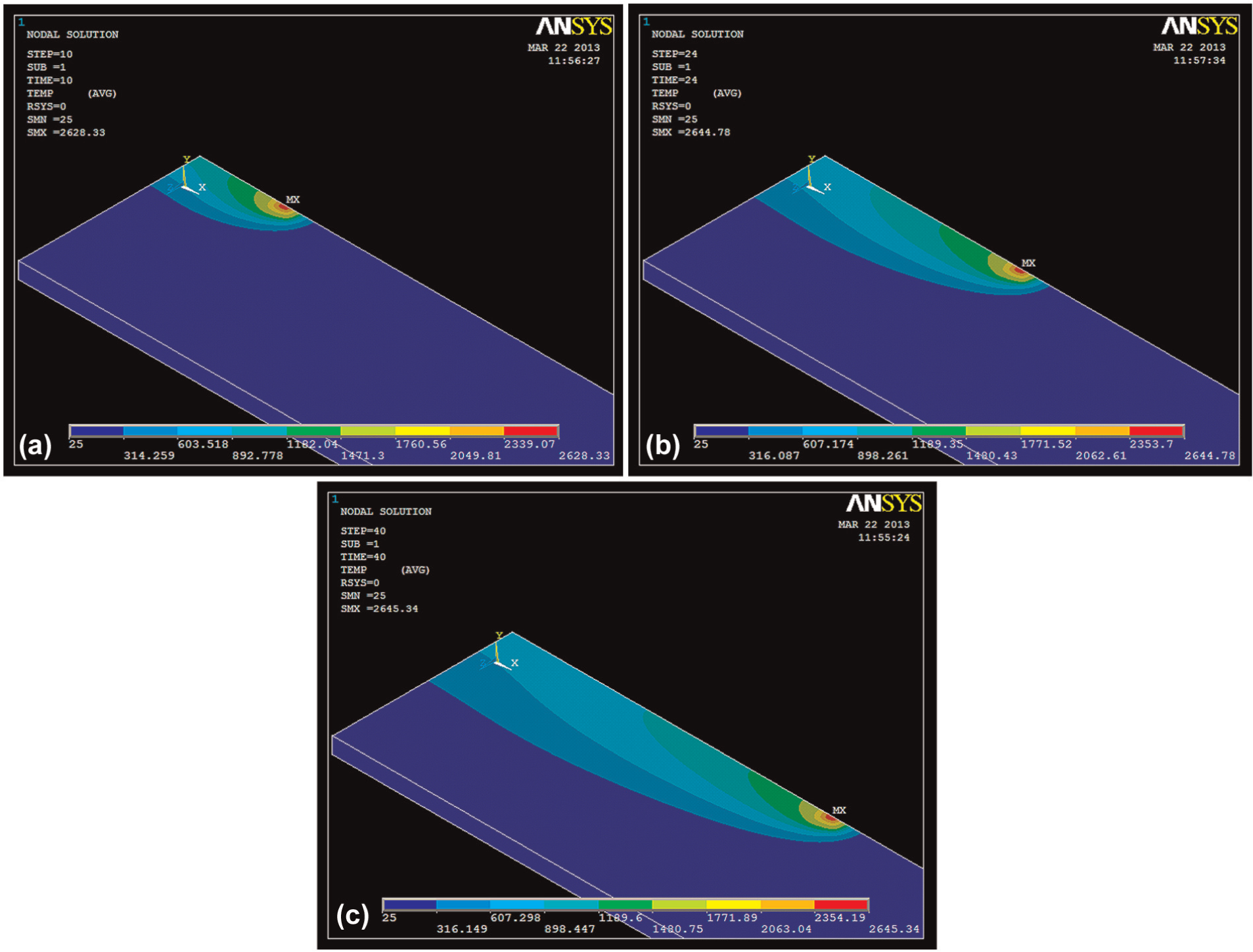
Thermal profile of CC model at different positions: (a) 10s, (b) 24s and (c) 40s.

Peak temperature

Table 3 indicates that the peak temperature for 2 Hz PC is 1012 °C while that for CC is 965 °C, with a difference of around 47 °C. The peak temperature for 4 Hz PC is 1034 °C and 22 °C higher than that of 2 Hz PC weld, while the peak temperature for 6 Hz PC weld is 24 °C and 46 °C lesser than that of 2 and 4 Hz PC welds, respectively. This goes in par with the same trend seen during the experiments, and it could be attributed to the effect of low thermal diffusivity of β-titanium alloy (D = 3.44 × 10⁻⁶ m²/s at room temperature (RT)), same weld traverse speed (2.5 mm/s) on all the frequencies and also the pulsed frequency (n), as discussed in the published literature.⁴

Furthermore, the deviation over the entire window of the parameters used in the simulated temperature values over that of the experiments was calculated to be less than 8%. This small and consistent deviation could be attributed to the assumptions made while developing the model, namely, effect of radiation and the effect of argon shielding (backup and trailing gas) over the fusion zone were not considered in the model. Furthermore, the convection heat transfer coefficient, which depends on material as well as on the surrounding, was assumed, which could be slightly different from the real value.

Cooling rate

Higher peak temperature enhances large thermal gradients and increased convection leads to higher cooling rates. Cooling rates from simulated thermal plots were compared with that of experiments. The cooling rates of all the PC welds were found to be higher than that of the CC welds, similar to the experimental results. Furthermore, as frequency increased to 4 Hz, cooling rate also increased to 15.6 °C/s, an increment of 3 °C/s, which is almost consistent with previous increment of 4 °C/s between CC and 2 Hz PC. The decrease in the cooling rate of 6 Hz PC weld (10.55 °C/s) could be attributed to the low peak temperature compared to 2 and 4 Hz PC weldments, as cooling rate depends on thermal gradient.

It was observed that deviation between simulated and experimental results were higher for 4 Hz model compared to other cases. Reason for this inconsistent behavior at 4 Hz is not clear at present. But the literature suggests that it may be due to the HAZ receiving sensible heat from the moving torch in a manner that accumulates the heat, and hence, it increases the peak temperature, which also affects the cooling rate.⁴ To achieve this behavior in the model, a perfect combination of various parameters within a chosen window is must. But in the model, other than the precise experimental values, remaining parameter values were assumed. The combined effect of all those assumptions probably resulted in the current deviation measured in the simulated model and the experimental values. Also simulated thermal history was plotted for 60 s in simulation and for 150 s during experiment. As thermal gradient is decreasing after the completion of the weld (i.e. after the arc has extinguished at the far end of the weld line), the cooling rate also decreases, which was not considered in the model.

Conclusion

The transient temperature profile and the cooling rate in β-titanium alloy during CC-GTAW and PC-GTAW processes were successfully simulated and verified with experimental results.

The model is particularly suitable for the prediction of the weld centerline thermal conditions, thus eliminating the challenges with real-time measurement with thermocouple.

For a chosen constant heat input, PC as well as an increase in pulse frequency up to 4 Hz resulted in increment of peak temperature and cooling rate.

Simulated and experimental results compared fairly well with a variation of only 8% for the peak temperatures.

Footnotes

Appendix 1 Declaration of conflicting interests

The authors declare that there is no conflict of interest.

Funding

This research received no specific grant from any funding agency in the public, commercial or not-for-profit sectors.

References

Kou

. Nucleation mechanisms and grain refining of weld metal. Weld J1986; 65: 305s–313s.

Madhusudhan Reddy

Gokhale

Prasad Rao

. Optimization of pulse frequency in pulsed current gas tungsten arc welding of aluminium–lithium alloy sheets. J Mater Sci Technol1998; 14: 61–66.

Kumar

Sundarrajan

. Optimization of pulsed TIG welding process parameters on mechanical properties of AA 5456 Aluminum alloy weldments. Mater Design2009; 30: 1288–1297.

Balachandar

Sarma

Pant

. Microstructure and mechanical properties of GTA welded Ti-15-3 beta titanium alloy. Metall Mater Trans A2009; 40: 2685–2693.

Moldovan

Popescu

. The grain refinement of 6063 aluminum using Al-5Ti-1B and Al-3Ti-0.15C grain refiners. JOM: J Min Met Mat S2004; 56: 59–61.

Chern

T-S

Tseng

K-H

Tsai

H-L

. Study of the characteristics of duplex stainless steel activated tungsten inert gas welds. Mater Design2011; 32(1): 255–263.

Rosenthal

. The theory of moving sources of heat and its application to metal treatments. Trans Am Inst Min Metall Pet Eng1946; 43(11): 849–866.

Christensen

Davies

Gjermundsen

. Distribution of temperature in arc welding. Br Weld J1965; 12: 54–75.

Grosh

Trabant

Hawkins

. Temperature distribution in solids of variable thermal properties heated by moving heat sources. Q Appl Math1955; 13(2): 161–167.

10.

Tsai

. Modelling of casting and welding processes, Proc. Conf., Henniker, NH, 31 July–5 August 1983. Warrendale, PA: TMS-AIME, pp. 329–341, 1984.

11.

Myers

Uyehara

Borman

. Fundamentals of heat flow in welding (Welding Research Council bulletin), vol. 123. New York: Welding Research Council, 1967.

12.

Pavelic

Myers

Tanbakuchi

. Experimental and computed temperature histories in gas tungsten arc welding thin plates. Weld J1969; 48(7): 295s–305s.

13.

Krutz

Segerlind

. Finite element analysis of welded structures. Weld J1978; 57: 211s–216s.

14.

Friedman

. Thermomechanical analysis of the welding process using the finite element method. J Press Vess: T ASME1975; 97(3): 206–213.

15.

Paley

Hibbert

. Computation of temperatures in actual weld design. Weld J1975; 54: 385s–392s.

16.

Goldak

Chakravarthi

Bibby

. A new finite element model for welding heat sources. Metall Trans B1984; 15: 299–305.

17.

Fanous

IFZ

Younan

MYA

Wifi

. 3-D finite element modeling of the welding process using element birth and element movement techniques. J Press Vess: T ASME2003; 125: 144–150.

18.

Jantre

Ghosh

. Prediction of weld quality in pulsed current GMAW process using artificial neural network. Sci Technol Weld Joi2004; 9(3): 253–259.

19.

Janaki Ram

Venugopal Reddy

Prasad Rao

. Improvement in stress rupture properties of Inconel 718 GTA welds using current pulsing. J Mater Sci2005; 40: 1497–1500.

20.

Balasubramanian

Jayabalan

Balasubramanian

. Effect of pulsed gas tungsten arc welding on corrosion behavior of Ti–6Al–4V titanium alloy. Mater Design2008; 29: 1359–1363.

21.

Senthil Kumar

Balasubramanian

Babu

. Effect of pulsed current GTA welding parameters on the fusion zone microstructure of AA6061 aluminum alloy. Met Mater Int2007; 13: 345–351.

22.

Balasubramanian

Senthil Kumar

Sanavullah

. Influences of pulsed current tungsten inert gas welding parameters on tensile properties of AA6061 aluminium alloy. Mater Design2007; 28: 2080–2092.

23.

Lothongkum

Chaumbai

Bhandhubanyong

. TIG pulse welding of 304L austenitic stainless steel in flat, vertical and overhead positions. J Mater Process Tech1999; 90: 410–414.

24.

Darmadi

Tieu

Norrish

. A validated thermal model of bead-on-plate welding. Heat Mass Transfer2012; 48(7): 1219–1230.

25.

Capriccioli

Frosi

. Multipurpose ANSYS FE procedure for welding processes simulation. Fusion Eng Des2009; 84: 546–553.

26.

Lundback

. FE modelling and simulation of welding of aerospace components. PhD Thesis, Department of Applied Physics and Mechanical Engineering, Luleå University of Technology, Luleå, 2003.

27.

Boyer

Welsch

Colings

. Materials properties handbook: titanium alloys. Materials Park, OH: ASM International, 1994, p.901.

28.

Ansys, Inc. Theory reference. Pittsburgh: Ansys Inc., 2007.

29.

Stenbacka

Choquet

Hurtig

. Review of arc efficiency values for gas tungsten arc welding. In: Intermediate meeting, Berlin, April 2012, http://hv.diva-portal.org/smash/get/diva2:523654/FULLTEXT01.pdf

30.

Ericsson

. Simulation of robotic TIG-welding. PhD Thesis, Department of Technology, University of Trollhättan, Trollhättan, 2003.

Three-dimensional finite element simulation of gas tungsten arc welding for β-titanium alloy

Abstract

Keywords

Introduction

Gaussian surface heat source model

Finite element modeling

Heat transfer equations

Boundary conditions

Assumptions made in the thermal model

Results and discussion

Peak temperature

Cooling rate

Conclusion

Footnotes

Appendix 1

Declaration of conflicting interests

Funding

References