Modelling and experimental analysis of surface roughness in spherical grinding

Abstract

A new method for predicting the surface roughness in spherical grinding was developed. Spherical grinding typically uses a cup grinding wheel containing segmented abrasive blocks that continually engage the surface of the sphere workpiece during grinding. In this study, the trajectory of the abrasive grain, undeformed chip thickness, and the grinding mechanism are considered separate from the surface grinding process. Therefore, the traditional method used to determine surface roughness based on surface grinding cannot be applied to predict the surface roughness in spherical grinding. A new analytical spherical surface roughness model was developed based on chip thickness, and the effect of overlapping of triangle grooves produced by multiple abrasive grains was considered to improve the precision of the roughness model. The process parameters that affect spherical surface roughness are theoretically analysed and experimentally studied. Comparison of the experimental results with the predicted results derived from the developed roughness model validates the proposed model and demonstrates the effects of the fundamental factors on surface roughness in spherical grinding.

Introduction

The ball valve, which can resist high temperatures (>500 °C), high pressure (>30 MPa), corrosion, and wear, is the core component of fluid and gas control devices used in natural gas transmission, petroleum chemical engineering, steel smelting, coal liquefaction, and nuclear power plants. To fulfil the stringent requirements of a harsh working environment, the ball of the valve, ranging from 200 to 1000 mm in diameter, is typically composed of a 304 stainless steel base material with 0.4–0.6 mm of thick thermal spray-coated tungsten carbide (WC) in a Co matrix surface layer to achieve high hardness (Rockwell hardness > 65) and wear resistance. The spherical surface of the ball must be precise. In many situations, the sphericity error of the sphere is required to be less than 0.008 mm, and the spherical surface roughness (R_a) should be less than 0.1 µm. The high-precision grinding of a large-area and high-hardness spherical coating is one of the key techniques used in ball valve manufacturing.

Grinding keeps as one of the most crucial and feasible machining techniques because it produces hard materials characterised by super form accuracy and surface integrity. ¹ Numerous studies have been undertaken to evaluate the surface roughness of a grinding workpiece. Several analytical models have been built in predicting the surface roughness of a workpiece from the grinding process. Hecker and Liang. ² analytically derived a model of arithmetic mean surface roughness from a probabilistic undeformed chip thickness model and discovered a simple expression that relates surface roughness with chip thickness, which was verified by a cylindrical grinding experiment. Stepien ³ proposed a probabilistic model of the grinding process by considering the random arrangement of grain vertices on the wheel active surface. The probability of contact between the grains and the work material, the undeformed chip thickness are described in the grinding zone. Agarwal and Rao developed a new analytical surface roughness model incorporating the effects of overlapping of hemisphere-shaped grooves^4,5 and parabolic-shaped grooves ⁶ to predict surface roughness based on the chip thickness probability density function (pdf). These developed models have been validated by the results of ceramic grinding experiments. Chen and Rowe ⁷ studied the roughness model during spark-out by considering the effects of machine stiffness, system deflection, wheel sharpness, and plastic deformation. Zhou and Xi ⁸ proposed a new method to predict surface roughness by considering the random distribution of grain protrusion heights instead of using the average value of grain protrusion heights, as traditional models have used. The results indicated that this method effectively improved the accuracy of roughness prediction.

All of these models were developed based on plane grinding using a straight wheel. Spherical grinding is a closed grinding method that allows an abrasive to continually engage the surface of workpiece while grinding. The abrasive grain trajectory, undeformed chip thickness, and the grinding mechanism are all different from those in the plane grinding process. The existing surface roughness models all pertain to plane grinding and cannot be applied to curve grinding. A spherical surface roughness model has not been analytically researched until now.

In this article, the sphere generation mechanism used in spherical grinding is first introduced. A new analytical surface roughness model was developed by considering the overlapping of triangle-shaped grooves produced by multiple abrasive particles. The assumed triangle-shaped grooves simplify the analysis and are close to reality, which can be concluded by observing the shape of the abrasive particles using a scanning electron microscope. The spherical grinding experiment setup and procedure are also introduced. The spherical surface roughness is calculated based on the roughness model. The theoretical roughness values are compared with those of the experimental results. The impact of the grinding parameters on spherical surface roughness is then discussed based on both the experiments and roughness modelling.

Mathematical model of surface roughness

Sphere generation mechanism used in spherical grinding

The schematic illustration of sphere grinding by using a cup wheel is displayed in Figure 1. The workpiece, which is the ball of the valve, is fixed in a special fixture. One end of the fixture is clamped by a chuck, and the other is supported by a live centre in the spindle of tailstock. The workpiece can rotate with the fixture around the centre line of the workpiece spindle, which is the Y axis. The cup wheel is connected with a motorised spindle that is mounted in the sliding headstock. The diameter of the cup wheel is large enough for the wheel to grind the entire spherical surface of the workpiece. The abrasive wheel blocks are installed circumferentially and evenly in the body fringe of the cup wheel. This type of wheel structure facilitates the cooling and disposal of chips and reduces the grinding force. The sliding headstock is powered by a servo motor along the linear guide to allow the wheel to complete the feed movement. The workpiece spindle and the tailstock spindle are all moveable and can be numerically controlled to move synchronously along the Y axis. The centre lines of the cup wheel and workpiece spindle and the tailstock spindle vertically intersect at sphere centre O. During the sphere grinding process, the workpiece rotates around the Y axis, and the cup wheel rotates around the X axis and feeds automatically in the X direction, as illustrated in Figure 1.

Figure 1.

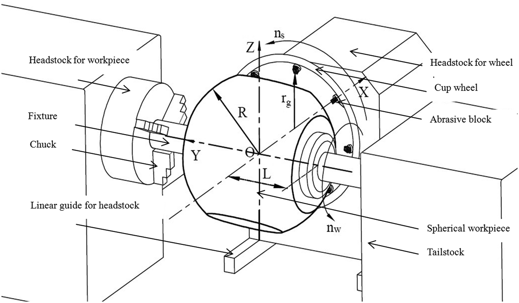
Schematic illustration of the sphere grinding machine.

Model development

Grinding is commonly regarded as the most complex material removal process compared with other machining processes, primarily because of the complex grinding mechanism of the abrasive. ⁹ The cutting edges are randomly distributed on the wheel surface and vary in shape and size, which results in random variations in the abrasive grain protrusion heights. Considering the complexity of the grinding process, the following assumptions were established:

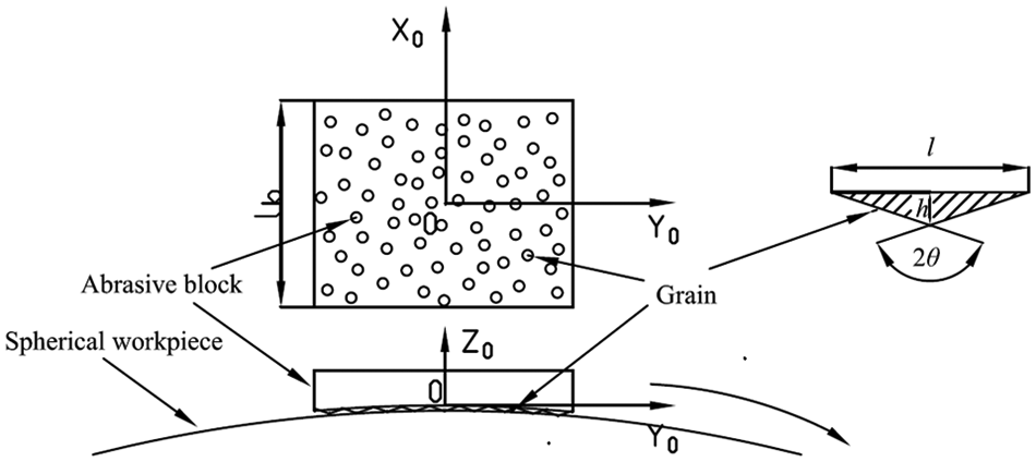
1. The grains are randomly distributed across the wheel surface and are approximately cone shaped with a coning angle of 2θ.

2. The profiles of grooves produced by the grains and located in the ground surface are triangle shaped and defined by the depth of the groove, h, which equals the undeformed chip thickness.

3. Only the chip formation stage of the grinding process is considered.

Figure 2 displays the distribution of the grinding wheel grains in the X₀Y₀ coordinate system. The coordinate X₀ indicates the random position of a grinding grain along the width direction of the wheel block. The coordinate X₀ can be regarded as having a uniform distribution. ¹⁰ Thus, the pdf of X₀ can be expressed as

$$f(x)=\frac{1}{l_b},0⩽x⩽l_b$$

(1)

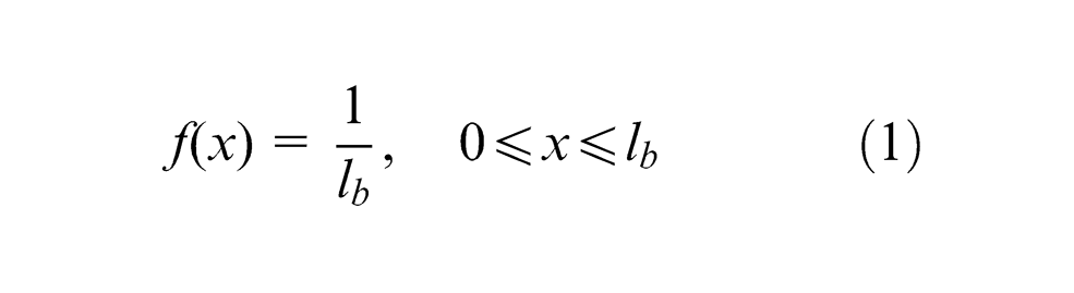
where $l_b$ is the wheel block width.

Figure 2.

The contact between the grinding wheel and workpiece.

A pdf can be applied to represent the distribution of undeformed chip thickness generated by various grain heights when the sphere is ground under certain grinding conditions because of the varying size and height of the grains. This distribution is generally described using a Rayleigh pdf proposed by Alawi and Younis. ¹¹ In the sphere grinding process, undeformed chip thickness is equal to the groove depth generated by the cutting of effective abrasive grain on the ground surface. Therefore, the spectrum of generated groove depth can be assumed to have the same mathematical distribution. The Rayleigh pdf of groove depth f(h) is given by

$$f(h)=\{\begin{array}{cc}\multicolumn{1}{c}{}& \frac{h}{{\sigma }^2}{e}^{-\frac{h^2}{2{\sigma }^2}},h⩾0\hfill \\ \multicolumn{1}{c}{}& 0,h<0\hfill \end{array}$$

(2)

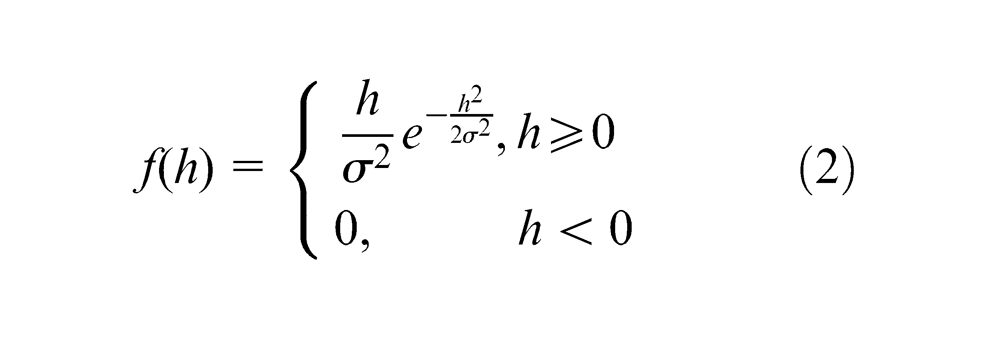
where σ is a parameter that completely defines the Rayleigh pdf and depends on factors such as the grinding conditions, the microstructure of the grinding wheel, and workpiece material.

The Rayleigh distribution is similar to a logarithmic standard distribution, ¹² which is used to describe the chip thickness distribution. However, the Rayleigh pdf has the advantage of being uniquely defined by only one parameter, σ. In this study, the Rayleigh distribution was used for formula derivation.

The random distribution of grains in the wheel is primarily caused by the manufacturing process and structure of the grinding wheel. The space distribution of grains on the grinding wheel surface is illustrated in Figure 2.

At any cross-section along the axial direction of X₀, displayed in Figure 2, assume x_i and x_i+1 are the positions of two grooves generated by grains on the ith and (i+ 1)th columns exhibited in Figure 3. The grains are randomly distributed on the wheel surface and, therefore, x_i and x_i+1 are independent random variables. The centre-to-centre distance φ between two grains is given by $l_1=x_{i+1}-x_i$ , which can be described as the extent of overlapping of triangle-shaped grooves.

Figure 3.

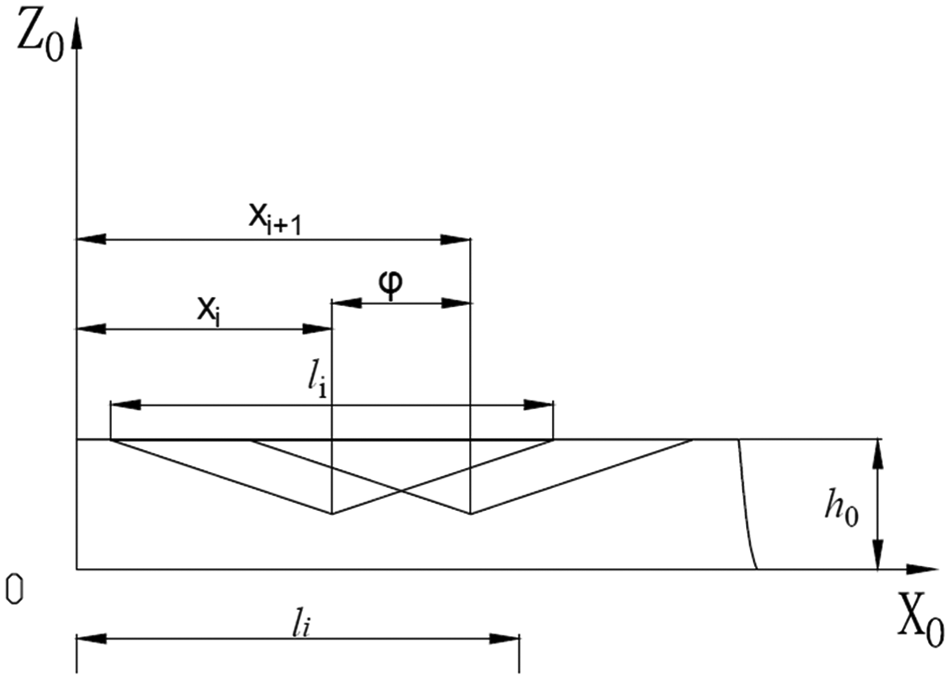
Cross-sectional view of the distance between the successive grooves.

The expected distance of φ can be derived^4,6 as

$$E\left(\phi \right)=\frac{l_i}{3}$$

(3)

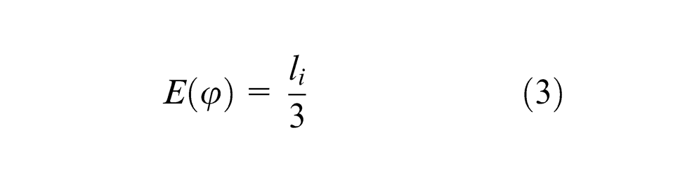
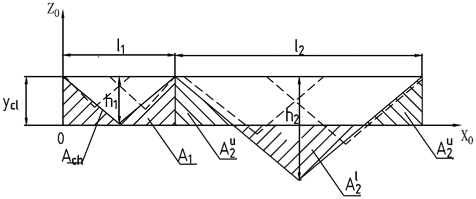
where l_i is the width of the groove located on the workpiece surface. Therefore, the expected value of the distance between the centres of two overlapping grooves along the direction X₀ is one-third times the groove width. Therefore, the overlapping profile generated by abrasive grains with the same height is displayed in Figure 4. In Figure 4(a), considering the region between the two vertical lines, S₁ is the remaining section area produced by one individual grain. $S{\prime }_1$ is the remaining section area considering the overlapping of grooves. The overlap factor k₁ is defined as the area residual factor caused by overlapping and can be expressed as

$$k_1=\frac{{S\prime }_1}{S_1}=0.33$$

(4)

Figure 4.

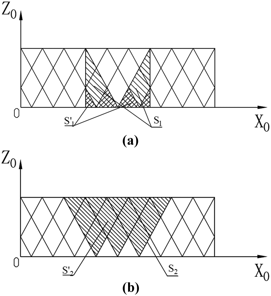
Overlapping profile generated by grain grooves. (a) diagram of overlap factor k1 and (b) diagram of overlap factor k2.

In Figure 4(b), S₂ is the cut section area produced by one individual grain, ${S\prime }_2$ is the cut section area produced by three individual grains considering the overlapping of grooves. The area overlapping factor k₂ is defined as

$$k_2=\frac{{S\prime }_2}{3S_2}=0.7$$

(5)

The surface roughness, R_a, can be calculated by using equation (6). R_a is the mean derived from the absolute values of the vertical deviation of each sampling point on the roughness profile to the centre line in the range of sampling length r.

$$R_a=\frac{1}{r}\underset{0}{\overset{r}{\int }}|y-y_{\mathrm{cl}}|\mathrm{dr}$$

(6)

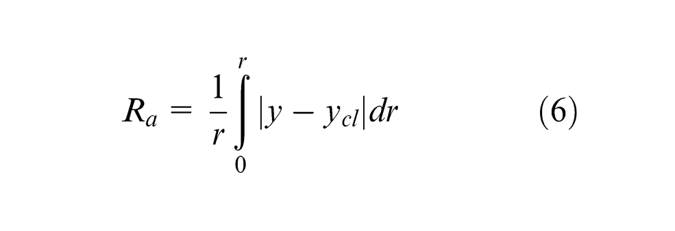
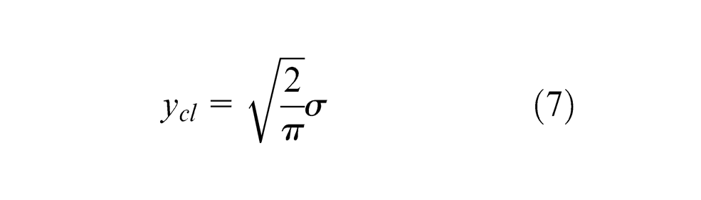
in which y_cl represents the position of the centre line, which is illustrated in Figure 5.

Figure 5.

Theoretical profile generated by multiple abrasive grain grooves.

The position of this line can be calculated using equation (7) ²

$$y_{\mathrm{cl}}=\sqrt{\frac{2}{\pi }}\sigma$$

(7)

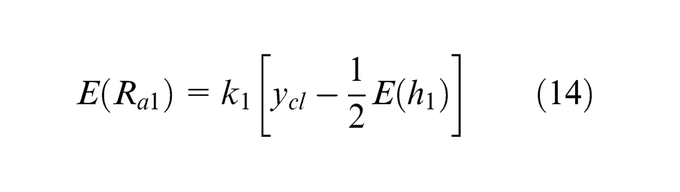
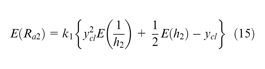
Among all of the grooves generated, two types of groove can be distinguished depending upon whether the depth of the grooves is either less or greater than the centre line, y_cl. Based on these two types of groove, the total expected value of surface roughness can be expressed using equation (8)

$$E\left(R_a\right)=p_{1}E\left(R_{a1}\right)+p_{2}E\left(R_{a2}\right)$$

(8)

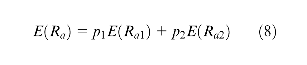
where E(R_a1) is the expected roughness value on condition that the depth of the grooves is less than y_cl. E(R_a2) is the expected roughness value on condition that the depth of the grooves is greater than y_cl. Hence, the following can be deduced: ² $p_1=1-e^{-1/\pi }$ and $p_2=e^{-1/\pi }$ .

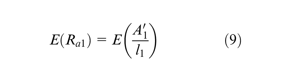
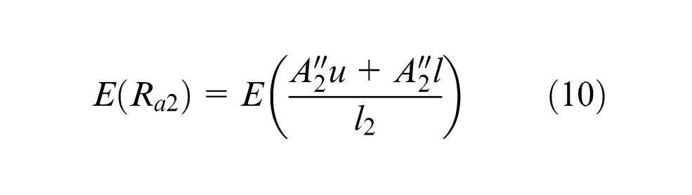
The surface roughness can be calculated using the sum of the areas between the profile and the centre line divided by the sampling length. Based on Figure 5, two expected roughness values can be calculated as

$$E\left(R_{a1}\right)=E\left(\frac{{A\prime }_1}{l_1}\right)$$

(9)

$$E\left(R_{a2}\right)=E\left(\frac{{A″}_{2}u+{A″}_{2}l}{l_2}\right)$$

(10)

where ${A\prime }_1$ , ${A″}_{2}u$ , and ${A″}_{2}l$ are considered the overlapping effects of $A_1$ , $A_2^u$ , and $A_2^l$ . Based on Figure 5, the expected value of the area on condition that the depth of the grooves is less than y_cl can be written as

$$E\left({A\prime }_1\right)=\tan \left(\theta \right)k_1[2y_{\mathrm{cl}}E\left(h_1\right)-E\left(h_1^2\right)]$$

(11)

Similarly, the expected area for the groove characterised by a depth that is greater than y_cl can be written as

$$E\left({A″}_{2}u\right)=\tan (\theta )k_1{y}_{cl}^2$$

(12)

$$E\left({A″}_{2}l\right)=\tan \left(\theta \right)k_1\left[y_{cl}^2+E\left(h_2^2\right)-2y_{cl}E\left(h_2\right)\right]$$

(13)

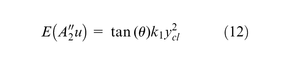
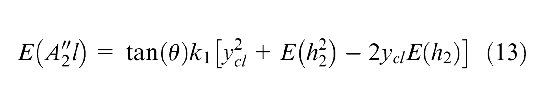
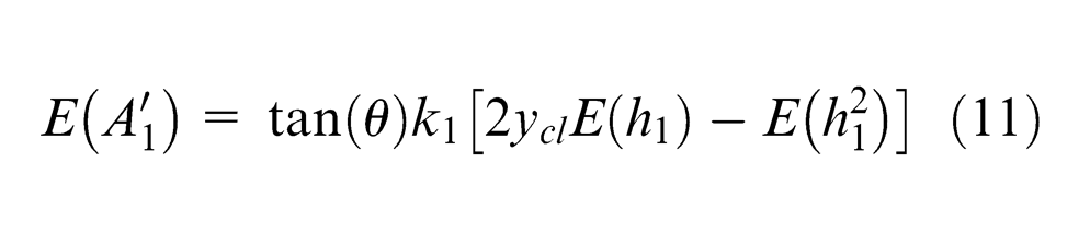
By substituting equations (11)–(13) into equations (9) and (10), the equation becomes

$$E\left(R_{a1}\right)=k_1[y_{\mathrm{cl}}-\frac{1}{2}E\left(h_1\right)]$$

(14)

$$E\left(R_{a2}\right)=k_1\{y_{\mathrm{cl}}^{2}E\left(\frac{1}{h_2}\right)+\frac{1}{2}E\left(h_2\right)-y_{\mathrm{cl}}\}$$

(15)

In addition, the following results are deduced ²

$$\begin{array}{cc}\multicolumn{1}{c}{}& E\left(h_1\right)=\frac{\underset{0}{\overset{y_{\mathrm{cl}}}{\int }}{h}_{1}f\left(h_1\right)d{h}_1}{p_1}=0.52\sigma \hfill \\ \multicolumn{1}{c}{}& E\left(h_2\right)=\frac{\underset{y_{\mathrm{cl}}}{\overset{\infty }{\int }}{h}_{2}f\left(h_2\right)d{h}_2}{p_2}=1.53\sigma \hfill \\ \multicolumn{1}{c}{}& E\left(\frac{1}{h_2}\right)=\frac{\underset{y_{\mathrm{cl}}}{\overset{\infty }{\int }}\frac{1}{h_2}\frac{h_2}{{\sigma }^2}{e}^{-\frac{h_2^2}{2{\sigma }^2}}d{h}_2}{p_2}=\frac{0.73}{\sigma }\hfill \end{array}$$

(15)

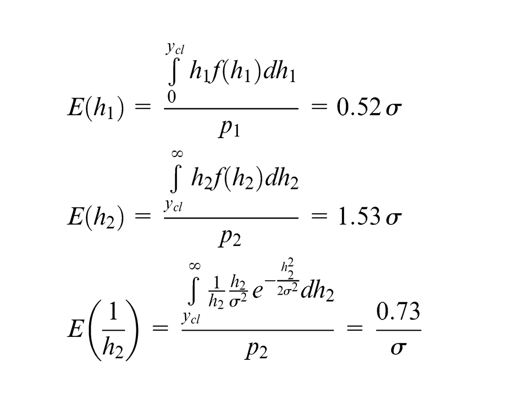
By substituting equations (14) and (15) into equation (8), including these results, the expected value of surface roughness can be derived as

$$E\left(R_a\right)=0.463k_1\sigma$$

(16)

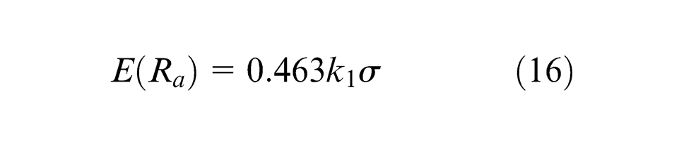
Equation (16) demonstrates the relationship between surface roughness and $\sigma$ .

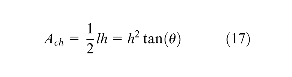
The average chip cross-section A_ch with a triangle shape and an internal angle of 2θ (Figure 5) can be expressed as

$$A_{\mathrm{ch}}=\frac{1}{2}\mathrm{lh}=h^2\tan \left(\theta \right)$$

(17)

The expected value of the total area of engagement, which is projected to a plane perpendicular to the movement direction of the grain in the grinding zone, is the combination of all of the areas engaged by each individual active grain, which can be expressed as

$$E\left({A\prime }_{\mathrm{total}}\right)=N_{d}E\left({A\prime }_{\mathrm{ch}}\right)=k_2{N}_{d}E\left(A_{\mathrm{ch}}\right)=k_2{N}_d\tan \left(\theta \right)E\left(h^2\right)$$

(18)

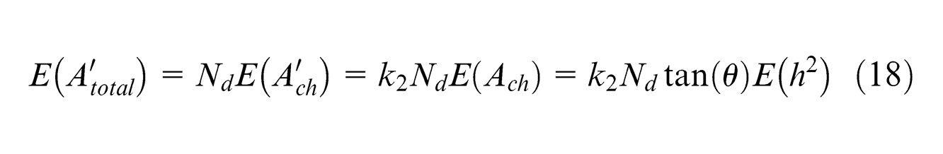
where k₂ is the area overlapping factor, and the instantaneous number of active cutting edges is

$$N_d=S_d{C}_d$$

(19)

where S_d is the actual contact area of the grinding wheel block and C_d is the dynamic cutting edge density.

$$S_d\cong l_a{l}_b$$

(20)

where l_a and l_b are the length and width of the grinding wheel piece, respectively.

Considering the effect of increasing the number of grinding wheel blocks, the expected value of the total area can be expressed as

$$E\left(A_{\mathrm{total}}\right)=N_{s}E\left({A\prime }_{\mathrm{total}}\right)$$

(21)

Based on the fact that the material removal amount is conserved, the total projected engaged area multiplied by the linear velocity of the wheel equals the material removal rate (MRR) (Figure 1)

$$\text{MRR}=a_0\frac{4\pi R^2-4\pi R(R-L)}{2\pi }\frac{2\pi n_w}{60}=2a_0\mathrm{RL}\frac{2\pi n_w}{60}$$

(22)

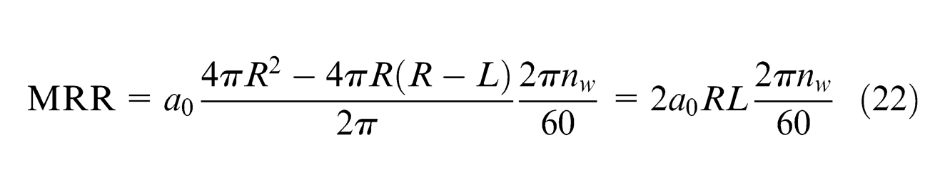
Therefore

$$E\left(A_{\mathrm{total}}\right)r_g\frac{2\pi n_s}{60}=2a_0\mathrm{RL}\frac{2\pi n_w}{60}$$

(23)

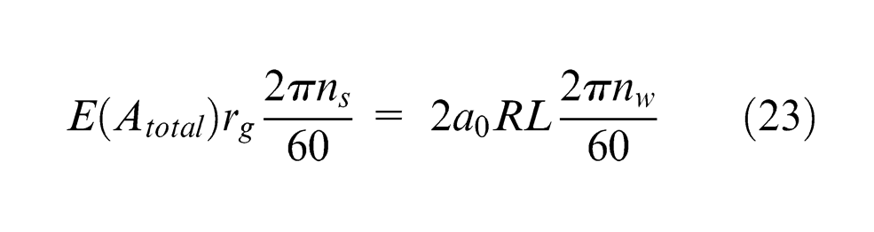
where n_s is the wheel speed, n_w is the workpiece speed, and a₀ is the feed rate of the grinding wheel (i.e. feed per workpiece revolution).

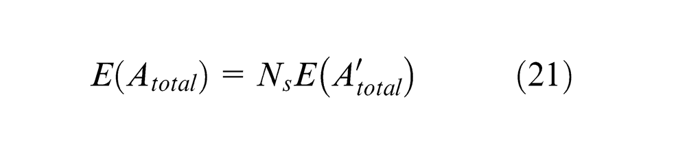
The relationship between undeformed chip thickness and the main variables can be derived from equations (18), (21), and (23) as

$$E\left(h^2\right)=\frac{2a_{0}R{n}_w}{\tan \left(\theta \right)k_2{l}_a{l}_b{C}_d{N}_s{n}_s}$$

(24)

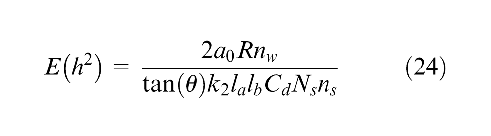
The square of the undeformed chip thickness, h², can be calculated by using the following equation

$$\begin{array}{cc}\multicolumn{1}{c}{E\left(h^2\right)}& =\underset{0}{\overset{\infty }{\int }}{h}^{2}f\left(h\right)\mathrm{dh}=\underset{0}{\overset{\infty }{\int }}\frac{h^3}{{\sigma }^2}{e}^{-\frac{h^2}{2{\sigma }^2}}\mathrm{dh}\hfill \\ \multicolumn{1}{c}{}& ={\left[e^{-\frac{h^2}{2{\sigma }^2}}(-2{\sigma }^2-h^2)\right]}_0^{\infty }=2{\sigma }^2\hfill \end{array}$$

(25)

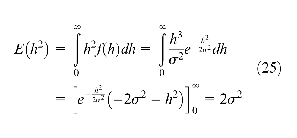
Rewriting equation (24) after substituting the expected values from equation (25) produces the equation

$$\sigma =\sqrt{\frac{a_{0}R{n}_w}{\tan \left(\theta \right)k_2{l}_a{l}_b{C}_d{N}_s{n}_s}}$$

(26)

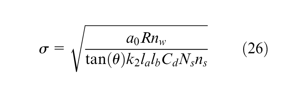
By substituting equation (26) into equation (16), the surface roughness can be expressed as

$$E\left(R_a\right)=0.463k_1\sqrt{\frac{a_{0}R{n}_w}{\tan \left(\theta \right)k_2{l}_a{l}_b{C}_d{N}_s{n}_s}}$$

(27)

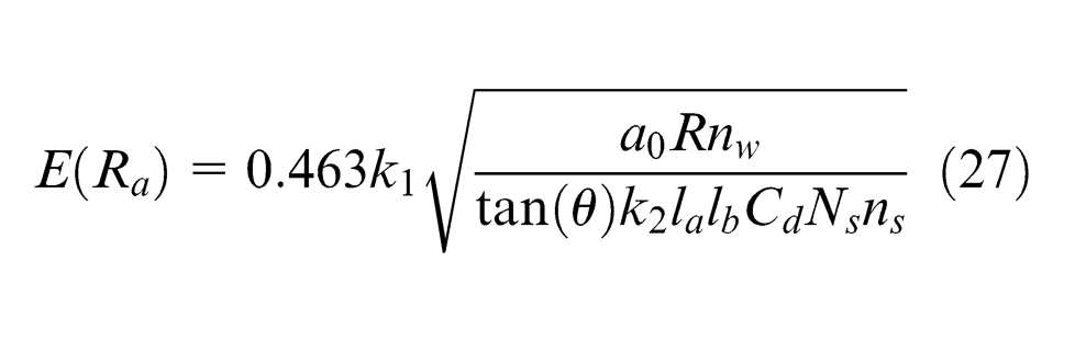
However, a dissimilarity between actual feed and theoretical feed occurs considering the elastic deformation of the grinding wheel and workpiece system. Therefore, a correction factor, k_s, is adapted to correct the theoretical roughness value derived from equation (27) and the final analytical expression is produced as follows

$$E\left(R_a\right)=0.463k_s{k}_1\sqrt{\frac{a_{0}R{n}_w}{\tan \left(\theta \right)k_2{l}_a{l}_b{C}_d{N}_s{n}_s}}$$

(28)

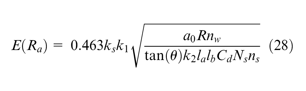
Equation (28) can be used to predict surface roughness based on the Rayleigh pdf of the abrasive grain protrusion heights.

Experimental setup and design

Experimental setup

The grinding experiments were conducted using a Model MD6050 CNC precision sphere grinding machine, the schematic of which is illustrated in Figure 1. The grinding wheel spindle power and the workpiece spindle power were 15 kW. The setup of the sphere grinding experiment is displayed in Figure 6(a). The matrix material of the workpiece sphere was 304 hardened steel. The coating material of the workpiece was WC-Co, the hardness of which was approximately 68 HRC, and the coating thickness was 0.4 mm. The sphere diameter, 2R, was approximately 234.2 mm and the sphere axial width, 2L, was approximately 175.6 mm. The vitreous bond grinding wheel was composed of an artificial diamond abrasive with 200 ANSI mesh size. The diamond wheel had a medium percentage of vitreous bond (L-grade hardness) and relatively high porosity to maintain the efficiency of self-sharpening. The size of the grinding cup wheel was approximately 176 mm in diameter and the wheel block size was 16 mm in length, 10 mm in width, and 10 mm in height. The cutting fluid used in all of the grinding tests was a semisynthetic water soluble Locks EP 204V cutting fluid.

Figure 6.

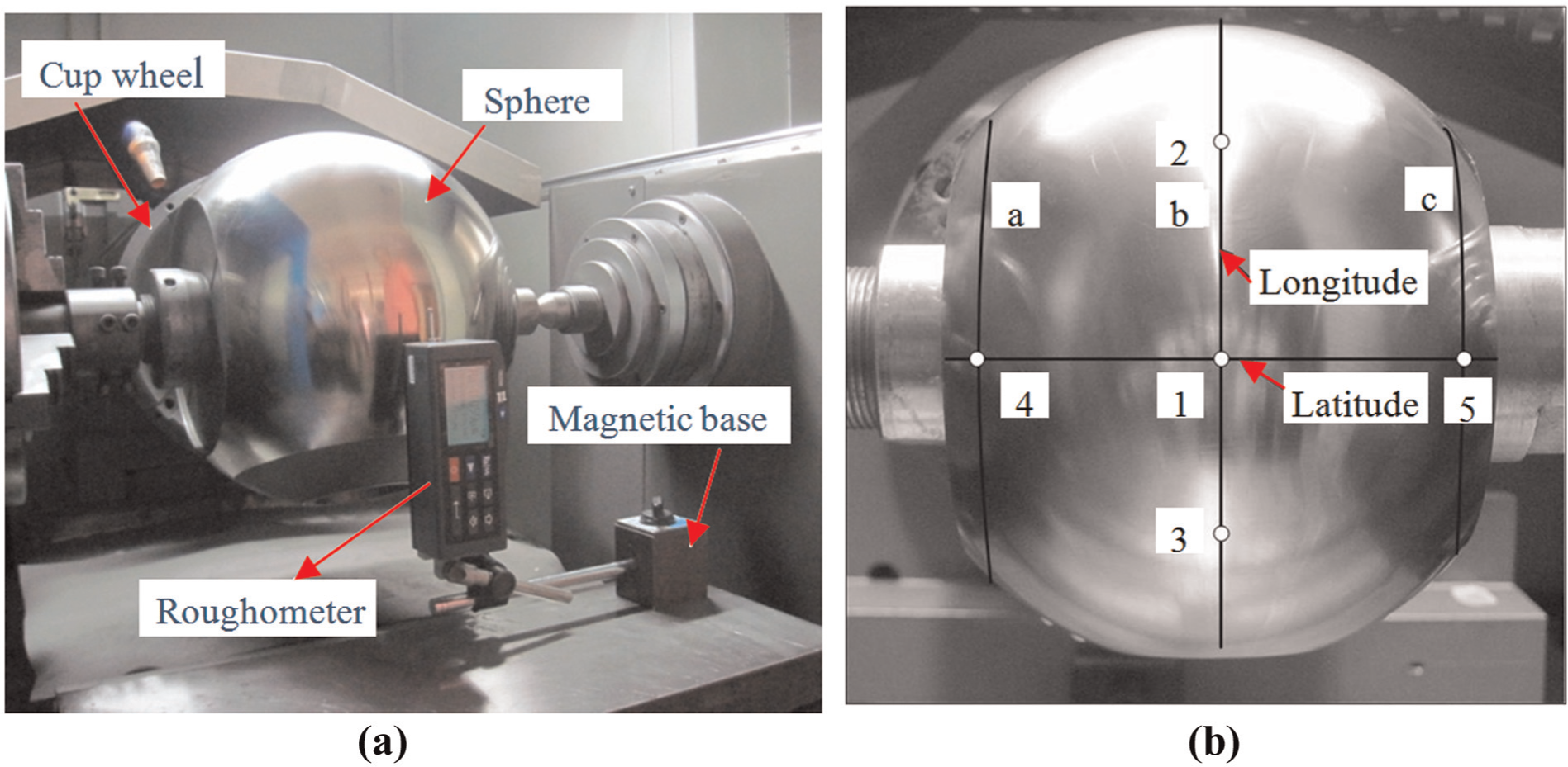
Spherical surface roughness measurement experiment: (a) experimental setup and (b) roughness measuring spots.

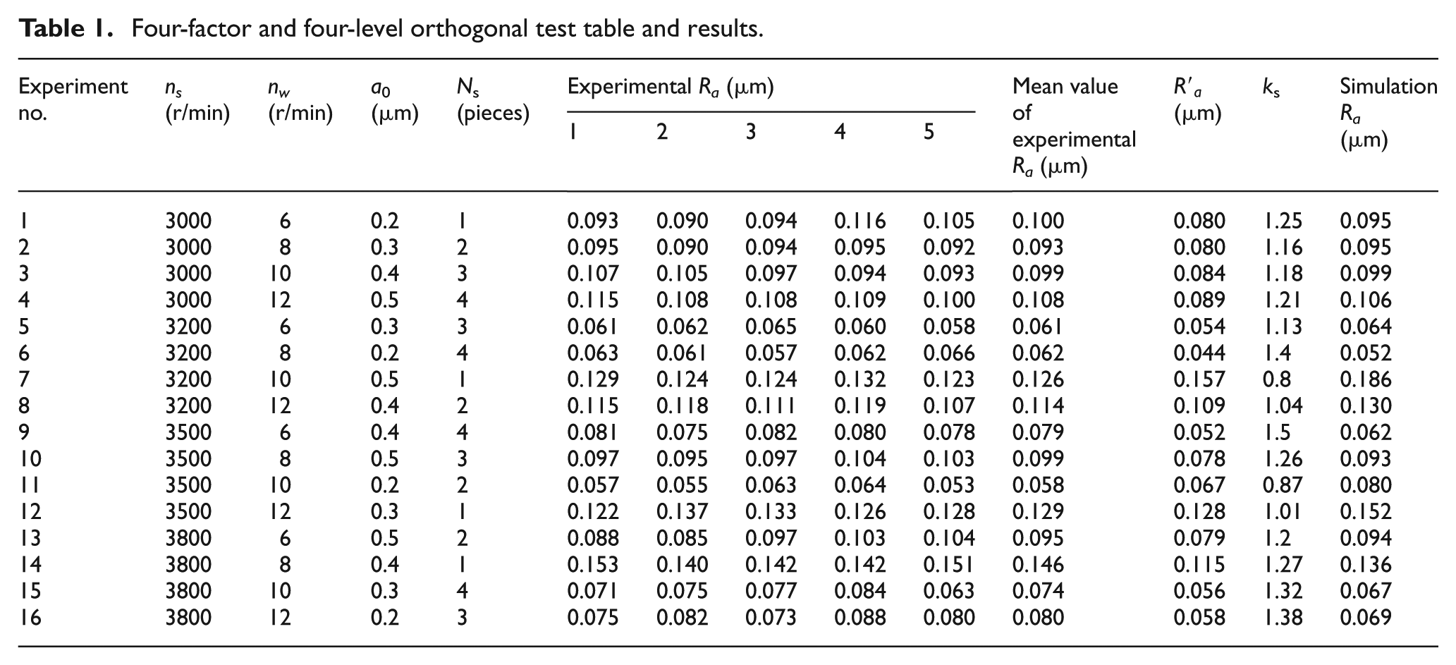
The diameter of the sphere was measured using an INSIZE model 3203-250AC outside diameter micrometer. The spherical surface roughness was measured using a Time Group TR200 surface roughometer. The roughness sensor TS110 was specifically designed for measuring curved surface roughness, and the measurement resolution was 0.01 µm. Roughness was measured at five points distributed evenly on the spherical surface, and the average value was the final result, which is displayed in Figure 6(b).

Experimental design

Experiments were designed to acquire the experimental spherical surface roughness values under various grinding conditions. These results were used to identify several parameters included in the presented roughness model, verify the theoretical roughness model, and study the effects of the grinding parameters on spherical surface roughness, which can be theoretically and experimentally analysed, and the result can verify the accuracy and robustness of the proposed roughness model.

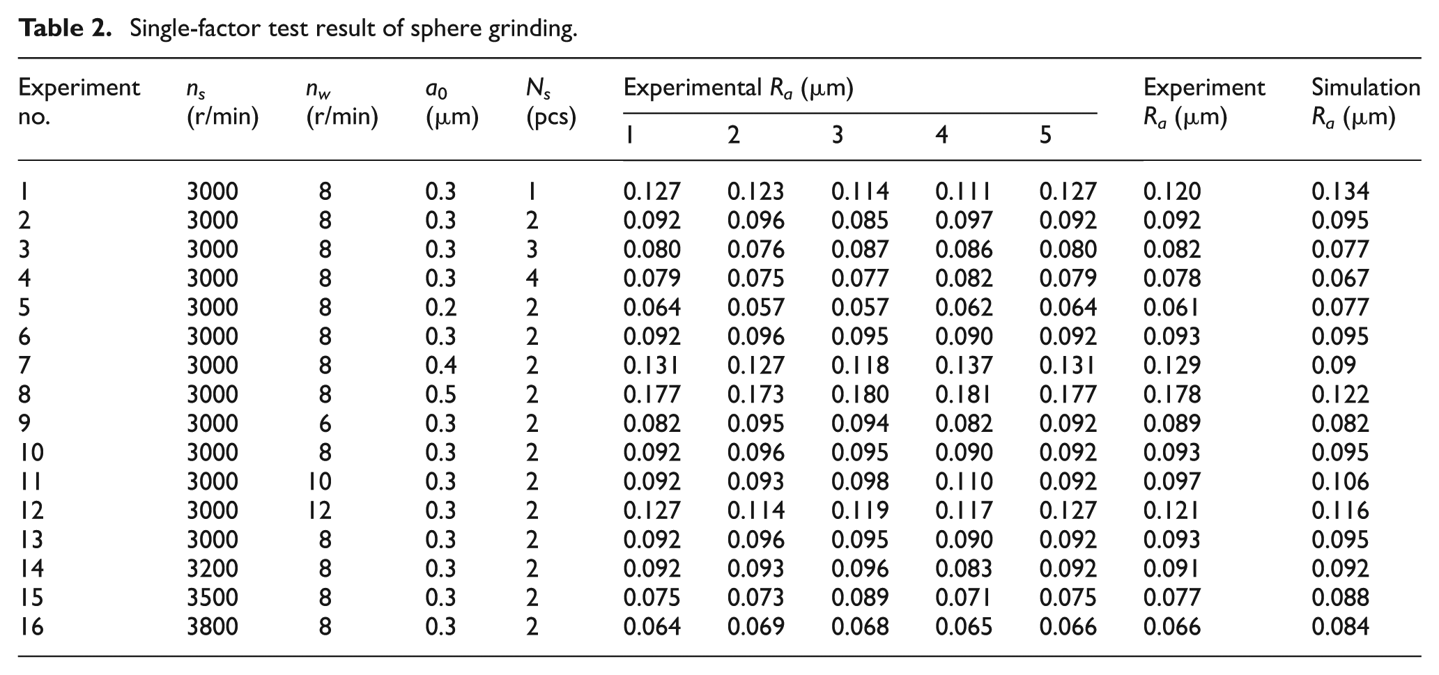
A four-factor and four-level orthogonal experiment table was designed to facilitate the identification of the k_s parameters, as displayed in Table 1. In this study, an orthogonal grinding test using four wheel speeds, n_s (3000, 3200, 3500, and 3800 r/min; that is, 37, 39, 43, and 47 m/s, respectively); four workpiece speeds, n_w (6, 8, 10, and 12 r/min); four feed rates, a₀ (0.2, 0.3, 0.4, and 0.5 µm/r); and four numbers of wheel blocks, N_s (1, 2, 3, and 4) was conducted to investigate spherical surface roughness. Sixteen tests were performed according to the orthogonal table, and the five surface roughness values were measured at five points distributed evenly on the spherical surface after each test.

Table 1.

Four-factor and four-level orthogonal test table and results.

Experiment no.	ns (r/min)	nw (r/min)	a 0(µm)	N s (pieces)	Experimental Ra (μm)					Mean value of experimental Ra (µm)	${R\prime }_a$ (µm)	k s	Simulation Ra (µm)
					1	2	3	4	5
1	3000	6	0.2	1	0.093	0.090	0.094	0.116	0.105	0.100	0.080	1.25	0.095
2	3000	8	0.3	2	0.095	0.090	0.094	0.095	0.092	0.093	0.080	1.16	0.095
3	3000	10	0.4	3	0.107	0.105	0.097	0.094	0.093	0.099	0.084	1.18	0.099
4	3000	12	0.5	4	0.115	0.108	0.108	0.109	0.100	0.108	0.089	1.21	0.106
5	3200	6	0.3	3	0.061	0.062	0.065	0.060	0.058	0.061	0.054	1.13	0.064
6	3200	8	0.2	4	0.063	0.061	0.057	0.062	0.066	0.062	0.044	1.4	0.052
7	3200	10	0.5	1	0.129	0.124	0.124	0.132	0.123	0.126	0.157	0.8	0.186
8	3200	12	0.4	2	0.115	0.118	0.111	0.119	0.107	0.114	0.109	1.04	0.130
9	3500	6	0.4	4	0.081	0.075	0.082	0.080	0.078	0.079	0.052	1.5	0.062
10	3500	8	0.5	3	0.097	0.095	0.097	0.104	0.103	0.099	0.078	1.26	0.093
11	3500	10	0.2	2	0.057	0.055	0.063	0.064	0.053	0.058	0.067	0.87	0.080
12	3500	12	0.3	1	0.122	0.137	0.133	0.126	0.128	0.129	0.128	1.01	0.152
13	3800	6	0.5	2	0.088	0.085	0.097	0.103	0.104	0.095	0.079	1.2	0.094
14	3800	8	0.4	1	0.153	0.140	0.142	0.142	0.151	0.146	0.115	1.27	0.136
15	3800	10	0.3	4	0.071	0.075	0.077	0.084	0.063	0.074	0.056	1.32	0.067
16	3800	12	0.2	3	0.075	0.082	0.073	0.088	0.080	0.080	0.058	1.38	0.069

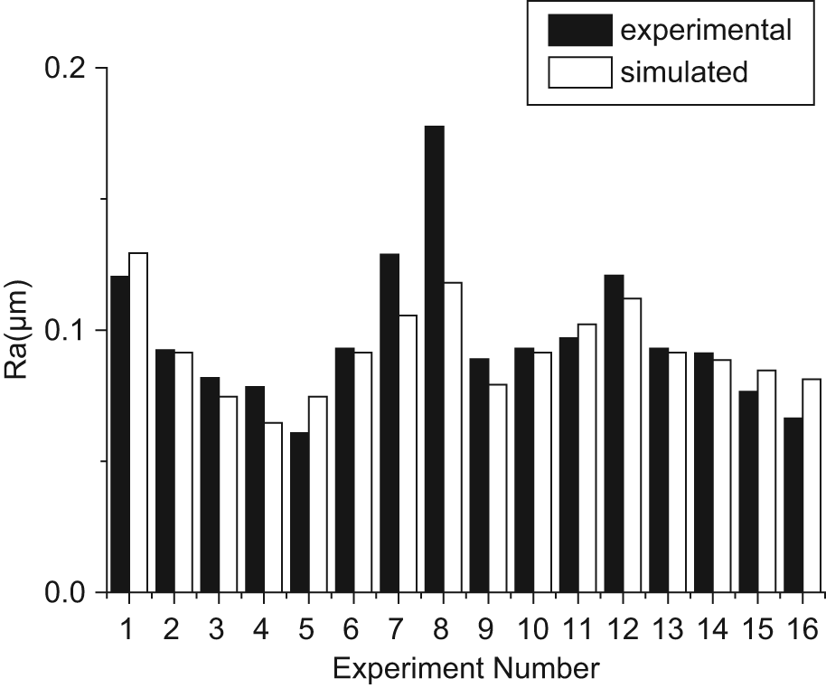
To study the effect of grinding parameters on surface roughness, four single-factor tests were designed. The single factors were wheel speed, workpiece speed, feed rate, and the wheel number. Each factor contained four levels, which are illustrated in Table 2. Other grinding conditions involved in the single-factor tests, and the roughness measurement method were the same as those used in the orthogonal test.

Table 2.

Single-factor test result of sphere grinding.

Experiment no.	ns (r/min)	nw (r/min)	a 0 (μm)	Ns (pcs)	Experimental Ra (μm)					Experiment Ra (μm)	Simulation Ra (μm)
					1	2	3	4	5
1	3000	8	0.3	1	0.127	0.123	0.114	0.111	0.127	0.120	0.134
2	3000	8	0.3	2	0.092	0.096	0.085	0.097	0.092	0.092	0.095
3	3000	8	0.3	3	0.080	0.076	0.087	0.086	0.080	0.082	0.077
4	3000	8	0.3	4	0.079	0.075	0.077	0.082	0.079	0.078	0.067
5	3000	8	0.2	2	0.064	0.057	0.057	0.062	0.064	0.061	0.077
6	3000	8	0.3	2	0.092	0.096	0.095	0.090	0.092	0.093	0.095
7	3000	8	0.4	2	0.131	0.127	0.118	0.137	0.131	0.129	0.09
8	3000	8	0.5	2	0.177	0.173	0.180	0.181	0.177	0.178	0.122
9	3000	6	0.3	2	0.082	0.095	0.094	0.082	0.092	0.089	0.082
10	3000	8	0.3	2	0.092	0.096	0.095	0.090	0.092	0.093	0.095
11	3000	10	0.3	2	0.092	0.093	0.098	0.110	0.092	0.097	0.106
12	3000	12	0.3	2	0.127	0.114	0.119	0.117	0.127	0.121	0.116
13	3000	8	0.3	2	0.092	0.096	0.095	0.090	0.092	0.093	0.095
14	3200	8	0.3	2	0.092	0.093	0.096	0.083	0.092	0.091	0.092
15	3500	8	0.3	2	0.075	0.073	0.089	0.071	0.075	0.077	0.088
16	3800	8	0.3	2	0.064	0.069	0.068	0.065	0.066	0.066	0.084

Identification of model parameters

Internal cone angle, 2θ

According to statistical laws, the internal cone angle, 2θ, ranges between 80° and 145°. Studies have indicated that the proportion of 2θ is associated with grain size, and 2θ slightly increases as the grain width increases. ¹³ A diamond-particle ceramic matrix grinding wheel was used in the experiments and an average (among all of the grains recorded) cone angle of 2.5 radians (143°) was obtained, which represents an attack angle of approximately 18°. ¹⁴

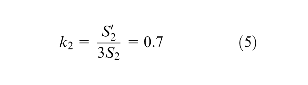
Overlap factors, k₁ and k₂

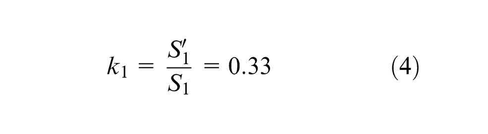
Although optimal methods for measuring the overlap factors k₁ and k₂ have not been developed, the values can be determined by using theoretical analysis. According to equations (4) and (5), k₁ = 0.33 and k₂ = 0.7.

Dynamic cutting edge density, C_d

Dynamic cutting edge density, C_d, is the number of active grits per unit area and can be obtained using a microscope measurement method. In the experiments, a three-dimensional digital measuring instrument, the Keyence VH-8000, was used to observe the number of grains on the grinding wheel surface at 175× magnification. The average number of active grits per unit area was C_d = 3 (mm⁻²).

Correction factor, k_s

Roughness experiments regarding sphere grinding were used to identify and validate the value of the correction factor, k_s, because k_s cannot be obtained by using theoretical analysis or mathematical derivation. Changing variables, such as the material of the workpiece or abrasive, require a new calibration to refresh k_s.

Results and discussion

Results

The results of the four-factor and four-level orthogonal experiment are displayed in Table 1. The five spherical roughness values were recorded, and the arithmetic mean of these values was calculated.

As illustrated in Table 1, ${R\prime }_a$ is the uncorrected simulation roughness. The average of the correction factor is expressed as k_s = Σk_si/16 = 1.19. Thus, the expected value of corrected-simulation surface roughness can be calculated by using equation (28), and the R_a results are displayed in Table 1.

The results of the single-factor test are displayed in Table 2. Each factor consisted of four levels. The grinding parameters are listed in Table 2. The experimental spherical roughness results were recorded, and the arithmetic mean of the values was calculated. The theoretical simulation roughness value, R_a, was also calculated based on the roughness model, and is listed in Table 2.

Comparison between the results of experiment and simulation

Figure 7 is a bar chart that displays the experimental values and simulation values of the ground spherical surface roughness derived from the single-factor test. The value of the correction factor, k_s, was the same as the value calculated in the orthogonal experiment. Figure 7 reveals that the experimental values and simulation values of R_a exhibit the same trend. Although a low number of results produce a large deviation, the simulation values were reasonably similar to the experimental results. This indicates that the surface roughness model is effective and robust considering the changes in the values of process parameters. To validate this surface roughness model further, the absolute value of the relative error between the experimental values and simulation values was calculated. As displayed in Figure 8, the maximum error was 33.5%, and the average error was approximately 10.4%. This is considered a favourable prediction of ground spherical surface roughness.

Figure 7.

Experimental and simulated spherical surface roughnesses.

Figure 8.

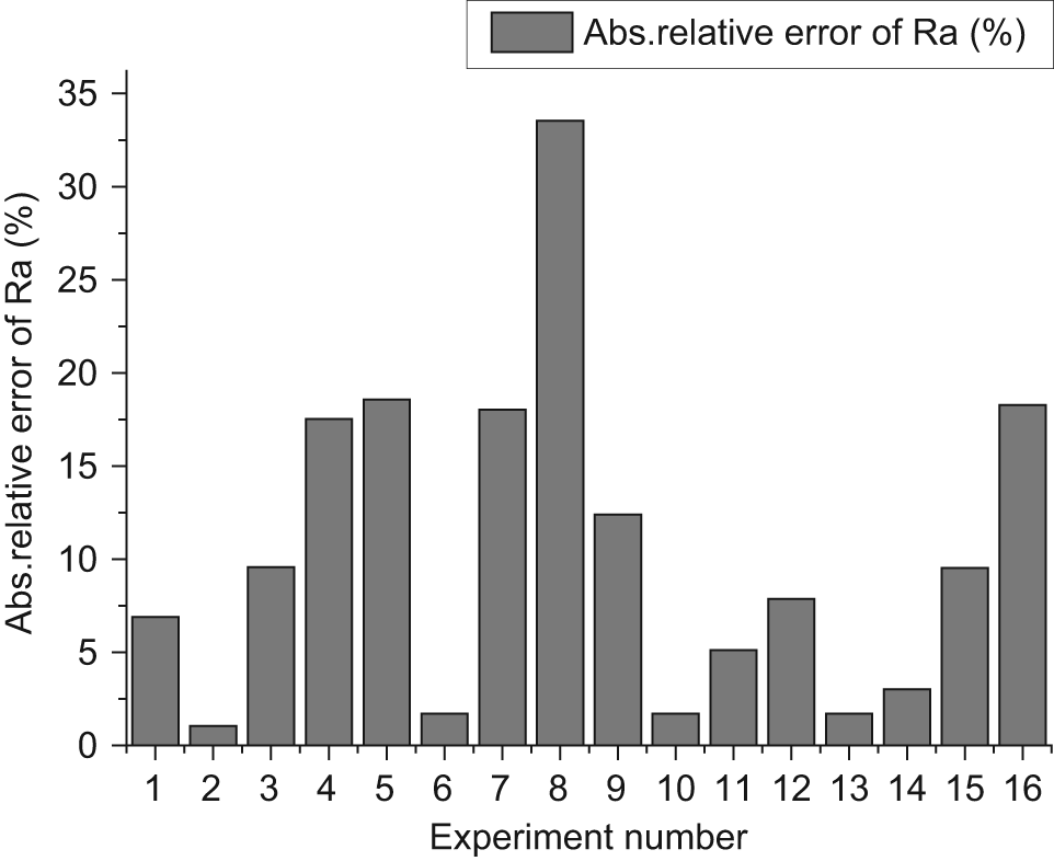
Absolute relative error between the measured and the predicted R_a values.

The effect of grinding parameters on surface roughness

The influence of feed on surface roughness

The change in surface roughness is illustrated in Figure 9. The feed rate, a₀, increased from 0.2 µm/r to 0.5 µm/r when the wheel speed, n_s, was 3000 r/min; the workpiece speed, n_w, was 8 r/min; and the number of wheels, N_s, was two. As indicated in Figure 9, as the feed rate increased, the trend of roughness increased. The roughness increased because the increasing feed rate caused the undeformed chip thickness to increase.

Figure 9.

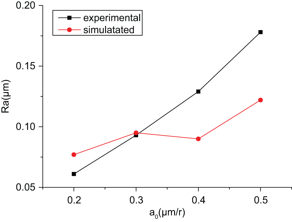
Spherical surface roughness presented at various values of feed rate.

The influence of workpiece speed on surface roughness

The change in surface roughness is illustrated in Figure 10. The workpiece speed, n_w, increased from 6 to 12 r/min when the wheel speed, n_s, was 3000 r/min; the feed rate, a₀, was 0.3 µm/r; and the number of wheels, N_s, was two. As indicated in Figure 10, as the workpiece speed increased, the trend of roughness was increasing as a whole. This trend can be explained based on the roughness model, which indicates that the increasing workpiece speed caused the distance between grooves on the surface to increase.

Figure 10.

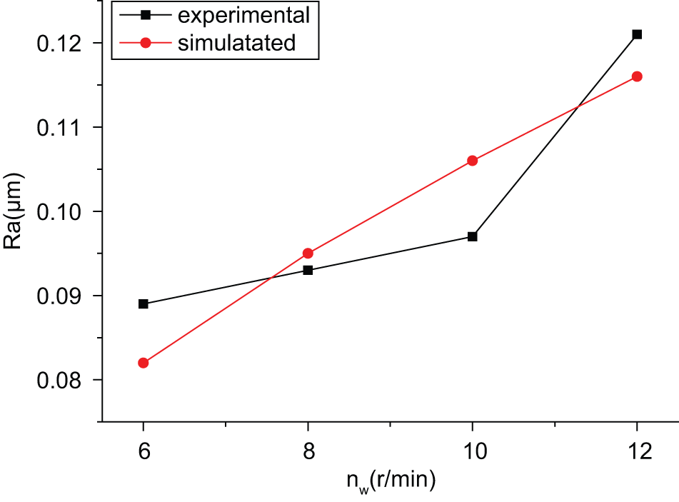
Spherical surface roughness presented at various values of workpiece speed.

The influence of wheel speed on surface roughness

The change of surface roughness is illustrated in Figure 8. The wheel speed, n_s, increased from 3000 to 3800 r/min when the workpiece speed, n_w, was 8 r/min; the feed rate, a₀, was 0.3 µm/r; and the number of wheels, N_s, was two. As indicated in Figure 11, as the wheel speed increased, the trend of roughness was decreasing as a whole. This phenomenon can be explained based on the proposed roughness model, which indicates that the track density on the surface increased as the wheel speed increased.

Figure 11.

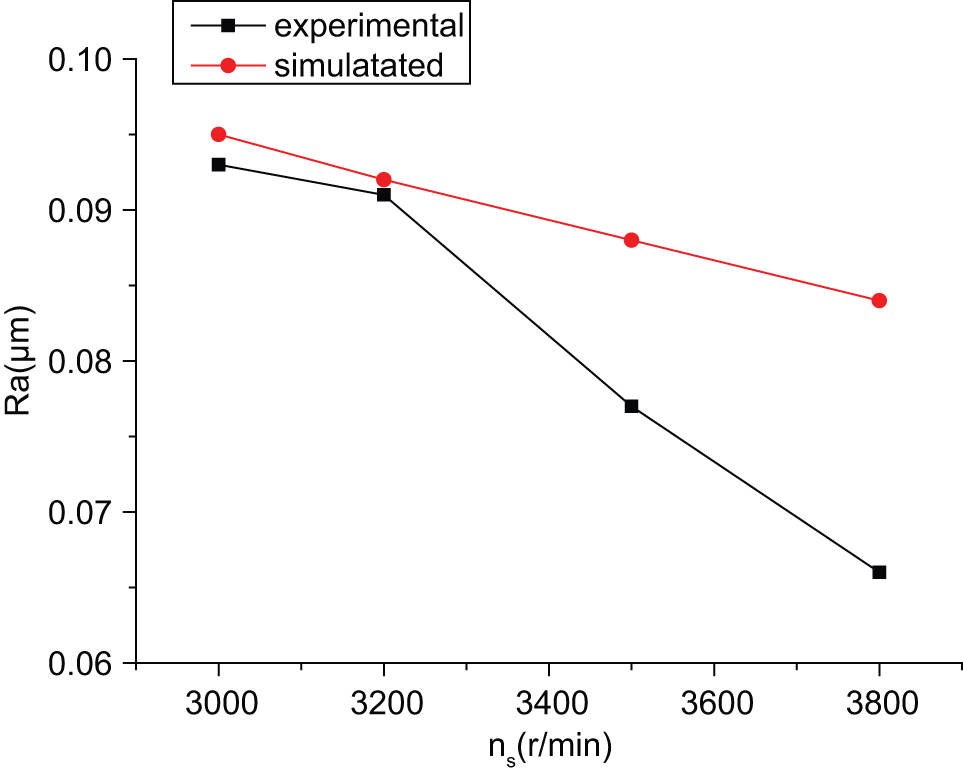
Surface roughness presented at various values of wheel speed.

The influence of wheel number on surface roughness

The change of surface roughness is illustrated in Figure 12. The wheel number, N_s, increased from one piece to four pieces when the workpiece speed, n_w, was 8 r/min; the feed rate, a₀, was 0.3 µm/r; and the wheel speed, n_s, was 3000 r/min. As indicated in Figure 12, as the wheel number increased, the trend of roughness was decreasing in general. This occurred because as the wheel number increases, the track density on the surface increases, and undeformed chip thickness decreases.

Figure 12.

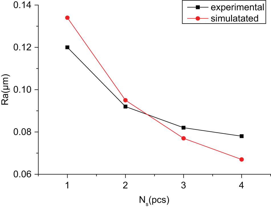
Surface roughness presented at various values of wheel number.

According to this analysis, the ground spherical surface roughness is affected by numerous grinding parameters. Based on the analysis of the roughness model, the effects of the four primary factors on the spherical surface roughness were studied. The results of both the experiment and simulation indicate that as the feed rate and workpiece speed increased, the surface roughness increased in general, and that as the wheel speed and wheel number increased, the surface roughness decreased in general. This analysis also demonstrates that the theoretical roughness values are reasonably similar to those of the experimental results. However, when choosing the proper values of parameters for favourable surface roughness, other factors such as grinding efficiency and grinding forces must be considered. For example, increasing the wheel number causes the grinding force to increase, thus allowing the other conditions to remain unchanged, and the feed rate must be sufficiently small, which will inversely influence the grinding efficiency.

Conclusion

In this article, an analytical model for predicting spherical surface roughness in spherical grinding is presented for the first time. The model is based on the undeformed chip thickness model and the Rayleigh pdf of the abrasive grain protrusion heights and incorporates the overlapping effect of grooves generated by the grains that interact with the workpiece. Experiments were designed to acquire the experimental spherical surface roughness values under various grinding conditions, and the method for identifying several parameters of the presented roughness model is introduced. The predicted surface roughness is consistent with that derived from the experimental data obtained under various grinding conditions. Furthermore, the effects of the grinding parameters, including the wheel feed, wheel speed, workpiece speed, and the number of wheel blocks, on spherical surface roughness were theoretically and experimentally studied. The results reveal the influence of these process parameters, which assists in optimising parameter selection, and further verifies the proposed roughness model.