
Abstract
The duopoly model with a Cournot form under random yield has received little attention. This article revisits the classic Cournot duopoly competition model by considering manufacturer yield uncertainty. We analyze the model under symmetric, asymmetric and monopoly situations. The manufacturers’ best production policy and expected market share are compared with each other in each situation. The expected market outputs of the three models are also compared under certain conditions. In the asymmetric case, the asymmetric model is extended by considering a powerful oligarch who can exert influence on her rival’s production decision by releasing her cost-type information. We derive that the maximization of the stronger manufacturer’s expected profit is highly correlated with consumer surplus. Numerical examples are presented to illustrate the results.
Introduction
Research on static and dynamic oligopolies is one of the richest areas in the economics literature. Since the by now famous duopoly theory was first explained by Cournot in 1838, many scholars have examined oligopoly models and their extensions. A comprehensive review of results about the single-product model was provided by Okuguchi, 1 and the extensions of multiple products extensions with applications were discussed by Okuguchi and Szldarovszky. 2 Long and Soubeyran 3 provided a new proof of the existence and uniqueness of a Cournot equilibrium characterized in terms of marginal costs. Most of the models discussed in the literature have assumed that the firms have full knowledge of all price functions as well as are able to respond instantly to the rival firm’s outputs and price decisions. However, there is a basic underlying presumption that the quantity a firm intends to produce equals the final output production quantity. In fact, almost every manufacturing firm suffers from yield uncertainty, namely, that the final output does not always equal the firm’s target production quantities. Thus, it would be worthwhile to reconsider the classic Cournot competition model under yield randomness.
In many industries, the final output quantity of a production process is not deterministic and is influenced by many factors. For example, weather is one of the most important factors that affect agriculture-related industries; yet, when planting decisions are made, it is almost impossible to precisely forecast the weather in the future. Chiu et al. 4 considered the algebraic derivation for the production lot-sizing problem with backlogging, random defective rate and rework. They extend the classic economic production quantity (EPQ) model to a modified model by taking backlogging, random defective rate and rework into consideration. Hsu and Hsu 5 developed an integrated inventory model for the coordination of a two-echelon supply chain under an imperfect vendor production process. They assume that the proportion of defective items in each production lot is stochastic and follows a known probability density function. Dada et al. 6 considered the procurement problem of a newsvendor that is served by multiple suppliers, where the supplier is defined to be either perfectly reliable or unreliable. There have been some attempts at modeling the production and procurement decisions in supply chain management involving risk supply. Xu 7 tried to manage production and procurement in a decentralized supply chain with random supplier yield and stochastic manufacturer demand through option contracts. Babich et al. 8 studied the effects of disruption risk in a supply chain where one retailer deals with competing risky suppliers who may default during their production lead times. The phenomenon of yield uncertainty can also be found in remanufacturing companies. Bakal and Akcali 9 investigated the pricing decisions in a remanufacturing supply chain with random recovery yield rate. Mukhopadhyay and Ma 10 studied the production and procurement problem of an integrated manufacturing and remanufacturing system by considering yield randomness in recycling.
The studies above mainly discuss the ordering and production policies in a single supplier–vendor supply chain. Vendor with multiple suppliers should also be of concern. Deo and Corbett 11 formulated a two-stage model of Cournot competition with N-symmetric firms and analyzed the effect of yield uncertainty on firms’ entry and production decisions. Tang and Kouvelis 12 presented supplier diversification strategies by considering yield uncertainty and buyer competition, but the production decision strategies between competing suppliers with random yield in a market when there is no retailer has been insufficiently studied. Xanthopoulos et al. 13 proposed a single-period inventory model for capturing the trade-off between inventory policies and disruption risks in a dual-sourcing supply chain. Yan et al. 14 studied supplier diversification in a multiple supplier competition model with random yield under symmetric environment by considering a case in which the suppliers’ random yields are correlated. Yu et al. 15 focused on evaluating the impacts of supply disruption risks on the choice between single- and dual-sourcing methods in a two-stage supply chain with nonstationary and price-sensitive demand. The above work mainly focused on the ordering policy of the vendor from a supply chain perspective while neglecting the production strategies of the manufacturers.
However, competition among manufacturers does change the structure of the market. Deo and Corbett 11 and Yan et al. 14 studied the random yield problem in a market with manufacturers who have symmetric information and the same costs. Therefore, it is worthwhile to study how manufacturers with different costs compete under asymmetric or monopoly situations. The duopoly model with a Cournot form under random yield has received little attention. Yet, few researchers have worked on this problem with yield randomness. The motivation for exploring the topic is to try to answer the following questions: (1) How do duopoly manufacturers compete or cooperate under random yield in a noncooperative or monopoly situation? (2) What is the impact of yield uncertainty on the duopoly manufacturers’ production policy and the market output? and (3) Which manufacturer shares a larger market share under random yield?
In this article, we remodel the classic Cournot production competition model by using the stochastic proportional yield model under noncooperative (symmetric and asymmetric) and monopoly conditions, respectively, to try to derive the best target production quantities for the duopoly manufacturers. Then, our model is extended by considering a powerful oligarch who can exert influence on her rival’s production decision not only by her own production decision but also by releasing her cost-type information.
The objective of this article is to reconsider the classic Cournot duopoly competition model under yield uncertainty. We aim to derive the equilibrium target production policies for the duopoly and analyze the impact of production yield uncertainty on the equilibrium outcome and the social optimum for the classic Cournot model of duopoly competition and monopoly under yield uncertainty. The results of this article can be applied in particular to Cournot-characteristic industries, which are industries that supply necessities of life: oil, plant production, tap water and electricity, for instance. Likely users of this research are manufacturers in these industries, who can use the model in setting their best target production quantities under yield uncertainty.
The rest of this article is organized as follows: In section “Model formulation,” we present the basic model and related literatures. Sections “Symmetric Cournot duopoly with random yield” and “Asymmetric Cournot duopoly with random yield” study the Cournot competition model under random yield and outline the competitive equilibrium under a symmetric and asymmetric environment, respectively. Section “The case of Cartel-monopoly” focuses on the situation in which the duopolists cooperate to monopolize the market in order to reach maximum revenue. Section “An extension: ρ is ‘made’ and released by M2” extends the asymmetric model to consider a stronger oligarch who can exert influence on her rival’s production decision by releasing her cost-type information. Numerical examples are presented to illustrate the results and study the effect of yield uncertainty on the market.
Model formulation
Consider a single-period model in a local market consisting of two manufacturers denoted by Mi (i = 1,2). The duopoly manufacturers make the same final products and compete in their production quantities at the same time. Their aims are to decide their best target production quantities to maximize their profit. Mi competes in output Qi (i = 1,2). qi (i = 1,2) denotes their planed production quantities and equals their final production quantity when there is no production risk. However, by considering random yields, their actual realized production quantities are Qi = αiqi, where αi (i = 1,2) is a random variable attached to the planned production quantity qi representing the yield risk of manufacturer i. Because it is impossible to avoid yield uncertainty, the two manufacturers can only decide their target production quantities to maximize their expected profit. Yano and Lee 16 presented a thorough review of single-stage single-period models that dealt with lot-sizing models with stochastically proportional yield models, especially when the yield losses in the production process and the final production quantities are not predictable in manufacturing systems. Furthermore, we assume that αi is independent but with an identical probability distribution. For example, there are two farms in the same area planting the same crop with the same seed and planting techniques. They suffer the same yield risk, which is mainly determined by the weather, and their production processes are independent. Thus, it is feasible to assume “α” as an independent and identically distributed variable. The mean and variance of αi are denoted by µ = E(αi) and σ 2 = Var(αi) (0 < µ < 1, σ > 0), respectively. This form of random yield has been used by many researchers, such as Yan et al., 14 Agrawal and Nahmias, 17 Li and Zheng 18 and Keren. 19 Note that, as a special case, our formulation covers the model in the studies by Creane 20 and Serel, 21 where the yield risk αi is a Bernoulli distributed variable. We assume that the manufacturers’ final production quantities are realized with a nonzero probability.
The manufacturers’ retail price (market price) of the product is given by the linear reverse demand curve p = k−bQt (k, b > 0), where k is the reservation price, b is the elasticity coefficient and Qt stands for the total output of M1 and M2. There are two marginal costs for the manufacturers: one is the unit-preparing production cost ci1 and the other is the unit-realized production quantity cost ci2. This type of production cost has been used by many researchers, such as Deo and Corbett
11
and Kazaz.
22
Then the manufacturer’s sales revenue is
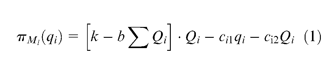
Without taking into consideration of random yield (Qi = qi), the solution of equation (1) will be the classical Cournot production competition model. However, because of disruptions such as human error, technical error, weather and so on, yield uncertainty exists almost in every production system, especially in agriculture production. Thus, the final output or profit cannot be effectively predicted, and the only thing they can do is to choose a best target production quantity to maximize their expected profit when αi is stochastically distributed. Section “Symmetric Cournot duopoly with random yield” will focus on the manufacturers’ optimal decisions under symmetric condition with random yield.
Symmetric Cournot duopoly with random yield
This section examines the scenario in which two manufacturers compete with full information about their mutual costs. Each manufacturer sets her target production quantity qi, and after realizing the production risk αi, we have the total production quantity as
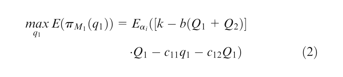
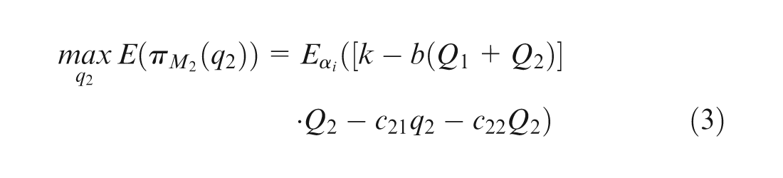
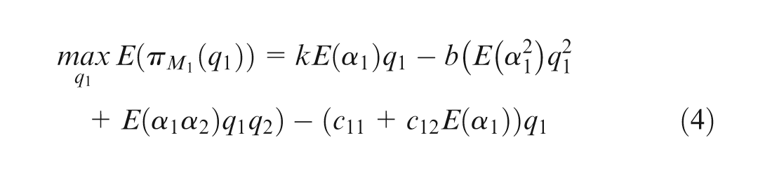
By substituting Qt = α1q1+α2q2 into the above two equations, equations (2) and (3) can be rewritten as

Because M1 and M2 decide their target production quantities at the same time, the Nash equilibrium production quantity
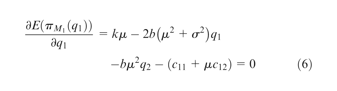
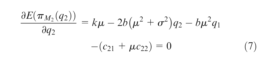
Let

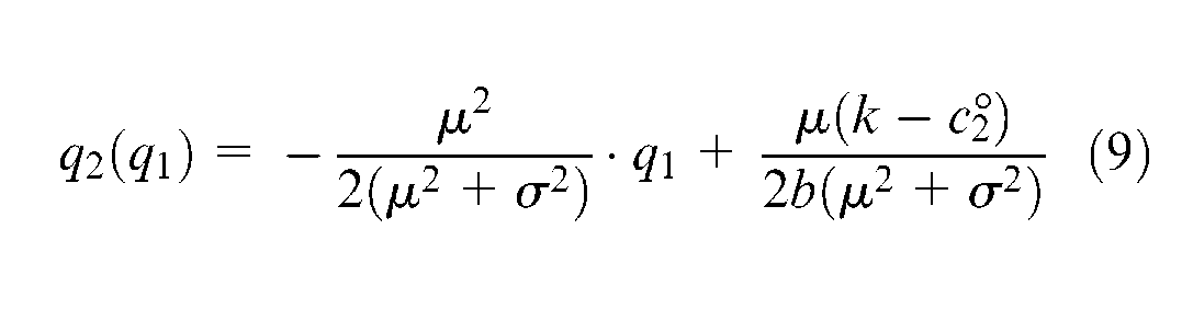
Equations (8) and (9), respectively, denote the production policy reaction function for the duopoly manufacturers under random yield. To ensure that
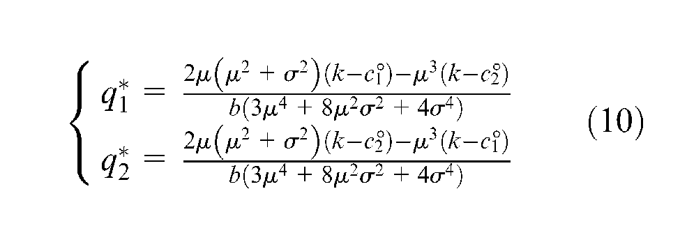
Theorem 1. Under random yield, there exists a unique Nash best target production quantity equilibrium for the duopoly manufacturers in a single-period symmetric environment
Proposition 1. In the symmetric case, a manufacturer with lower cost has a larger (expected) market share, that is, (i) if
Proof.
Lemma 1. In the symmetric case, the expected market output decreases with respect to δ.
Proof.
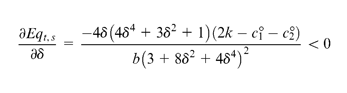
The introduction of the δ facilitates the analysis of the effect of yield randomness on the expected market output. Lemma 1 indicates that, if µ is fixed, Eqt,s decreases in σ. Furthermore, if we fix µ = 1, σ = 0 (δ = 0, the deterministic yield condition), as Eqt,s is decreasing in δ, then Eqt,s < qt,s (δ = 0). Thus, the expected market output under yield uncertainty is smaller compared with the deterministic yield condition. From equation (10), we can also derive
Figure 1 illustrates the effect of random yield on the production reaction function of the duopoly manufacturers. Solid lines l1 and l2, respectively, denote M1 and M2’s production reaction curve under deterministic yield. The curve can be obtained by setting µ = 1, σ = 0 in equations (8) and (9). The shadow between the parallel dash lines, lying on both sides of the solid line, stands for the fluctuation effect on M1’s target production reaction under random yield.
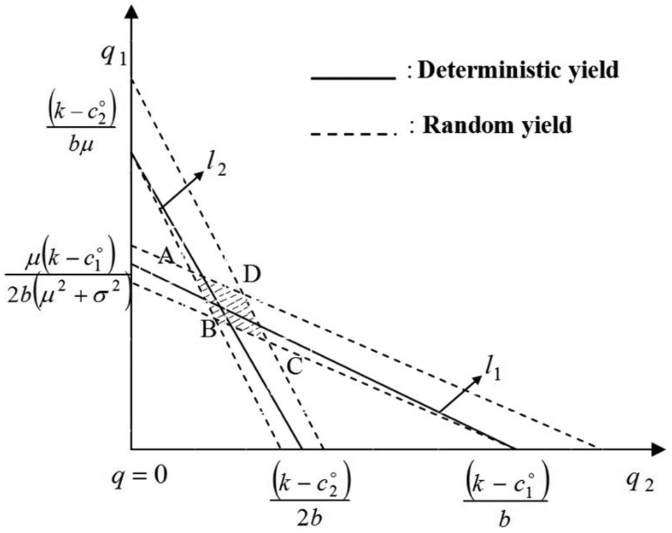
The impact of random yield on the production reaction of the duopoly.
The slope coefficient of the reaction curve of M1 under yield uncertainty can be derived from equations (8) and (9).
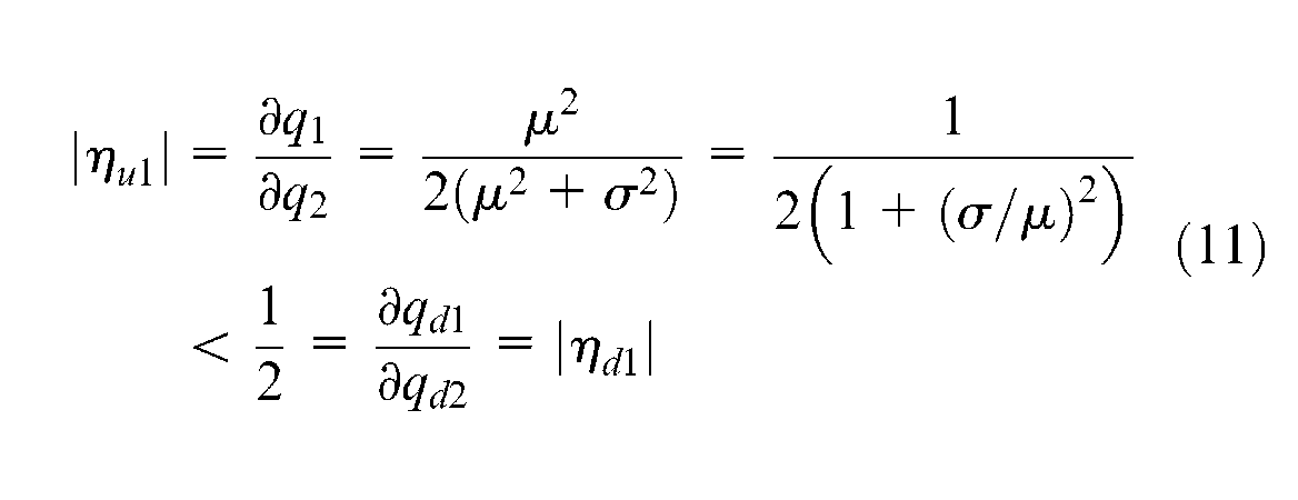
It can be observed in Figure 1 that the slope coefficient of the reaction curve of M1 under yield uncertainty is smaller than that of the corresponding solid line, which also exists for M2. An explanation for equation (11) could be that yield uncertainty decreases the reaction on their mutual target production quantity. The actual location of the reaction curve under random yield (dash line) depends on the comparison of
Asymmetric Cournot duopoly with random yield
Information asymmetry exists widely in competitive markets, especially in oligopoly competition. Vives
23
analyzed an incomplete information setting where firms receive signals about uncertain demand, and they proved that the Bertrand Bayesian–Nash quantity is higher than the Cournot Bayesian–Nash quantity. Lofaro
24
studied the efficiency of Cournot and Bertrand competition under incomplete information environment. However, their results would be changed if yield uncertainty was considered. In this section, a Cournot duopoly production competition model with incomplete cost information under random yield is analyzed. Here, we assume that M1 produces at a constant unit production cost
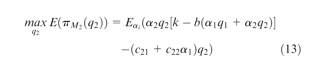
Assuming that M2 has accurate knowledge about M1’s cost, M2 should make her production decision (q2) to maximize her profit function as
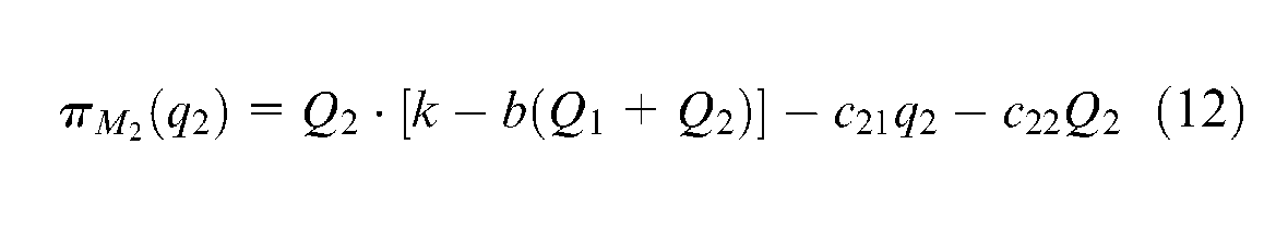
By considering the random yield risk αi, M2 will choose the best target production quantity
By using a similar transformation as in section “Symmetric Cournot duopoly with random yield,” here we set
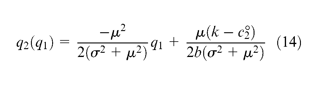
Equation (14) explains that M2’s best production target quantity depends not only on the target production quantity of M1 but also depends on her own unit production cost. To set,
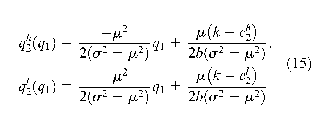
By observing the equations above, it is easy to find that 2b(σ
2
+µ
2
), the denominator of q2, is a positive constant. To ensure q2 is positive, the numerator must also be positive, such that
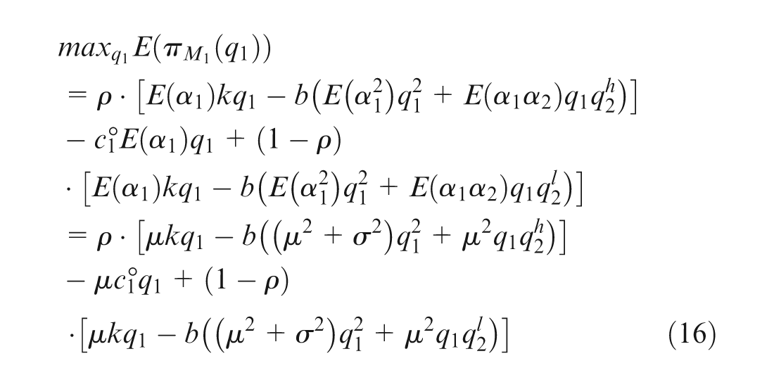
To solve the first-order condition of equation (16) with respect to q1, the reactive production function of M1 upon M2 should satisfy
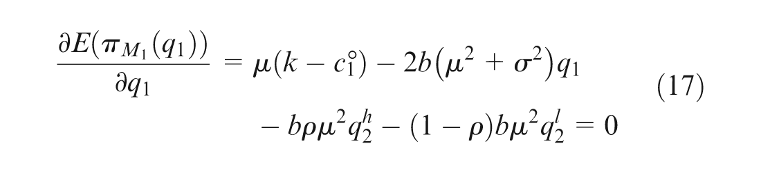
Because M1 is not sure about M2’s cost type, it is hard to get the exact reaction curve of M1 as in Figure 1. By substituting equation (15) into equation (17), and using simple algebraic manipulation, we have Theorem 2:
Theorem 2. Under random yield, there exists a unique Bayes–Nash equilibrium best target production quantity for the duopoly manufacturers in a single-period asymmetric environment
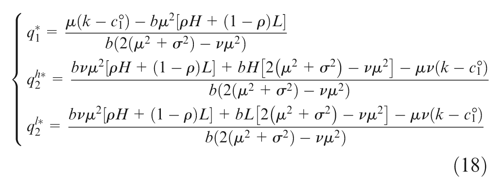
where
Lemma 2. M2’s best target production quantity
Proof. To derive the first-order condition of
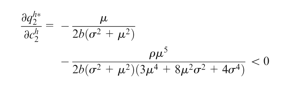
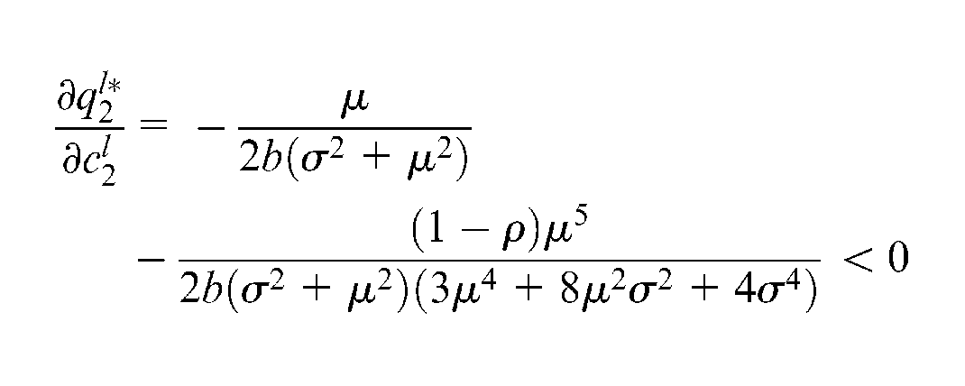
Thus, M2’s best production quantity q2 decreases with her cost
Lemma 3. (i) M1’s best target production quantity
Proof of (i). Derive the first-order condition of
Proof of (ii). From equation (18), we have
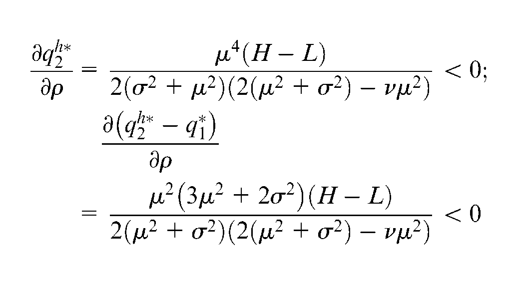
The case of the low cost–type M2 can also be proved. Recall that M1’s best target production quantity q1 is proportional to ρ and M2’s best target production quantity q2 decreases when ρ increases. Hence, the difference of q2 and q1 decreases with the increase of ρ.
Lemma 4. (i) The expected market output in the asymmetric case increases with the probability ρ that M1 believes M2 is high cost type and (ii) the expected market output is larger than the symmetric case when M2 is low cost type and is smaller when M2 is high cost type.
Proof of (i). Take high cost–type M2, for example,
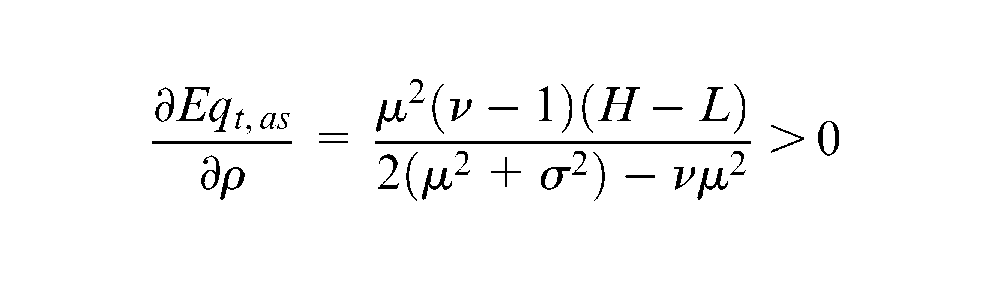
which proves (i).
Proof of (ii). This is obtained by solving the difference of
To derive the first-order condition of the difference with respect to ρ, we have
When M2 is high cost type, if ρ = 1, we have
(i) indicates that information asymmetry has a positive effect in enlarging the market scale. (ii) shows that whether information asymmetry magnifies the expected market output compared with the symmetric case depends on M2’s cost type. By observing equations (10) and (18), it is interesting to find that the solution of the asymmetric case is a special condition of the symmetric case for ρ = 1, when M2 is high cost type, for ρ = 0, when M2 is low cost type. By comparing the optimal solutions in equation (18), we have
Proposition 2. When the mean value and variance of yield risk are fixed and known to the duopoly manufacturers, the value of ρ decides the relationship of the double oligarchies’ target production quantities.
If
If
If
where
Proof of (i). From Lemma 2, we have
Note that 2b (σ
2
+µ
2
) > 0, L − H > 0. By simplifying in order to reach
Proof of (ii). Similar to the proof of Lemma 4.
Proof of (iii). Since 0 < H < L, it is easy to get Γ
h
< Γ
l
, and (iii) can be derived by combining the proof of (i) and (ii). As
where it is uncertain whether Γ h is positive or negative. Combining these, we find that Proposition 2 leads to the following results. Table 1 illustrates Proposition 2 more directly by taking account of the value range of ρ (0 < ρ < 1).
Γ
h
, Γ
l
and ρ with respect to q1,
The comparison of M1 and M2’s target production quantity suggests that a larger production quantity means a bigger expected market share in a direct relationship. After determining the value of Γ
h
and Γ
l
, the value of ρ also determines the relationship of
Lemma 5. (i) Expected market output of the asymmetric case decreases with yield uncertainty δ when M2 is low cost type and (ii) when M2 is high cost type, expected market output decreases with δ if
Proof of (i). This is similar to the proof of Lemma 1.
Proof of (ii). Simplifying
As
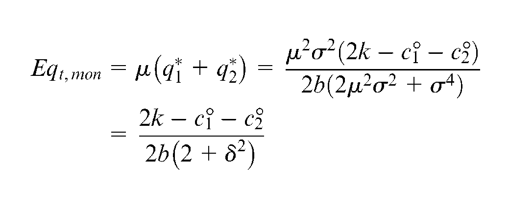
The case of cartel-monopoly
Duopoly manufacturers tend to form a combination of business organizations to control the market. For example, members of Organization of Petroleum Exporting Countries (OPEC), the well-known oil monopoly organization with cartel characteristics, aim to maximize their earnings by regulating their output. Prokop 25 considered the process of cartel formation in the industries characterized by collusive price leadership. Andaluz 26 analyzed the influence of the degree of differentiation on cartel sustainability, under both price and quantity competition in the context of a vertically differentiated duopoly. The literatures above mainly focused on the existence of cartel stability. In this section, we attempt to derive the best monopoly policy for the duopoly manufacturers and study the effect of random yield on market output. The duopoly firms would join up to maximize their total expected profit as follows
Their expected total profit can be maximized by deciding their target production set (q1,q2)
Theorem 3. Under random yield, there exists an optimal target production policy
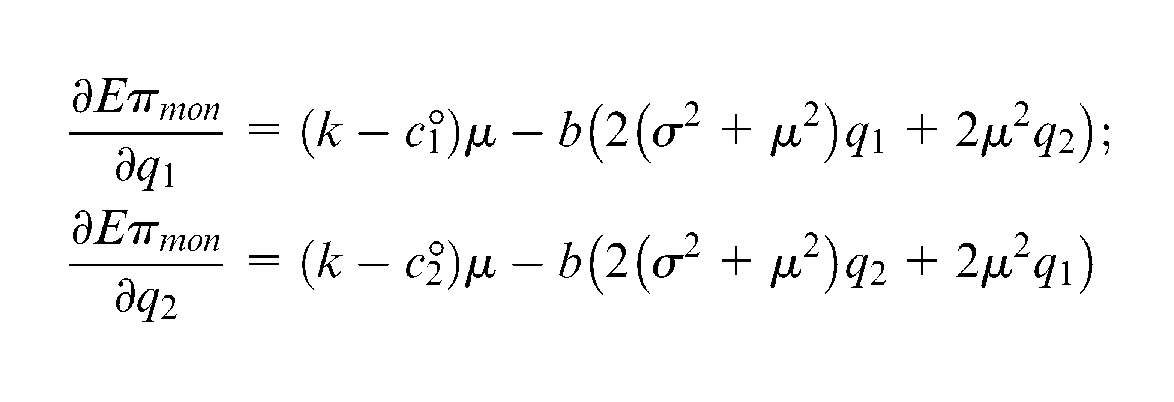
Proof. To derive the first-order condition of Eπmon with respect to q1 and q2, we have
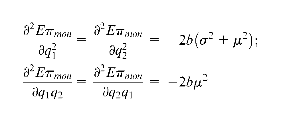
To derive the second order condition (soc) of Eπmon on q1 and q2, we have
The Hessian matrix is written as
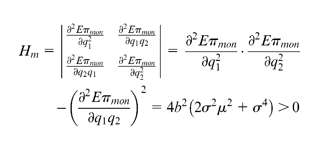
Because
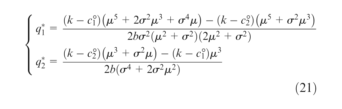
Proposition 3. In the monopoly case, manufacturer with lower cost owns a larger (expected) market share, that is, (i) if
Proof. Because
Lemma 6. (i) In the monopoly case, the expected market output decreases with δ and (ii) the expected market output under the monopoly case is smaller than the symmetric case, that is,
Proof of (i). This is similar to the proof of Lemma 1.
Proof of (ii). This is given by
As
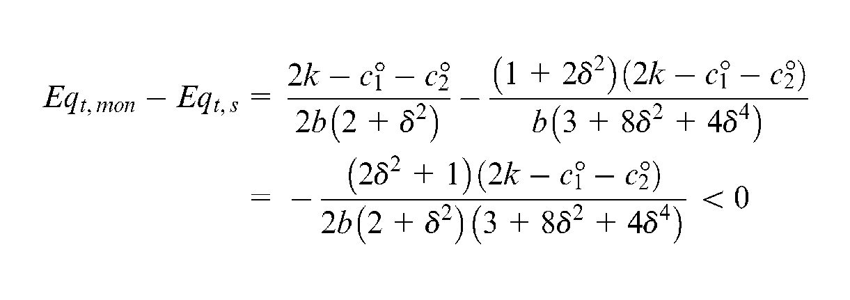
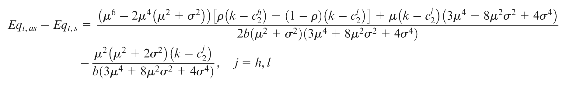
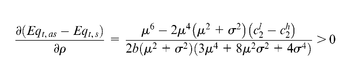
which proves (ii). Comparing the results with the asymmetric case and combining Lemma 6, we have
Lemma 7. (i) If M2 in the asymmetric case is low cost type, then there is
Proof of (i). Because
Proof of (ii). This is derived by solving the difference of
An extension: ρ is “made” and released by M2
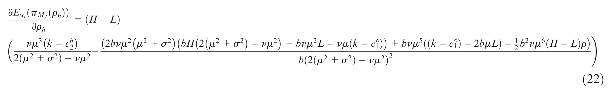
M2’s expected profit
In some activities of commercial and social politics, certain participants have the ability to release some information to confuse their competitor(s). Stronger participants may not only have superiority in getting access to important intelligence but also perform better in creating valuable information which can change their opponent’s decision-making. In a monopolistic market, the existing monopoly enterprise would like to pretend to be an extreme low cost type which will hold back the potential entry by threatening to launch a price war. Because cost c2 is not known to M1, M1’s production decision depends on the estimation of the probability of M2’s cost type. In many competitive industries, stronger firms tend to take actions and release some information to induce or confuse their opponent firm’s appraisal of her cost type or financial condition. We further assume that the probability that M1 considers M2’s cost type is gained by evaluating several pieces of marketing information which are formatted and released by the stronger M2. That is, ρ is “made” by M2. M2 could affect M1’s production decision by covertly controlling M1’s evaluation of ρ. Because M1 is not aware that ρ is “made” by M2, M2 could choose a best ρ by calculating M1’s best reaction function to maximize M2’s own expected profit function. To solve for the optimal condition of the high cost–type M2, for example, M2’s expected profit (from equation (13)) can be turned into
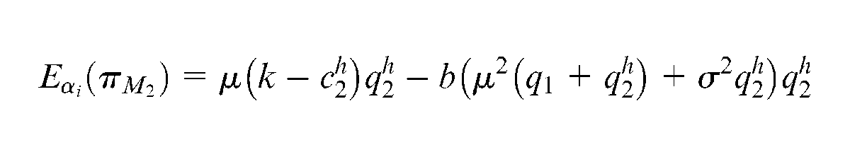
From equation (13), it could be found that the realization of
Proposition 4. The expected profit function of M2 is a convex function on the probability ρ.
Proof. Because M1 is not aware that her measurement of ρ is “made” by M2, the process of obtaining the optimal target production quantity equilibrium
To derive the second-order condition on ρ, we obtain
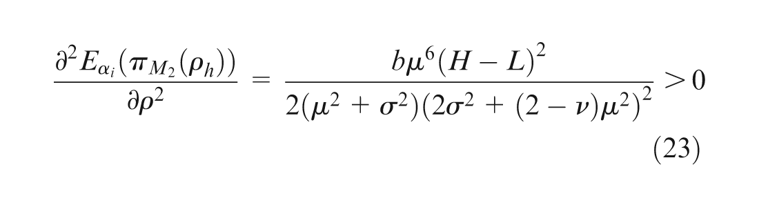
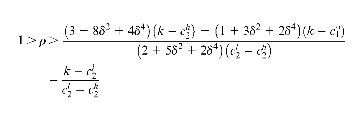
A same result can be reached when M2 is a low cost type. Thus, we can derive that there exists a unique ρ to minimize the expected profit function of M2. Recall in this section that ρ is decided by M2. For M2, the final realization of ρ depends on her market capability which she needs to monitor in order to make sure that M1 believes it. Because of that consideration, an extreme value of ρ (such as 0 or 1) cannot be believed by M1. Generally, we use [ρ1, ρ2] (0 < ρ1 < ρ2 < 1) to denote the probability interval that can be controlled by M2, and then, we have Proposition 5.
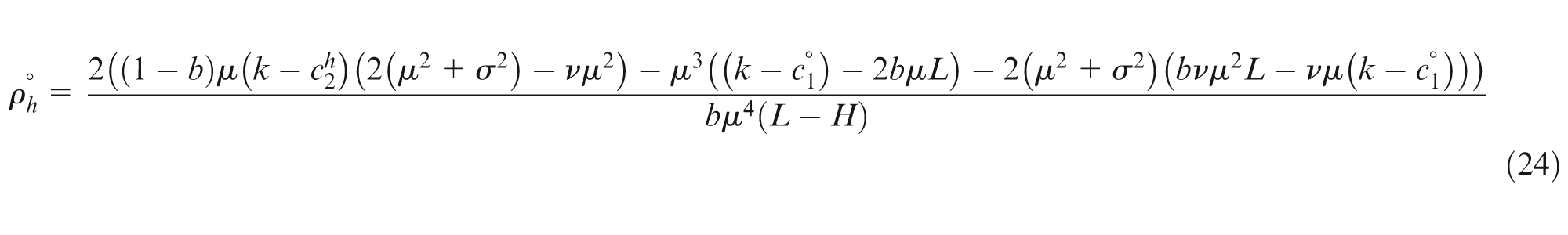
Proposition 5. To maximize the expected profit function, M2 should make her optimal decision as follows:
If
If
where ρh° stands for the extreme point of E(π2(ρ)). ρ* maximizes M2’s expected profit. By setting equation (14) equal to 0, and the “worst”ρ for M2 (high cost type) is given as follows
Proof of (i). If
Proof of (ii). This can be obtained similarly. For some examples of this phenomenon, see section “Numerical illustrations.”
Consumer surplus
Formally, when the production quantity is denoted as Q, then the expected consumer utility can be expressed as
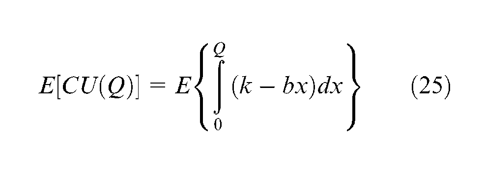
As the expected payment by the consumer is denoted as E[(k−bQ)Q], then the expected consumer surplus under random yield is given by
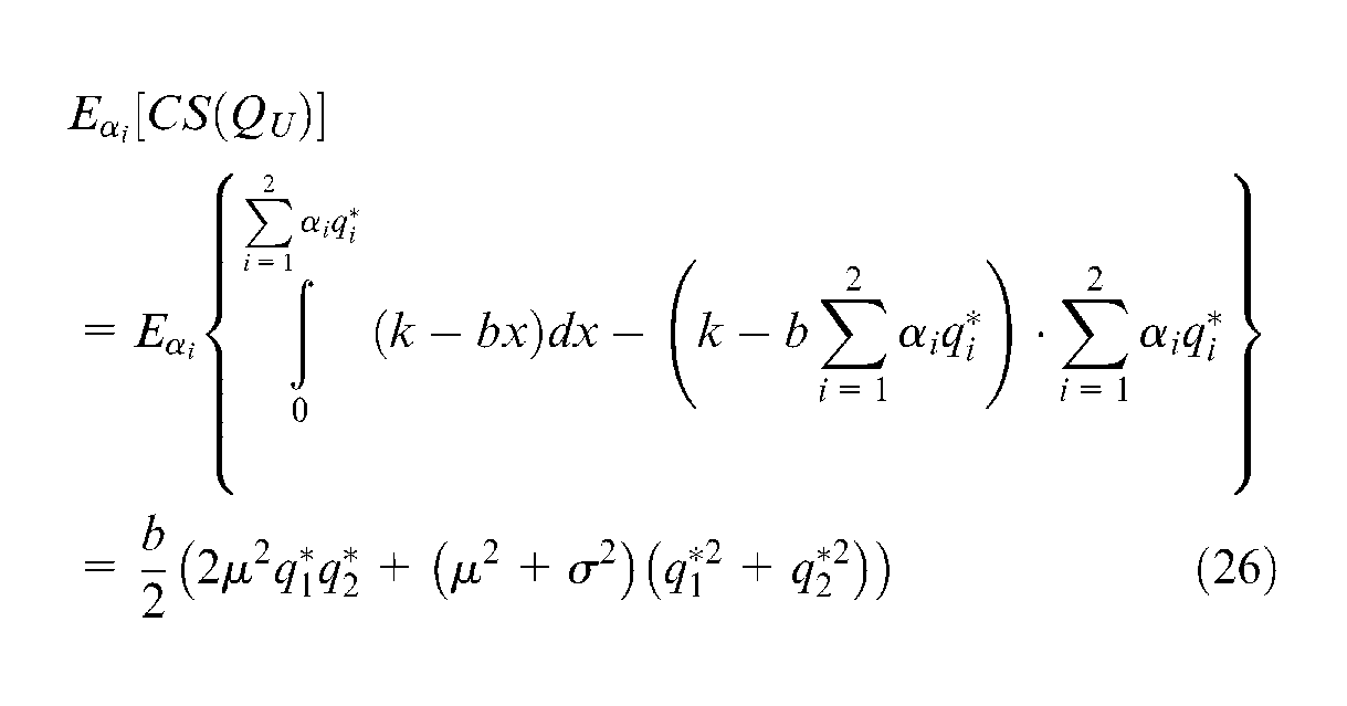
Proposition 6. The expected consumer surplus under asymmetric information is convex on ρ.
Proof. To derive the first-order condition of equation (26) on ρ, we have
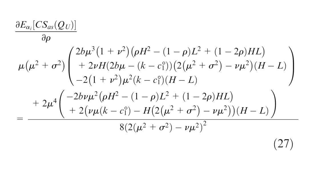
To derive the second-order condition on ρ, we obtain
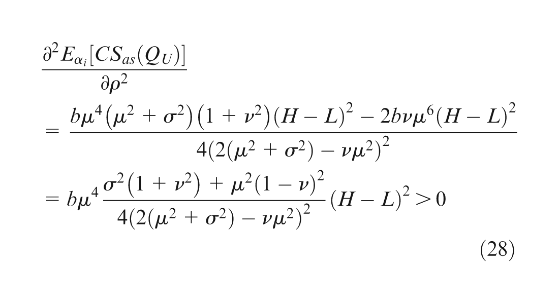
Equation (28) indicates that there exists a unique
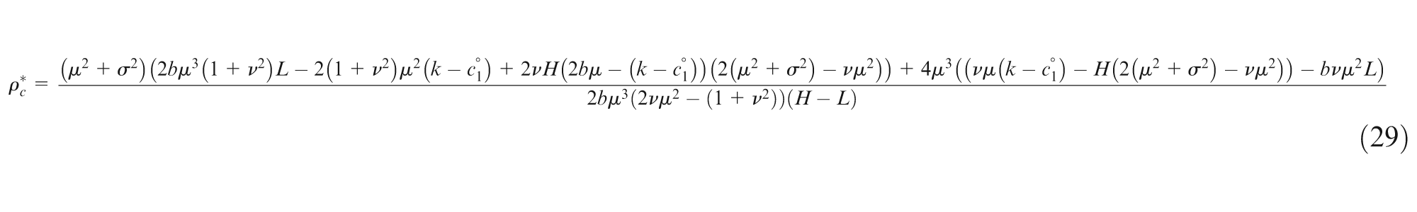
Based on Propositions 5 and 6, we derive that the optimization of M2’s expected profit is highly related to consumer surplus:
Proposition 7. The optimization of M2’s expected profit is highly related to the maximization of consumer surplus under asymmetric information:
If
If
If
If
Proof of (i) and (ii). If
Proof of (iii) and (iv). This is similar to the proof of (i) and (ii).
The results above can be used as a reason for government policies to control monopolistic behavior. To gain more insights into the results given above and the impact of yield uncertainty upon Cournot duopoly competition model, numerical examples are presented in the next section.
Numerical illustrations
We take the values of the parameters involved in the model as b = 0.52, k = 800, c11 = 0.93, c12 = 0.2,
In the following discussions, we assume that M2 is high cost type. To study the effect of yield uncertainty on the market, we draw Figure 2 to study the effect of yield uncertainty on the expected market output.
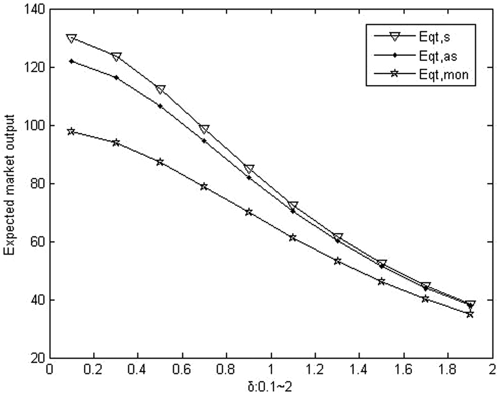
Comparison of expected market output in three cases when δ varies
From Figure 2, we can see that the expected market output of all three cases decreases when δ increases. The comparison shows that
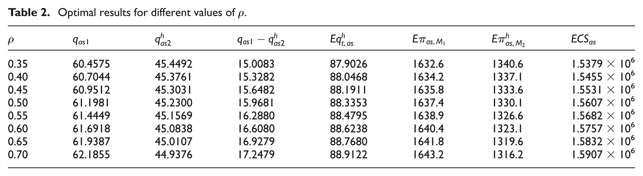
Table 2 explores the optimal production decisions when ρ is controlled by M2. From Table 2, it can be observed that qas1,
Optimal results for different values of ρ.
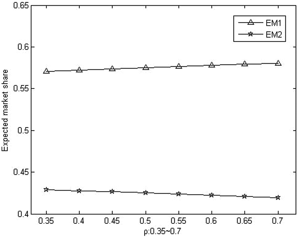
The effect of ρ on the duopolist’s expected market share.
Discussion and conclusion
The duopoly model with a Cournot form with yield randomness has received little attention. In this article, a Cournot duopoly production competition model was examined under random yield. The model was analyzed by giving the expectation value and variance of the random yield risk in a symmetric, asymmetric and monopoly environment, respectively. In a symmetric and asymmetric situation, we respectively derive that there exist a Nash and Bayes–Nash target production policies for the duopoly manufacturers. For the monopoly situation, an optimal production policy which could maximize their total expected profit was given.
The effect of yield uncertainty on the expected market output has been studied in each case. Regardless of the random yield and the competition environment, the unit production cost always plays a negative role in the manufacturers’ setting of a target production quantity, which is the same within the deterministic yield case. The comparison of the duopolist’s expected market share has been studied. We also compared the expected market output among the three situations. Then, we extended the asymmetric model by considering a powerful oligarch who can exert influence on her rival’s production decision by releasing her own cost-type information. We derive that the maximization of the stronger manufacturer’s expected profit is highly correlated with consumer surplus.
To the best of our knowledge, few researchers have studied the Cournot duopoly model under random yield. The model we analyzed is a static game. However, firms may compete in a dynamic way. Thus, it is necessary and worthwhile to extend our model in the future to study the case when the manufacturers play dynamically.
Footnotes
Declaration of conflicting interests
The authors declare that there is no conflict of interest.
Funding
The work was partly supported by the National Natural Science Foundation of China (71071113), PhD Programs Foundation of Ministry of Education of China (20100072110011) and the Fundamental Research Funds for the Central Universities.