Sage Journals: Discover world-class research

Abstract

Quality of machined surfaces and its integrity are strongly dependent on tool wear, which consequently depends on the tool life or machining time. Therefore, prediction of the machining time of the cutting tool during machining processes is very important in order to obtain high precision parts and to reduce manual fit operations and production cost. In this work, the relationship between texture features of the gray-level co-occurrence matrix and the machining time of the cutting tool in turning operations has been investigated, and the results show that four texture features are highly correlated with machining time. These highly correlated texture features were utilized to calculate machining time of the cutting tool from captured images of machined parts. The verification results showed that the maximum percentage of error between the actual and calculated machining time ranged between −4.65% and 7.79%.

Keywords

Turning operations machining time tool life computer vision image processing texture features

Introduction

Quality of machined surfaces and its integrity are strongly dependent on tool wear, which consequently depends on the tool life or machining time. When a cutting tool reaches its life end, it must be replaced before the cutting edge of the tool cannot produce the required surface quality and the accepted tolerance.¹ It was reported that tool wear/tool life increases by increasing the machining time of the cutting tool.^2,3 Therefore, the machining time of a cutting tool can be considered as an indicator to the tool wear and tool life. Because many parameters can affect the relationship between tool life and machining time such as cutting conditions, workpiece material, and lubrication, this article concentrates on the calculation of the machining time of cutting tools. The analysis of relationship between tool life and machining time using texture features could be studied in a further research.

In addition, tool life or the machining time of the cutting tool should be taken into consideration in order to complete finishing operation with just one tool, avoiding the intermediate stops in order to change the tool due to its wear.⁴ Eventually, sudden failure of cutting tools leads to loss of productivity, rejection of parts, and consequential economic losses.⁵

Estimation of tool wear/tool life and the corresponding economic analysis are among the most important topics in process planning and machining optimization.⁶ Prediction and detection of tool wear before the tool causes any damage on the machined surface are very significant to avoid loss of products, damage to the machine tools, and loss in productivity. For most researchers and tool manufacturers, tool wear progress and tool wear profile are also of the utmost importance.⁷

Experimentally, prediction of tool wear is performed by calculating tool life using empirical tool life equations such as Taylor’s equation as well as its extension versions. However, Taylor’s equations consume a lot of money and time⁸ since they give relatively reliable results only in a narrow cutting speed range.⁹

Many researches have been done to study the relationship between tool life and machining time and their effect on final products. For example, Narayana Rao et al.² studied the progress of tool wear with machining time and reported that initially tool wear is rapid and gets stabilized with progress in machining time. Dhar et al.¹⁰ studied the effect of machining time and tool wear on surface roughness of AISI 1060 steel obtained by turning process. They reported that R_a values have the tendency to increase with machining time and tool wear. Similarly, Mantana Srinang and Asa Prateepasen³ reported that tool wear increases by increasing machining time.

Similarly, many researches have been created to estimate or predict the tool life. For example, Erry Yulian et al.¹ developed a MATLAB Simulink model to estimate tool life during high-speed hard turning based on the relationship between the flank wear progress and time. Also, Tsai et al.¹¹ presented a network model for predicting tool life in high-speed milling (HSM) operations. They reported that experimental results have shown that the network model could be used to predict HSM end mill life under varying cutting conditions, and the prediction error of HSM tool life is less than 10%.

In the field of image processing and computer vision, image texture is considered an important feature, which provides important information for scene interpretation,¹² and it plays a crucial role in computer vision and pattern recognition. Statistical approaches define textures as stochastic processes and characterize them by a few statistical features. Haralick et al.’s¹³ texture features–based gray-level co-occurrence matrix (GLCM) is one of the most widely used techniques for texture analysis. It captures second-order gray-level information, which is mostly related to human perception and the discrimination of textures. GLCM texture features have proved their usefulness in a variety of image analysis applications.^14–17

Determination of tool wear using computer vision is fairly widespread in the manufacturing literature and dates back 30 years.¹⁸ Many texture descriptors were used for tool wear monitoring using computer vision. For example, Kassim et al.^19,20 used both fractal analysis and Hough transform in order to monitor tool wear of machined surfaces. Similarly, Li et al.²¹ used the Wavelet Packet for the same purpose. Volkan Atli et al.²² introduced a computer vision–based approach to monitor drilling tool condition by capturing images and applying a Canny edge detector to extract tool features from the acquired images. A comprehensive review of tool wear monitoring using computer vision has been introduced by Kerr et al.²³

In a previous work,²⁴ it was found that some GLCM texture features are highly correlated with surface roughness parameter R_a (arithmetic average height). The idea of this article came from these results. Therefore, the aim of this work is to investigate the relationship between GLCM texture features and the machining time of the cutting tool in turning operations in order to discover texture features that are highly correlated with the machining time. In turn, these texture features can be used to calculate the machining time of the cutting tools from captured images of machined parts.

Image texture features

Generally, the co-occurrence matrix, M_c(i, j), is calculated using the following equation

M_{c} (i, j) = \frac{P (i, j)}{\sum_{i, j}^{n} P (i, j)}

(1)

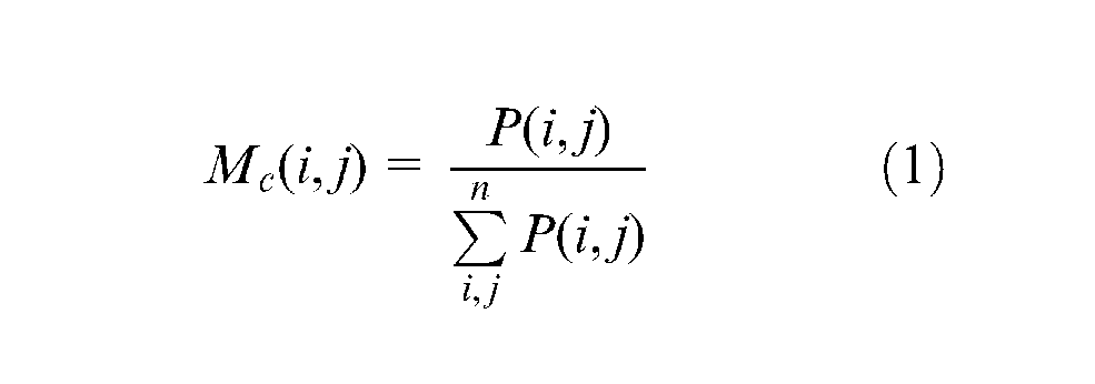
where M_c(i, j) is defined as the co-occurrence of gray level occurring; P(i, j) is the frequency of occurrence of gray levels i and j; and n refers to the total number of pixel pairs. A normalized matrix is produced by dividing each element of the GLCM by the summation of all elements.

A detailed explanation of the GLCM and its calculation method is presented in Gadelmawla.²⁴ All texture features that can be calculated from the GLCM (24 features) were collected from the literature and discussed in previous works.^25,26 These texture features were used in this work to calculate the machining time of the cutting tools from captured images of parts machined by turning operations.

Experimental work

This section describes the procedures that were applied to prepare the required specimens in order to investigate the relationship between the machining time of the cutting tool and the image texture features.

To prepare the required specimens, a cutting tool for turning operations with tips of commercial-type CNMG 120408EN-TM was utilized. A steel bar with 50 mm diameter (Steel 70 type) was used as a raw material to produce the required specimens. All specimens were machined using the same cutting conditions. It was decided to use the cutting tool for 4 h of actual cutting process to produce 10 cylindrical specimens with 50 mm diameter using face turning operations. To calculate the required length of each specimen, it was necessary to calculate the machining time of each specimen, the machining time of each face, and the depth of cut. The following sections show how to calculate the required length of each specimen.

Calculation of the specimen’s machining time

To calculate the length of machined part (l_m) of each specimen, it was required to calculate the machining time for each specimen (t_s) and the machining time for each face (t_f). As it was mentioned before, it was decided to use the cutting tool for 4 h to produce 10 specimens; the required machining time for each specimen (t_s) can be calculated using equation (2)

t_{s} = \frac{t_{t} \times 60}{n}

(2)

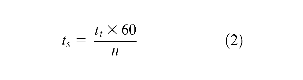
where t_s is the machining time required for each specimen (in min), t_t is the machining time for the cutting tool (in h) and n is the number of specimens to be machined by the cutting tool.

As a result, each specimen will be machined for 24 min (4 × 60/10). Because the machining process used in this work was a face turning operation, the machining time for each face (t_f) can be calculated using equation (3)

t_{f} = \frac{D}{2 fs}

(3)

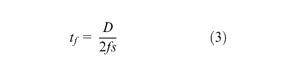
where t_f is the machining time required for each face (in min), D is the workpiece diameter (in mm), f is the feed (mm/rev) and s is the speed (r/min).

Calculation of specimen dimensions

Once the machining time for each specimen (t_s) and the machining time for each face (t_f) are calculated, the length of machined part (l_m) in each specimen can be calculated using equation (4)

l_{m} = \frac{t_{s}}{t_{f}} \times d_{c}

(4)

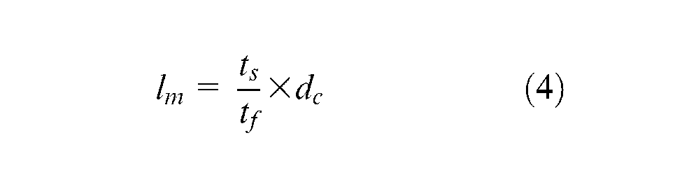
where l_m is the length of machined part (in mm), t_s is the machining time required for each specimen (in min), t_f is the machining time required for each face (in min) and d_c is the depth of cut (in mm).

By referring to Figure 1, the total length (l_t) of each specimen can be calculated using equation (5)

l_{t} = l_{w} + l_{m} + 2 l_{s}

(5)

where l_t is the total length of raw specimen (in mm), l_w is the length of workpiece after machining and before finishing (in mm), l_m is the length of machined part (in mm) and l_s is the length of each face to be straighten (in mm).

Figure 1.

Dimensions used to calculate the total length of row specimens.

In this case, the final length of workpiece (l_wf) can be calculated by equation (6)

l_{wf} = l_{w} - l_{f}

(6)

where l_f is the length of finishing process (in mm).

To calculate the dimensions of raw specimens based on different machining parameters, an Excel sheet has been created to automate this process as shown in Figure 2. Once the machining data and cutting conditions are entered by the user through the first two sections, the calculated dimensions for each specimen are displayed in the third section (calculated parameters), and it will be presented graphically at the right side of the Excel sheet. As shown in Figure 2, the calculated length of each specimen was 88 mm. Therefore, a steel bar with 50 mm diameter (Steel 70 type) was used as a raw material to produce 10 specimens with a length of 88 mm for each specimen. These specimens, then, were machined using a computer numerical control (CNC) machine as discussed in the following section.

Figure 2.

Excel sheet used to calculate the dimensions of raw specimens based on the cutting parameters.

Machining of specimens

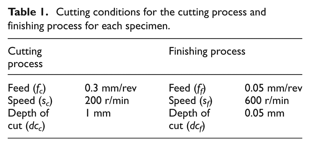
A CNC turning machine (Figure 3) was used to produce the required specimens, and a CNC part program was prepared to reduce the length of each specimen from 88 to 20 mm using the cutting conditions shown for the cutting process in Table 1. To get relatively smooth surfaces for each specimen, a finishing process was used to finish the face of each specimen using the same tool and the cutting conditions shown in the finishing process column of Table 1. In the finishing process, the speed is increased, while the feed and the depth of cut are decreased.

Figure 3.

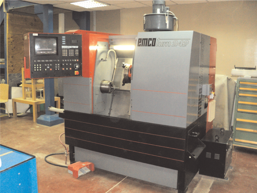
The CNC machine used to produce the investigated specimens.

Table 1.

Cutting conditions for the cutting process and finishing process for each specimen.

Cutting process		Finishing process
Feed (f_c)	0.3 mm/rev	Feed (f_f)	0.05 mm/rev
Speed (s_c)	200 r/min	Speed (s_f)	600 r/min
Depth of cut (dc_c)	1 mm	Depth of cut (dc_f)	0.05 mm

Capturing images

A Nikon ECLIPSE 150 industrial microscope with DS-Fi1 digital camera system (Figure 4) was used to capture images for machined specimens. The microscope was connected to a PC compatible computer with 3.0-GHz Pentium IV processor, 2 MB of memory and Windows XP operating system. The charge-coupled device (CCD) camera features a 5-megapixel CCD that captures at a high resolution of 2560 × 1920 pixels.

Figure 4.

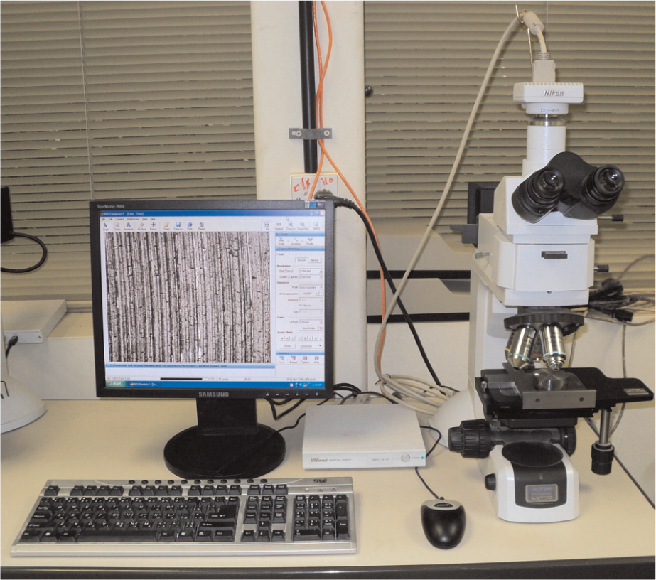
The vision system used to capture images.

A capturing image software called NIS is provided with the Nikon vision system, and it was used to capture images for all machined specimens. The NIS software enables to capture images with different sizes (up to resolution of 2560 × 1920 pixels). However, to speed up the calculation of images’ texture features, the CCD camera was adjusted to capture images of resolution 1280 × 960 pixels.

Adjusting location of specimens

It is well known that specimens machined by face turning operations have different textures at various radial distances. Therefore, capturing images at different radial distances might affect the results of the image analysis process. In order to capture images at the same radial distance for all specimens, a special fixture consisting of a square angle and block gauges was used. Figure 5 shows how to position specimens under the microscope using the square angle and block gauges. Also, Figure 6 shows a side view of the microscope to show how the block gauges were used to fix the microscope table at a specific position. As shown in Figure 5, the square angle was placed, so that one side touches the microscope table at the front and the other side touches the block gauges shown on left. Each specimen was set under the microscope, so that it touches the two sides of the square angle.

Figure 5.

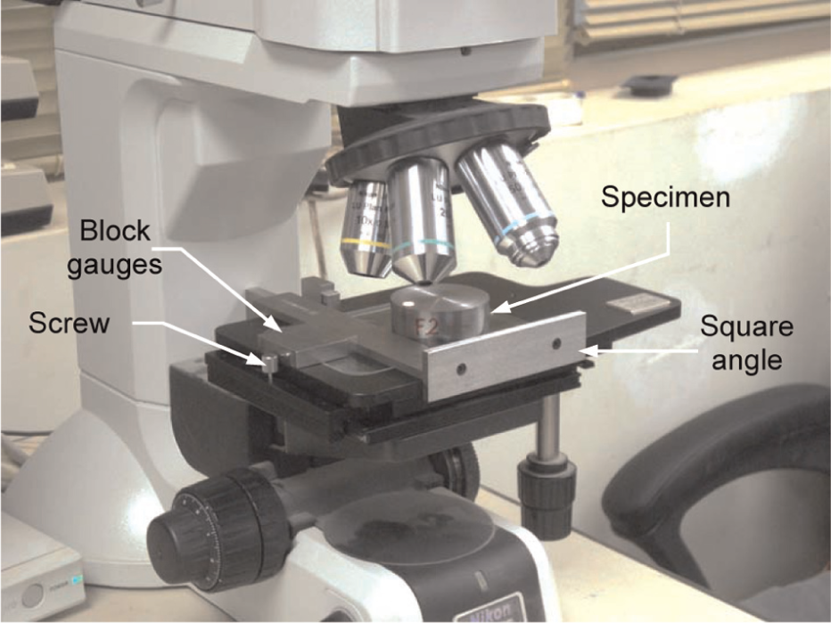
Using square angle and block gauges to control movement of the microscope table in X direction.

Figure 6.

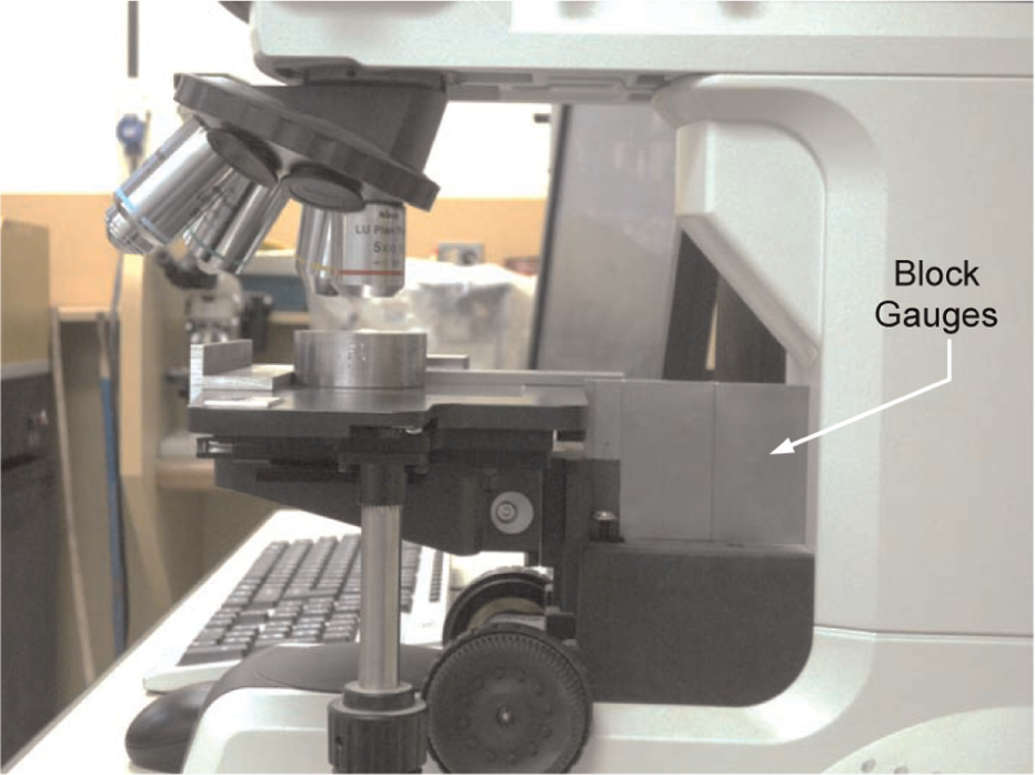
Using the block gauges to control the movement of the microscope table in Y direction.

Captured images

For each specimen, three different images were captured at the same radial distance. To avoid varying illumination conditions, which may affect the values of texture features, the microscope light was adjusted to constant light intensity while capturing all images. Figure 7 shows the captured images for the 10 machined specimens. All specimens were captured at a magnification of 5×.

Figure 7.

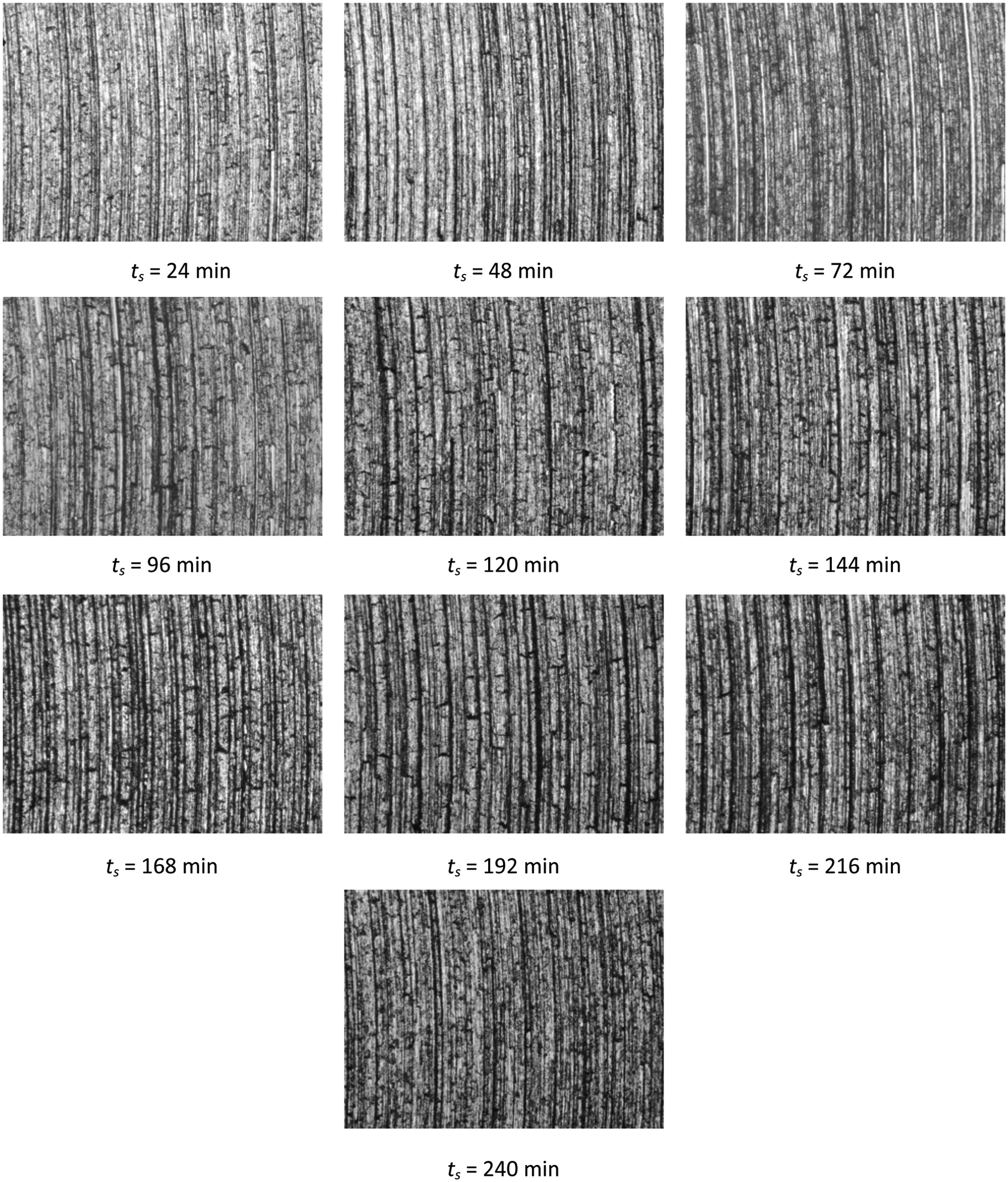
Captured images for the 10 specimens.

Image analysis

To calculate image texture features for captured images, a software named GLCMTF (GLCM Texture Features) was used. This software was fully developed in-house and has been discussed in a previous work.^24,26 It is capable of calculating all GLCM texture features, discussed in section “Image texture features,” for up to 100 position operators (direction θ and distance d) of the GLCM. The image texture features were calculated for captured images by the GLCMTF software as follows:

For each specimen, the three captured images were opened by the GLCMTF software, then the texture features were calculated for each image using a position operator of (1, 0) (i.e. distance = 1 and angle = 0).

For each texture feature, the average of the values obtained from the three images was calculated and recorded as shown in Table 2.

For each texture feature, the relationship between the t_s and the values of the texture feature was plotted to a graph using MS Excel.

The equation of correlation between t_s and each texture feature was obtained from Excel. These equations were used later to calculate the machining time of the cutting tool from captured images.

Table 2.

Calculated texture features for different machining time.

Feature	Machining time of each specimen t_s (min)
	24	48	72	96	120	144	168	192	216	240
ASM	6.30E−05	6.31E−05	6.60E−05	6.52E−05	6.70E−05	7.04E−05	7.01E−05	7.25E−05	7.23E−05	7.54E−05
CPR	1.80E+08	2.10E+08	2.10E+08	2.60E+08	1.90E+08	1.20E+08	1.90E+08	2.80E+08	2.10E+08	1.60E+08
CSH	−2.12E+05	−5.47E+04	−2.30E+05	3.66E+04	−2.17E+05	−1.88E+05	−1.26E+05	1.03E+04	1.14E+04	−2.23E+05
CVAR	0.46	0.412	0.388	0.429	0.382	0.362	0.384	0.3915	0.375	0.342
CON	555.7	564.7	590.8	574.6	585.1	612.2	623.6	611.2	613.4	606.7
COR	3.12E−04	3.37E−04	3.38E−04	3.31E−04	3.53E−04	3.61E−04	3.39E−04	3.39E−04	3.48E−04	3.81E−04
DM	465.948	445.965	468.595	452.93	455.839	464.621	480.416	476.004	478.218	461.48
DgVAR	3.66E−07	4.11E−07	3.77E−07	4.06E−07	3.84E−07	3.65E−07	3.50E−07	3.80E−07	3.75E−07	3.98E−07
DAVE	17.825	17.141	18.611	17.645	18.296	18.141	19.149	18.821	18.828	18.252
DENT	3.89	3.878	3.927	3.883	3.909	3.949	3.964	3.945	3.941	3.912
DVAR	9.93E+05	9.78E+05	9.77E+05	9.63E+05	9.62E+05	9.60E+05	9.61E+05	9.44E+05	9.49E+05	9.35E+05
DIS	17.567	17.141	18.611	17.645	18.296	19.141	19.149	18.821	18.828	17.952
ENT	9.755	9.747	9.747	9.738	9.745	9.737	9.732	9.735	9.735	9.731
IDM	0.068	0.067	0.065	0.067	0.064	0.064	0.063	0.065	0.063	0.063
MaxP	1.95E−04	2.25E−04	2.38E−04	4.37E−04	2.13E−04	2.30E−04	1.70E−04	3.81E−04	2.87E−04	2.52E−04
MEAN	130.2	125.5	132.6	129.2	138.3	136.3	133.4	134.8	137.3	145.9
MCOR1	1.73E−01	1.69E−01	1.54E−01	1.67E−01	1.49E−01	1.34E−01	1.38E−01	1.56E−01	1.57E−01	1.34E−01
MCOR2	1.0677	1.0424	0.9468	0.9942	0.9203	0.8584	0.8512	0.9221	0.9690	0.8895
SDM	8.762	8.571	9.205	8.822	9.148	9.27	9.474	9.411	9.414	9.226
SIM	0.132	0.134	0.128	0.133	0.126	0.127	0.125	0.127	0.127	0.126
SAVR	22,881	22,558	22,810	22,342	22,519	22,334	22,414	21,913	21,713	21,627
SENT	1009	1005	1006	1001	999	1001	999	995	996	992
SVAR	567,364	559,248	557,024	537,828	535,690	537,103	536,176	519,148	518,564	505,230
VAR	2974	3073	2710	3026	2599	2524	2628	2823	2745	2481

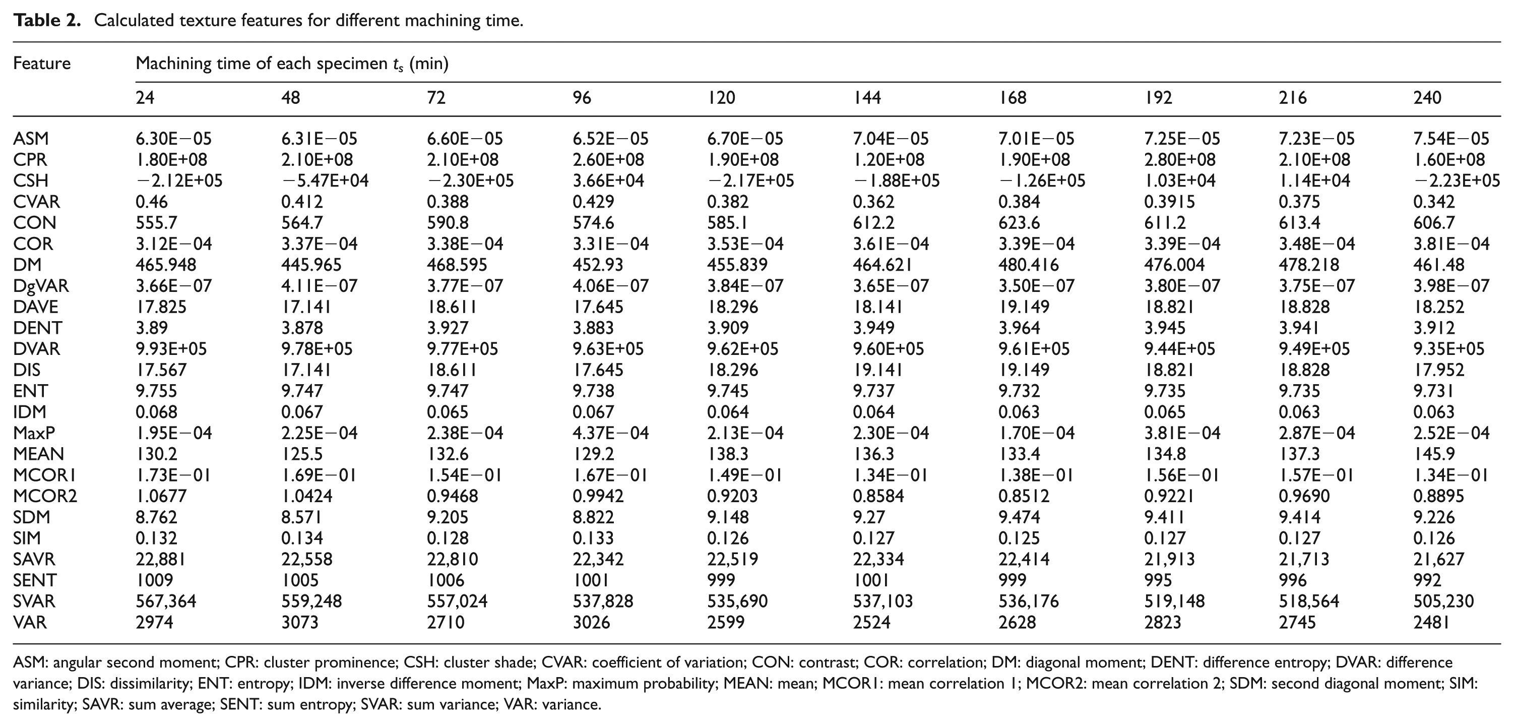
ASM: angular second moment; CPR: cluster prominence; CSH: cluster shade; CVAR: coefficient of variation; CON: contrast; COR: correlation; DM: diagonal moment; DENT: difference entropy; DVAR: difference variance; DIS: dissimilarity; ENT: entropy; IDM: inverse difference moment; MaxP: maximum probability; MEAN: mean; MCOR1: mean correlation 1; MCOR2: mean correlation 2; SDM: second diagonal moment; SIM: similarity; SAVR: sum average; SENT: sum entropy; SVAR: sum variance; VAR: variance.

Results and discussion

This section describes the correlations between the machining time t_s and all texture features. In addition, the process of calculating t_s from the captured images using texture features has been discussed.

Correlations between texture features and the machining time

Using Table 2, the correlation coefficient between the values of each texture feature and the values of t_s was calculated using equation (7)

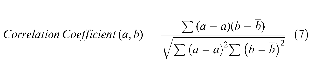
Correlation Coefficient (a, b) = \frac{\sum (a - \bar{a}) (b - \bar{b})}{\sqrt{{\sum (a - \bar{a})}^{2} {\sum (b - \bar{b})}^{2}}}

(7)

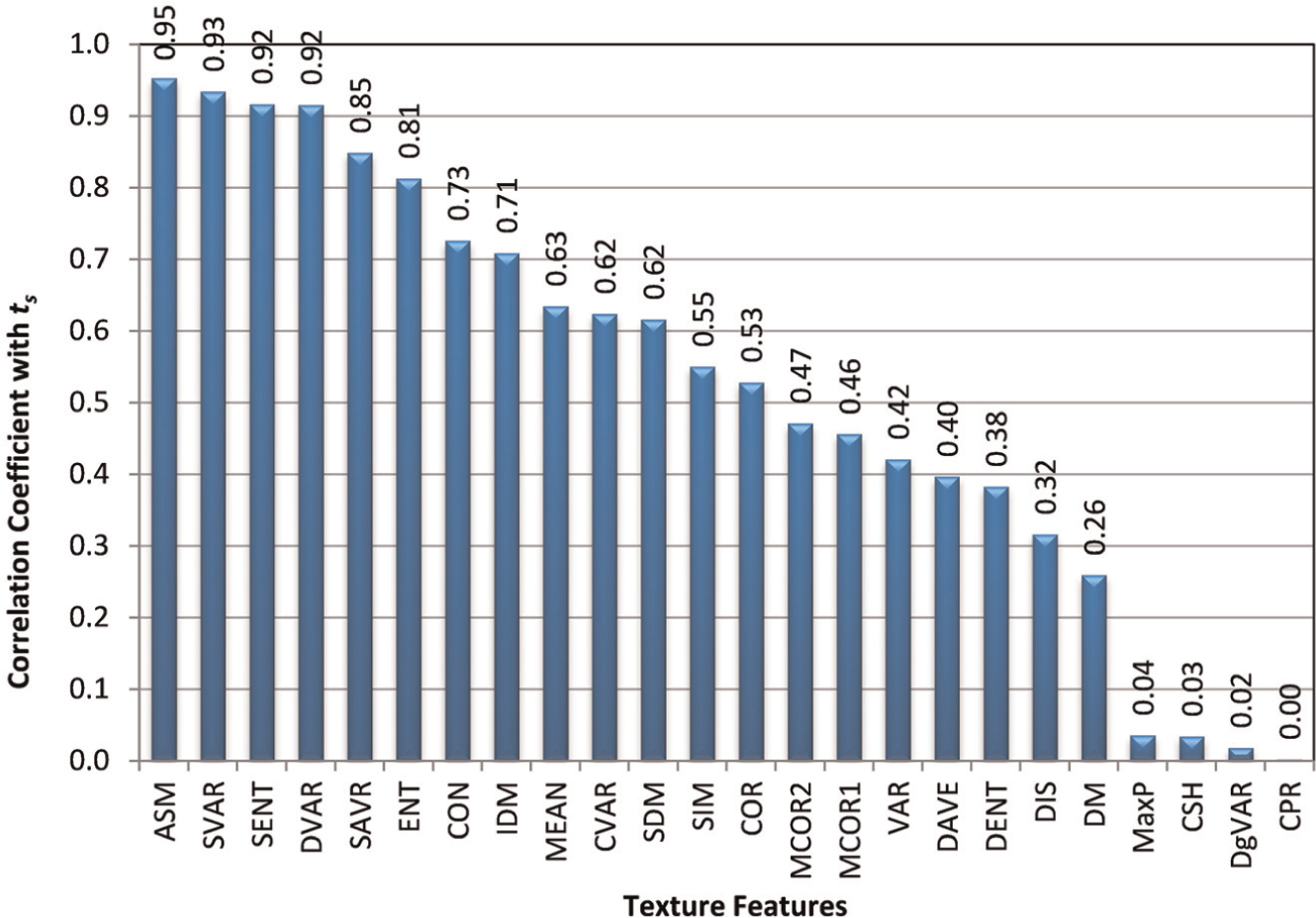
where a and b are the data sets of t_s and texture features, respectively, and $\bar{a}$ and $\bar{b}$ are the averages of t_s and the texture features data sets, respectively. Figure 8 shows the correlation coefficients of all texture features with t_s. The texture features are sorted in descending order according to their correlation coefficients with t_s.

Figure 8.

Texture features sorted according to their correlation coefficients with the machining time.

The following points could be observed from Figure 8:

Four texture features (angular second moment (ASM), sum variance (SVAR), sum entropy (SENT), and difference variance (DVAR)) are highly correlated with t_s (correlation coefficient greater than or equal to 0.9). Therefore, these texture features could be used to predict the value of t_s later on. Figure 9 shows the relationship between these texture features and t_s. The equation of correlation between each texture feature and t_s is also shown in the figure.

Two texture features (sum average (SAVR) and entropy (ENT)) are relatively highly correlated with t_s (correlation coefficient ranges between 0.8 and 0.9). Figure 10 shows the relationship between these texture features and t_s.

Other texture features do not have good correlation with t_s (correlation coefficient less than 0.80). Figure 11 shows the relationship between two of the texture features (dissimilarity (DIS) and diagonal moment (DM)) and t_s.

Texture features maximum probability (MaxP), cluster shade (CSH), Diagonal Variance (DgVAR), and cluster prominence (CPR) have approximately no correlation with t_s.

Figure 9.

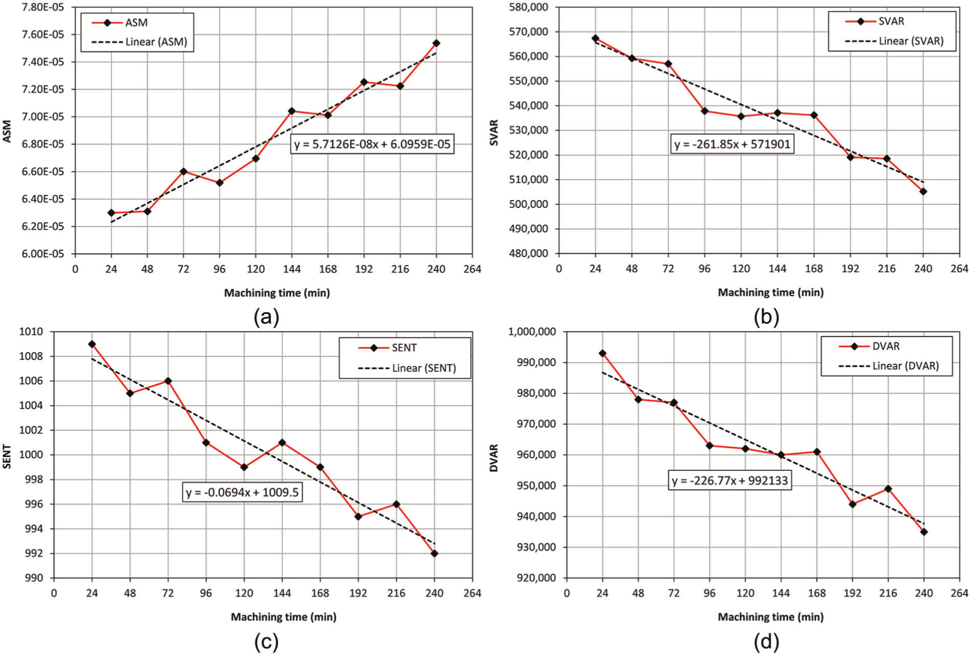
Relationship between highly correlated texture features and the machining time (correlation coefficient ≥ 0.90): (a) ASM (correlation coefficient = 0.95), (b) SVAR (correlation coefficient = 0.93), (c) SENT (correlation coefficient = 0.92), and (d) DVAR (correlation coefficient = 0.92).

Figure 10.

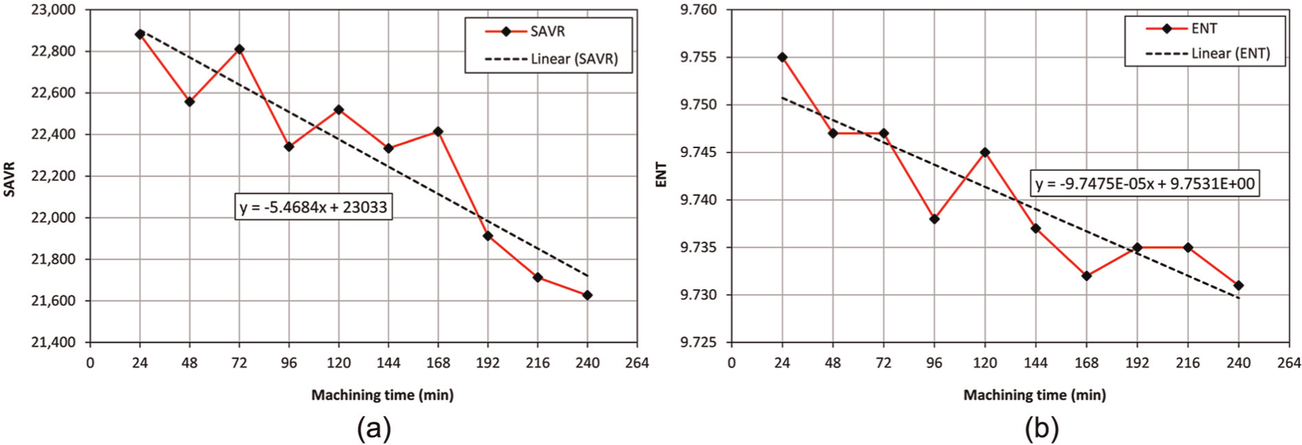
Relationship between some texture features of relatively high correlation and the machining time (correlation coefficient ranges between 0.80 and 0.90): (a) SAVR (correlation coefficient = 0.85) and (b) ENT (correlation coefficient = 0.81).

Figure 11.

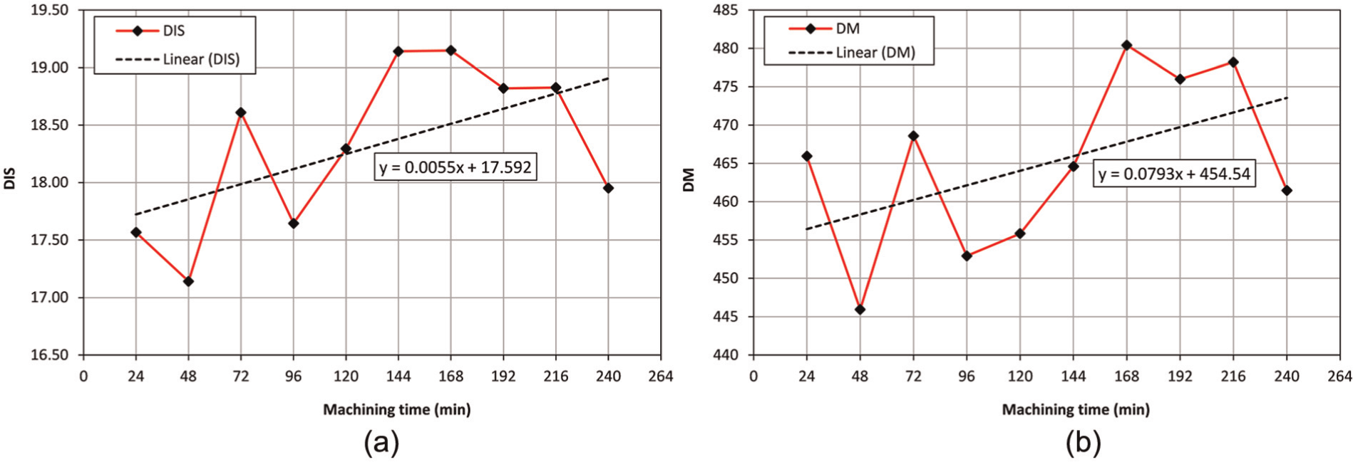
Relationship between some texture features of lowest correlation and the machining time (correlation coefficient less than 0.80): (a) DIS (correlation coefficient = 0.32) and (b) DM (correlation coefficient = 0.26).

Calculation of the machining time

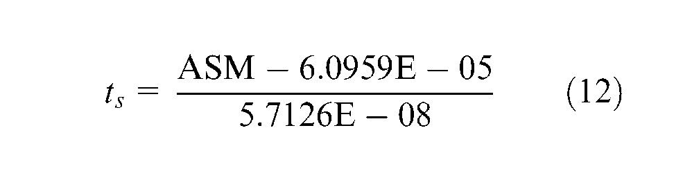
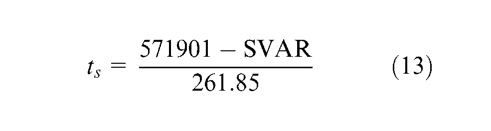
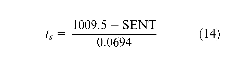
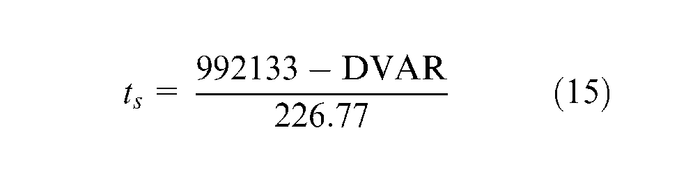
Regarding the equations shown in the plotted graphs (Figures 9 –11), y represents the texture feature and x represents the machining time t_s. From the plotted graphs, it can be seen that the equations of correlation for texture features that have high correlation with t_s are as follows

ASM = 5.7126 E - 08 t_{s} + 6.0959 E - 05

(8)

SVAR = - 261.85 t_{s} + 571901

(9)

SENT = - 0.0694 t_{s} + 1009.5

(10)

DVAR = - 226.77 t_{s} + 992133

(11)

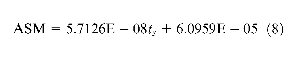
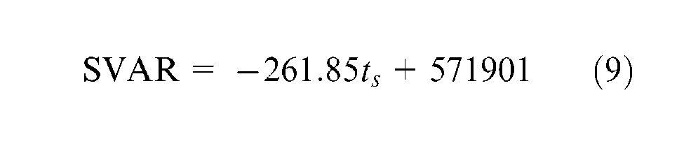
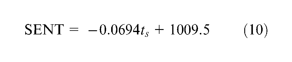
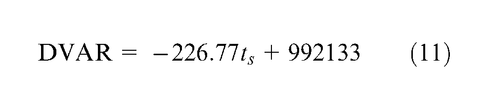
From these equations, the machining time can be calculated using one of the following equations

t_{s} = \frac{ASM - 6.0959 E - 05}{5.7126 E - 08}

(12)

t_{s} = \frac{571901 - SVAR}{261.85}

(13)

t_{s} = \frac{1009.5 - SENT}{0.0694}

(14)

t_{s} = \frac{992133 - DVAR}{226.77}

(15)

System calibration

To calculate the machining time t_s from captured images of machined parts based on the values of their texture features, the system should be calibrated. The calibration process can be done by entering the equations of calculating the machining time to the GLCMTF software. After that, when any image is opened, the software calculates its texture features and then substitutes by their values in these equations to calculate the machining time.

To perform the calibration process, a new module called machining time calculation (MTC) has been added to the GLCMTF software. The MTC module was written using visual C++, and it contains two dialog boxes. The first dialog box, Figure 12, is used to enter the equations used to calculate t_s (equations (12)–(15)) to the MTC module, which stores them to a file for further use by the software. The second dialog box, Figure 13, is used to display the calculated texture features and the calculated machining time for captured images of machined parts.

Figure 12.

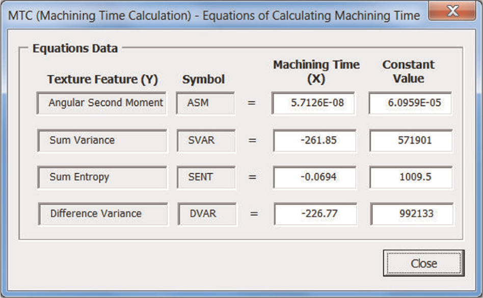
Entering equations of calculating the machining time to the MTC module.

Figure 13.

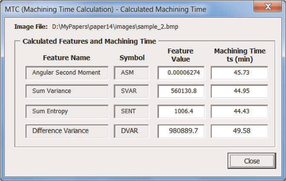
Calculated texture features and the machining time for sample 2 (after 48 min).

System verification

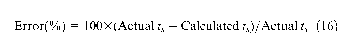
To verify the accuracy of the introduced system, the MTC module was used to calculate the machining time for three specimens of the samples produced during this work. The actual machining times for the selected specimens were 48, 120, and 192 min. A random image was captured for each specimen using the same fixture discussed in section “Adjusting location of specimens.” The MTC module was used to calculate the texture features and the machining time for each image, and the results were listed in Table 3. Table 3 also shows the percentage of error between the actual machining time and the calculated machining time. The percentage of error was calculated using equation (16) as follows

Error (%) = 100 \times (Actual t_{s} - Calculated t_{s}) / Actual t_{s}

(16)

Table 3.

Comparison between the actual and calculated machining time for three selected samples.

Texture feature	Sample 2			Sample 5			Sample 8
	Actual machining time = 48 min			Actual machining time = 120 min			Actual machining time = 192 min
	Feature value	Calculated t_s	Error (%)	Feature value	Calculated t_s	Error (%)	Feature value	Calculated t_s	Error (%)
ASM	0.00006274	45.73	4.73	0.00006681	113.43	5.47	0.00007108	184.65	3.83
DVAR	560,130.8	44.95	6.35	539,017.9	125.58	−4.65	524,278.3	181.87	5.28
SVAR	1006.4	44.43	7.44	1001.8	110.65	7.79	997.0	180.45	6.02
SENT	980,889.7	49.58	−3.29	966,542.0	112.85	5.96	947,103.3	198.57	−3.42

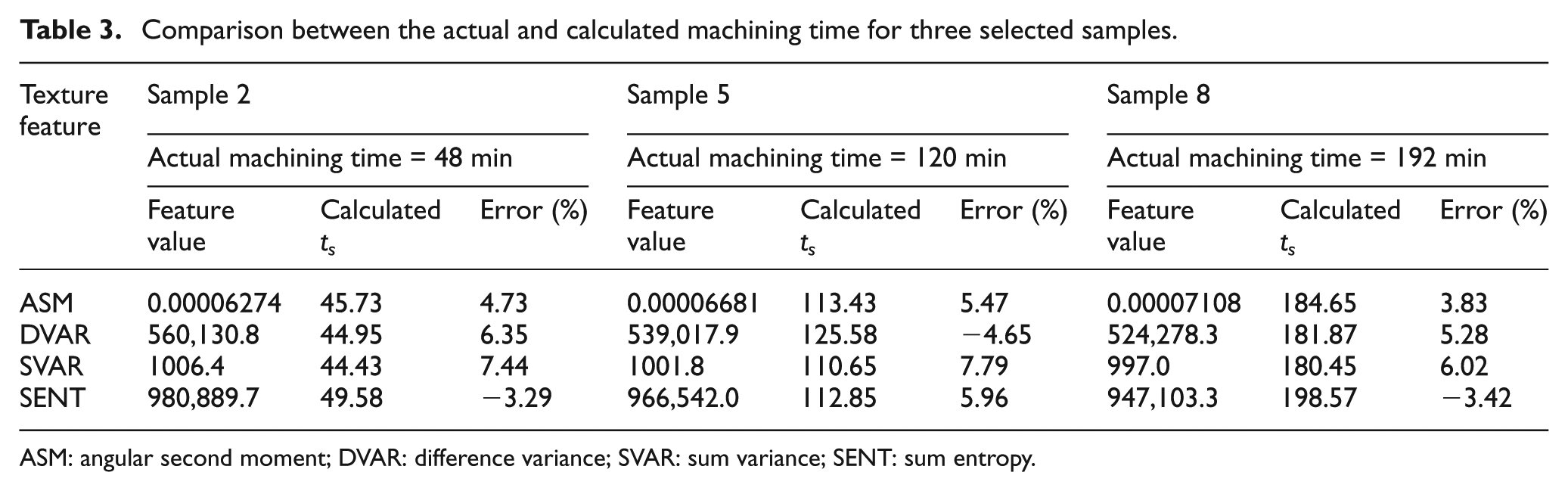
ASM: angular second moment; DVAR: difference variance; SVAR: sum variance; SENT: sum entropy.

From Table 3, it can be seen that the maximum percentage of error between the actual and calculated machining time was from 3.83% to 5.47% for ASM, from −4.65% to 6.35% for DVAR, from 6.02% to 7.79% for SVAR, and from −3.42% to 5.96% for SENT. In general, the maximum percentage of error between the actual and calculated machining time for the four texture features was from −4.65% to 7.79%. According to this study, ASM gave the best results.

System limitations

As it was mentioned in a previous work,²⁴ changes in illumination conditions while capturing images may affect the values of texture features. On the other hand, it is well known that vision systems are usually utilized to perform a particular task in specific circumstances. If these circumstances change, the vision system should be recalibrated. The calibration process here means that texture features that have high correlation with t_s should be discovered and their equations of correlation should be recalculated and entered into the MTC module. This makes the employed vision system suitable for calculating machining time of cutting tools in mass production for specific machining operation.

Conclusion

In this work, the relationship between GLCM texture features and the machining time of cutting tools in CNC face turning operations has been investigated. The following points could be concluded:

It was found that four texture features (ASM, SVAR, SENT, and DVAR) have high correlation factor (>0.9) with the machining time of cutting tools. Therefore, these texture features could be employed to calculate the machining time from captured images of machined parts.

It was found that ASM has the highest correlation factor (0.95) among the four texture features. Also, it was found that ASM is proportionally increased by increasing the machining time.

While ASM is proportionally increased by increasing the machining time, it was found that the other three texture features (SVAR, SENT, and DVAR) are proportionally decreased by increasing the machining time. However, they give a good correlation with the machining time (≥0.92).

Two texture features (SAVR and ENT) are relatively highly correlated with the machining time (correlation coefficient ranges between 0.8 and 0.9). Other texture features do not have good correlation with the machining time (correlation coefficient less than 0.80). Therefore, these features cannot be used to calculate the machining time of the cutting tool.

The verification of the proposed system showed that the maximum percentage of error between the actual and calculated machining time for the four texture features ranges from −4.65% to 7.79%. Also, ASM gave the best results (maximum error ranges from 3.83% to 5.47%).

Footnotes

Appendix 1 Conflict of interest statement

The authors declare that there is no conflict of interest.

Funding

This research has been funded by the Scientific Research Deanship at Qassim University, KSA.

References

Erry Yulian

Muataz

Hazza

Muhammad

. Tool life estimation model based on simulated flank wear during high speed hard turning. Eur J Sci Res 2010; 39(2): 265–278.

Narayana Rao

Satyanarayana

Venkatasubbaiah

. Experimental estimation of tool wear and cutting temperatures in MQL using cutting fluids with CNT inclusion. Int J Eng Sci Tech 2011; 3(4): 2928–2931.

Srinang

Prateepasen

. Coherence function model for tool wear monitoring. Songklanakarin J Sci Technol 2008; 30(1): 93–99.

Lopez

Lacalle

Lamikiz

Sanchez

. Improving the surface finish in high-speed milling of stamping dies. J Mater Process Tech 2002; 123: 292–302.

Palanisamy

Rajendran

Shanmugasundaram

. Prediction of tool wear using regression and ANN models in end-milling operation. Int J Adv Manuf Tech 2008; 37(1–2): 29–41.

Balaji

. Performance-based predictive models and optimization methods for turning operations and application: part 1—tool wear/tool life in turning with grooved tools. J Manuf Process 2006; 8(1): 54–66.

Ozel

Nadgir

. Prediction of flank wears by using back propagation neural network modeling when cutting hardened H-13 steel with chamfered and honed CBN tools. Int J Mach Tool Manu 2002; 42: 287–297.

Mehrban

Naderi

Panahizadeh

. Modeling of tool life in using process using experimental method. Int J Mater Form 2008; 1(1): 559–562.

Mamalis

Kundrak

Horvath

. Wear and tool life of CBN cutting tools. Int J Adv Manuf Tech 2002; 20: 475–479.

10.

Dhar

Ahmed

Khoda

AKMB

. Analysis of influence of machining time and tool wear on surface roughness in turning AISI-1060 steel. In: Proceedings of the international conference on mechanical engineering 2007 (ICME2007), Dhaka, Bangladesh, 29–31 December 2007. Publication and Technical Sub Committee, ICME2007.

11.

Tsai

Lee

. A predicted modeling of tool life of high-speed milling for SKD61 tool steel. Int J Adv Manuf Tech 2005; 26: 711–717.

12.

Briones

Aguilera

Brown

. Effect of surface topography on color and gloss of chocolate samples. J Food Eng 2006; 77(4): 776–783.

13.

Haralick

Shanmugam

Dinstein

. Textural features for image classification. IEEE T Syst Man Cyb 1973; 3: 610–621.

14.

Carfagni

Furferi

Governi

. A real-time machine-vision system for monitoring the textile raising process. Comput Ind 2005; 56(8–9): 831–842.

15.

Chandraratne

Samarasinghe

Kulasiri

. Prediction of lamb tenderness using image surface texture features. J Food Eng 2005; 28: 1–8.

16.

Tahir

Bouridane

Kurugollu

. An FPGA based coprocessor for GLCM and Haralick texture features and their application in prostate cancer classification. Analog Integr Circ S 2005; 43: 205–215.

17.

Iivarinen

Heikkinen

Rauhamaa

. A defect detection scheme for web surface inspection. Int J Pattern Recogn Artif Intell 2000; 14(6): 735–755.

18.

Otieno

Pedapati

Wan

. Imaging and wear analysis of micro-tools using machine vision. In: Proceedings of the international conference on engineering & technology (IJME-Intertech), Kean University, Union, NJ, New Jersey, USA, 19–21 October 2006, IT 301: Paper #071.

19.

Kassim

Mian

Mannan

. Texture analysis using fractals for tool wear monitoring. IEEE 2002; 3: 105–108.

20.

Kassim

Mian

Mannan

. Connectivity oriented fast Hough transform for tool wear monitoring. Pattern Recogn 2004; 37: 1925–1933.

21.

P-Y

Hao

C-Y

Zhu

S-W

. Machining tools wear condition detection based on wavelet packet. In: Proceedings of the sixth international conference on machine learning and cybernetics, Hong Kong, China, 19–22 August 2007, Volume 3, pp.1559–1564. Digital Object Identifier: 10.1109/ICMLC.2007.4370393.

22.

Volkan Atli

Urhan

Ertürk

. A computer vision-based fast approach to drilling tool condition monitoring. Proc IMechE, Part B: J Engineering Manufacture 2006; 220: 1409–1415.

23.

Kerr

Pengilley

Garwood

. Assessment and visualization of machine tool wear using computer vision. Int J Adv Manuf Tech 2006; 28(7–8): 781–791.

24.

Gadelmawla

. Estimation of surface roughness of turning operations using image texture features. Proc IMechE, Part B: J Engineering Manufacture 2011; 225(8): 1281–1292.

25.

Gadelmawla

. A vision system for surface roughness characterization using the gray level co-occurrence matrix. NDT&E Int 2004; 37: 577–588.

26.

Gadelmawla

Eladawi

Abouelatta

. Investigation of the cutting conditions in milling operations using image texture features. Proc IMechE, Part B: J Engineering Manufacture 2008; 222(11): 1395–1404.

Calculation of the machining time of cutting tools from captured images of machined parts using image texture features

Abstract

Keywords

Introduction

Image texture features

Experimental work

Calculation of the specimen’s machining time

Calculation of specimen dimensions

Machining of specimens

Capturing images

Adjusting location of specimens

Captured images

Image analysis

Results and discussion

Correlations between texture features and the machining time

Calculation of the machining time

System calibration

System verification

System limitations

Conclusion

Footnotes

Appendix 1

Conflict of interest statement

Funding

References