Sage Journals: Discover world-class research

Abstract

Geometric deviations are observable on every manufactured part since manufacturing processes are inherently imprecise and measuring processes always involve uncertainties. These geometric deviations have influences on the function and the quality of the product. Therefore, allowable limits for these geometric deviations, depicted as geometric tolerances, have to be set. They define the allowable geometric deviations of a part for which the product function is guaranteed. In this context, elastic deformations and the structural performance are key aspects. However, the manufacturing-caused geometric deviations have an influence on the elastic deformations during use and the structural performance of the parts. In other words, there are interdependencies between geometric deviations and elastic deformations which affect the dimensional accuracy of a loaded part in an assembly. Therefore, this article proposes an approach for determining the impact of geometric deviations on the structural performance. This approach employs techniques such as sensitivity analysis, analysis of robustness and evaluation of reliability, and aims at providing information about the expectable elastic deformations and structural performance to geometric tolerancing. It can be concluded that geometric deviations can have a big impact on the structural performance, and thus, not only parametric deviations but also geometric deviations regarding the form and shape of a part itself should be taken into account within the structural performance analysis and tolerance simulations.

Keywords

Structural performance computer-aided tolerancing geometric deviations

Structural performance evaluation in computer-aided tolerancing

Since every manufacturing process is inherently imprecise and every measuring process involves uncertainties, geometric deviations are generally observable on every manufactured and measured part.¹ These geometric imperfections can have huge influences on the function and the customer-perceived quality of the product. Hence, geometric dimensioning and tolerancing is an important step in the product development process since it is the step where the limits of allowable geometric deviations are defined. However, it is difficult to set these limits since geometric deviations influence the functional behaviour of the part in many ways. The structural performance, however, is a key aspect. Therefore, an approach is proposed that helps to determine the effects of geometric deviations on the structural performance.

By connecting different methods of computer-aided design (CAD), computer-aided tolerancing and tools for computer-aided simulations such as the finite–element (FE) method and assembly simulations, the product developer can be supported in setting the tolerance requirements. In this respect, the main goal is to draw a realistic virtual image of the geometry, function and behaviour of the real part or assembly group with geometric deviations during product development which facilitates the tolerancing activities.

The engineering design tasks in geometric tolerancing are mainly the tolerance specification, the tolerance allocation and the tolerance analysis (see Figure 1).² During the tolerance specification, kinds of tolerances that are useful and required for assuring the product function have to be identified. In the next step, the tolerance allocation, values for the selected kinds of tolerances have to be set. These values are then analysed with respect to the functional requirements and the emerging product costs during the tolerance analysis. If it can be found that the part does not fulfil the requirements, then the tolerance allocation and maybe even the tolerance specification have to be repeated, that is, the highlighted tolerance activities have to be carried out iteratively.

Figure 1.

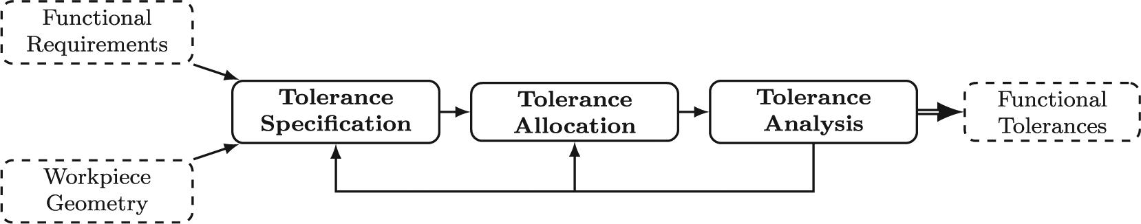
The computer-aided tolerancing process.

Since these tolerancing activities should be part of a complete and coherent tolerancing process,³ a unified language of geometric deviations and tolerances as well as models for their representation have to be employed. This need has led to the development of GeoSpelling as a coherent model for geometrical product specification (GPS),⁴ as well as several models for the representation of dimensions and tolerances such as the model of technologically and topologically related surfaces (TTRS) by Desrochers and Clément,⁵ the direct linearization method by Chase et al.⁶ or the deviation domain based on the small displacement torsor by Giordano et al.,⁷ among many others. These models aim at enabling the product developer to analyse the effects of geometric part tolerances on assembly gaps and clearances as well as, of course, the product function. However, these approaches model geometric tolerances but not observable geometric deviations in a true sense and make thus severe simplifications as far as workpiece imperfections are concerned.^8,9

Furthermore, various concepts and models for the exchange of product data especially tolerances and assembly information in all product lifecycle management tools, for example, for integrated measurement processes, have been proposed such as a model based on XML by Zhao et al.,¹⁰ the open assembly model by Baysal et al.¹¹ or an integrated modelling method based on key features and graph theory proposed by Zhang et al.¹²

However, during tolerance analysis, the question whether all parts within tolerance fulfil their requirements regarding the structural performance has to be answered. More than 10 years ago, Samper and Giordano¹³ proposed four models for the incorporation of elastic deformations and displacements in three-dimensional (3D) tolerancing. Since then, much research has been done on how to consider various geometric deviations in tolerance analysis. For example, Lustig et al.¹⁴ and Stockinger et al.¹⁵ try to combine tolerance zones and elastic deformations by taking into account random boundary conditions. However, the fact that there may be interactions between different sources of geometric deviations and deformations and especially that geometric deviations caused, for example, by manufacturing errors can have an influence on the elastic deformations observed during use is not addressed generally.¹⁶

Thus, in this article, an approach for the probabilistic analysis of structural performance of parts with geometric deviations is proposed which considers that geometric deviations caused, for example, by manufacturing errors may have an effect on elastic deformations during use and therefore on the structural performance. The presented approach is not related to a specific tolerance representation model; however, the obtained results can be integrated and processed in any of them.¹⁴ The aim is to provide information about the expectable elastic deformations during use in tolerance analysis taking into consideration that geometric deviations as well as other random parameters such as, for example, fluctuating material properties may have impacts on these elastic deformations during use. In doing so, existing models for computer-aided tolerancing are enhanced with information about the interdependencies between geometric deviations, geometric tolerances and the structural performance. This allows a general view of the functional behaviour of the part in product development and is a step towards product development based on a model of the true workpiece geometry instead of based on the nominal model.⁹ The main questions answered are: which geometric design parameters have the main impact on the structural performance and how can geometric deviations of form and shape be taken into consideration to deduce 3D tolerances. The obtained results enable the product developer to optimize the product design with respect to not only elastic deformations but also structural performance taking geometric deviations as well as other sources of uncertainty into account. Furthermore, optimal values for any 3D tolerances can be deduced since geometric deviations are modelled explicitly.

This article is structured as follows. First, the modelling of geometric deviations is highlighted followed by some common approaches for the evaluation of the structural performance, which are briefly introduced. Following that, the determination of the effects of geometric deviations on the structural performance is highlighted and thereafter illustrated in a case study. Finally, a conclusion and outlook are given.

Modelling geometric deviations

Observable geometric deviations can be roughly classified into lay, waviness and roughness depending on the relationship between the distance and the depth of the geometric imperfection.¹⁷ These geometric deviations can furthermore be classified into systematic and random deviations.^18–20 This classification is based on the experience that in many manufacturing processes, similar geometric deviations can be observed on every part, whereas some geometric deviations can be observed only on a few workpieces. The systematic deviations are deterministic, predictable and reproducible^18–20 and may be depending on the manufacturing process, for example, products of clamping errors or the machine behaviour. In contrast to that, random deviations arise from fluctuations of the production process such as tool wear, varying material properties or fluctuations in environmental parameters (temperature, humidity, etc.). Due to these different characteristics, systematic and random geometric deviations should be modelled by different methods even if they can be classified as the same kind of geometric deviation (e.g. lay or waviness).

Though the description of geometric deviations is obviously crucial in modern simulation techniques, no general framework for the simulation and generation of deviated geometries exists. However, several methods therefore can be found in the literature and a few of them are presented in the following.

The simplest method for modelling geometric deviations is to employ the basic functionalities of parametric CAD systems.²¹ Here, the part geometry is described by a set of parameters such as height, width, length or thickness. Samples of deviated geometry can then easily be obtained by varying these parameters. The parameter variation can of course be performed by applying desired distribution laws. The main advantages are that this approach is quite straightforward and that the parameter values can be easily chosen on basis of given tolerance requirements. However, this method generates only parametric deviations and does not take geometric deviations of form and shape into account. Stoll²² and Stoll et al.²³ use Bézier curves, splines and non-uniform rational B splines (NURBS) to deviate a triangle mesh, which describes the nominal geometry of a part, whereas Zhang et al.¹ generate systematic deviations employing second-order shapes. Furthermore, they propose three methods for obtaining randomly deviated geometry. Following the 1D Gaussian method, each point is deviated in the estimated vertex normal direction. The deviations of the points are independently Gaussian-distributed random variables. That means that a Gaussian random variable describes the deviation of a point in the direction of the vertex normal. The multi-Gaussian method employs a trivariate Gaussian distribution to generate a spatial random vector in 3D space. Finally, the Gibbs sampling algorithm, a Markov chain Monte Carlo algorithm and a special case of the Metropolis–Hastings algorithm, is employed to draw samples following a bivariate Gaussian distribution. These proposed methods are comparatively easy to implement and descriptive. However, they model random deviations of geometry independently for points on a part that are close to each other. This may result in unrealistic sample geometries since it is expected that the deviations of points close to each other are less volatile than those of points that lie afar from each other, which is not taken into account.

Bayer et al.,²⁴ Choi et al.²⁵ and Bucher²⁶ employ random fields for modelling geometric imperfections. Random fields can be seen as a generalization of stochastic processes in this spirit that the input variables are not unidimensional (e.g. time) but multidimensional (e.g. coordinates in 3D space). Random fields offer a wide application range for modelling spatial randomness. For this reason, an approach employing random fields is chosen for describing geometric imperfections as well as for modelling fluctuating material properties in this article.

Evaluation of the structural performance

In the following, some methods for the probabilistic evaluation of structural performance and the analysis of sensitivity, robustness and reliability are briefly introduced. They serve as a background for the proposed approach for determining the effects of geometric deviations on the structural performance highlighted in the next section.

The FE method

The FE method is a computer-aided numerical method for solving partial differential equations. In the context of structural mechanics, the basic equation

K u = b

(1)

where K is the stiffness matrix, u is the vector of deformations and b is the vector of loadings, is formed and solved using numerical methods such as the Gaussian elimination, the Cholesky decomposition or iterative methods.

Alberty et al.²⁷ propose a simple FE code within 50 lines of MATLAB code, which is used in this work. Indeed, more sophisticated software could also have been used.

Probabilistic approaches for the evaluation of structural performance

Methods for the probabilistic evaluation of structural performance can be distinguished as intrusive and non-intrusive methods.²⁵ Intrusive methods express the uncertainty explicitly within the analysis, whereas non-intrusive methods do not account uncertainty within the formulation. Instead of that, uncertain factors are modelled on the outside of the actual code and the obtained results are used to characterize the stochastic system behavior.²⁵

Intrusive approaches

Intrusive approaches model the uncertainty within the analysis. The stochastic FE method is an applicable intrusive solution technique for problems in structural engineering, which are usually solved by the FE method.²⁵ In general, the basic equation (1) is reformulated as

(K_{0} + Δ K) u = b

(2)

where $K_{0}$ is the deterministic part of the stiffness matrix and $Δ K$ is the random or uncertain part. The perturbation method, the Neumann expansion, the weighted integral method and the spectral stochastic FE method are four typical stochastic FE approaches, which differ in terms of formulating the fluctuating part $Δ K$ .²⁵

Non-intrusive approaches

Intrusive approaches for the probabilistic evaluation of structural performance make it necessary to modify the analysis code, whereas non-intrusive methods treat the code as a ‘black box’.²⁵ This can be of great benefit, since the complexity of modern software tools for engineering applications steadily increases and the possibility of code changes may not always be given. The stochastic response surface method is a typical non-intrusive approach. It is based on a series expansion of multidimensional Hermite polynomials of Gaussian random variables.^28,29 Therefore, the input variables are represented as functions of standard Gaussian variables.²⁹ However, if employing random fields for the description of fluctuating material properties and geometric deviations, many random variables are required. Hence, the stochastic response surface method may be inadequate in this context.

Analysis of sensitivity

The aim of sensitivity analysis is to apportion the uncertainty in the output of a model to different sources of uncertainty in the model input.³⁰ The results can help to identify the inputs which have a high influence on the model output and those which have no relevant impact. This information can be very useful, since actions for reducing the variation in the model output can be performed more effectively and more efficiently.

There are several methods that can be used in terms of sensitivity analysis, like local methods such as the simple derivative of the output factor with respect to an input parameter or methods based on emulators. However, variance-based methods for sensitivity analysis are briefly highlighted in the following since these methods are widely used in various applications. They decompose the unconditional variance of the output $Var (y)$ into terms due to the different input parameters X .

To perform a variance-based sensitivity analysis, at first a numerical model of the relationship between the input parameters X and the outputs y has to be formulated

y = f (X) = f (x_{1}, x_{2}, \dots, x_{N})

This model is then used to determine the so-called main effect and total effect for every considered input parameter. In this regard, the main effect of an input parameter $S_{i}^{m}$ is the influence of the scattering input parameter x_i on the scattering output and can be found as the quotient of the conditional variance of $y$ caused by $x_{i}$ and the unconditional variance of $y$

S_{i}^{m} = \frac{Var (y | x_{i})}{Var (y)}

(3)

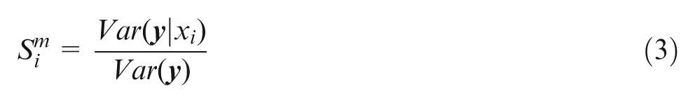
The main effect reflects the portion of scatter of $y$ that is directly caused by the scatter of $x_{i}$ without respecting interactions between $x_{i}$ and other input parameters.

In contrast, the total effect of the respective input $S_{i}^{t}$ also takes interactions between the considered input parameter $x_{i}$ and other input parameters $x_{j}, j = 1, \dots, i - 1, i + 1, \dots, N$ , into account. It can be computed by

S_{i}^{t} = \frac{Var (y | x_{i})}{Var (y)} + \sum_{j} \frac{Var (y | x_{i}, x_{j})}{Var (y)}

(4)

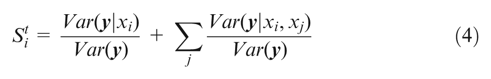
Thus, the total effect can be understood as the total influence the scatter of $x_{i}$ has on the scatter of $y$ .

The results of the sensitivity analysis are in general the more precise the more calculations of the functional relationship are performed.³⁰ Since the evaluation of the structural response via the FE method is quite computational demanding, it is advisable to employ a meta-model which reflects the underlying relationship approximately. Thereby, the functional relationship f(X) can be evaluated considerably faster. For this purpose, for example, again different methods like neural networks or decision trees can be used. The selection of an adequate meta-model can, for example, be performed on the basis of the coefficient of prognosis,³¹ which can be interpreted as a generalization of the coefficient of determination $R^{2}$ known from regression analysis. However, in the context of structural performance, the response surface method is a widely applied meta-modelling technique.^32–34

Analysis of robustness

A manufacturing process is said to be robust if the fluctuation of the response exceeds the fluctuation of the input parameters only little.³⁵ Robust processes are hence desirable because it is supposed that fluctuations of the response can be reduced by reducing the fluctuation of the inputs. If a process is not robust, this is not possible because the response obviously underlies fluctuations, which cannot be explained by the input fluctuations. The definition of a robust process can be translated to a product. Such is a product or design robust, if the behaviour and the performance can easily be predicted under varying input and ambient parameters.³⁶ A straightforward approach for the evaluation of robustness is the computation and the comparison of the coefficient of variation $CV$

CV = \frac{σ}{μ} = \frac{sample standard deviation}{sample mean}

(5)

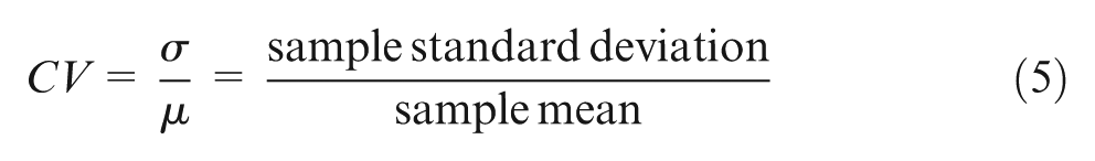
First, the $CV$ of every input parameter is computed and thereafter compared with the $CV$ of the response. If the $CV$ of the response is clearly larger than the largest input $CV$ , then the process (or the product) is said to be non-robust. Otherwise, the converse is true.³⁵

Analysis of reliability

In the context of structural performance evaluation, the probability of failure can be defined as the probability that the response of the structure exceeds the limit state. This limit state is the specific limit, for when exceeding it, the structure is unable to perform as required.²⁵ In the following, we focus on the maximum deformation as an indicator for the structural performance.

Assuming a Gaussian distribution for the maximum deformation, the probability of failure, that is the probability that the maximum deformation d exceeds the given limit state $d_{crit}$ , can be determined with estimated values for the mean $\hat{μ}$ and standard deviation $\hat{σ}$ by (see Figure 2)

P (d > d_{crit}) = 1 - F_{N (\hat{μ}, \hat{σ})} (d = d_{crit})

(6)

where $F_{N (\hat{μ}, \hat{σ})} (\cdot)$ is the cumulative distribution function of the Gaussian distribution with mean $\hat{μ}$ and standard deviation $\hat{σ}$ .

Figure 2.

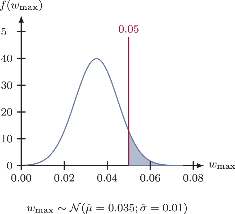
Probability of failure from an estimated Gaussian distribution.

Of course, the assumption of a Gaussian distribution for the maximum deformation is not always tenable. In such cases, models for higher moments of the samples can be estimated and employed to describe the expected distribution of the maximum deformation. However, even then the respective formulation of equation (6) is still applicable.

Determining the effects of geometric deviations on the structural performance

Since the introduced approaches for the probabilistic analysis of structural performance explained before seem imperfect for certain applications, another procedure is proposed. For this purpose, first a central composite design (CCD) plan is formed with parametric variations of the geometry as can be seen from Figure 3(a). It should be mentioned that also other kinds of experimental design plans could have been employed like sampling plans as, for example, based on the latin hypercube sampling. However, the CCD plan offers advantages when applying the response surface methodology with quadratic regression models.³⁷ However, each row of the experimental design plan contains a geometric variant of the part. For each of these geometric variants, multiple FE runs are performed, where fluctuating material properties and geometric deviations are taken into account (see Figure 3(b)). Both fluctuating material properties and geometric deviations are modelled by random fields. This means that geometric variants of the part are generated via the CCD plan and geometric deviations of form and shape are created by employing a random field approach. Therefore, this proceeding enhances the straight parametric approach for the consideration of geometric deviations with the random field method.

Figure 3.

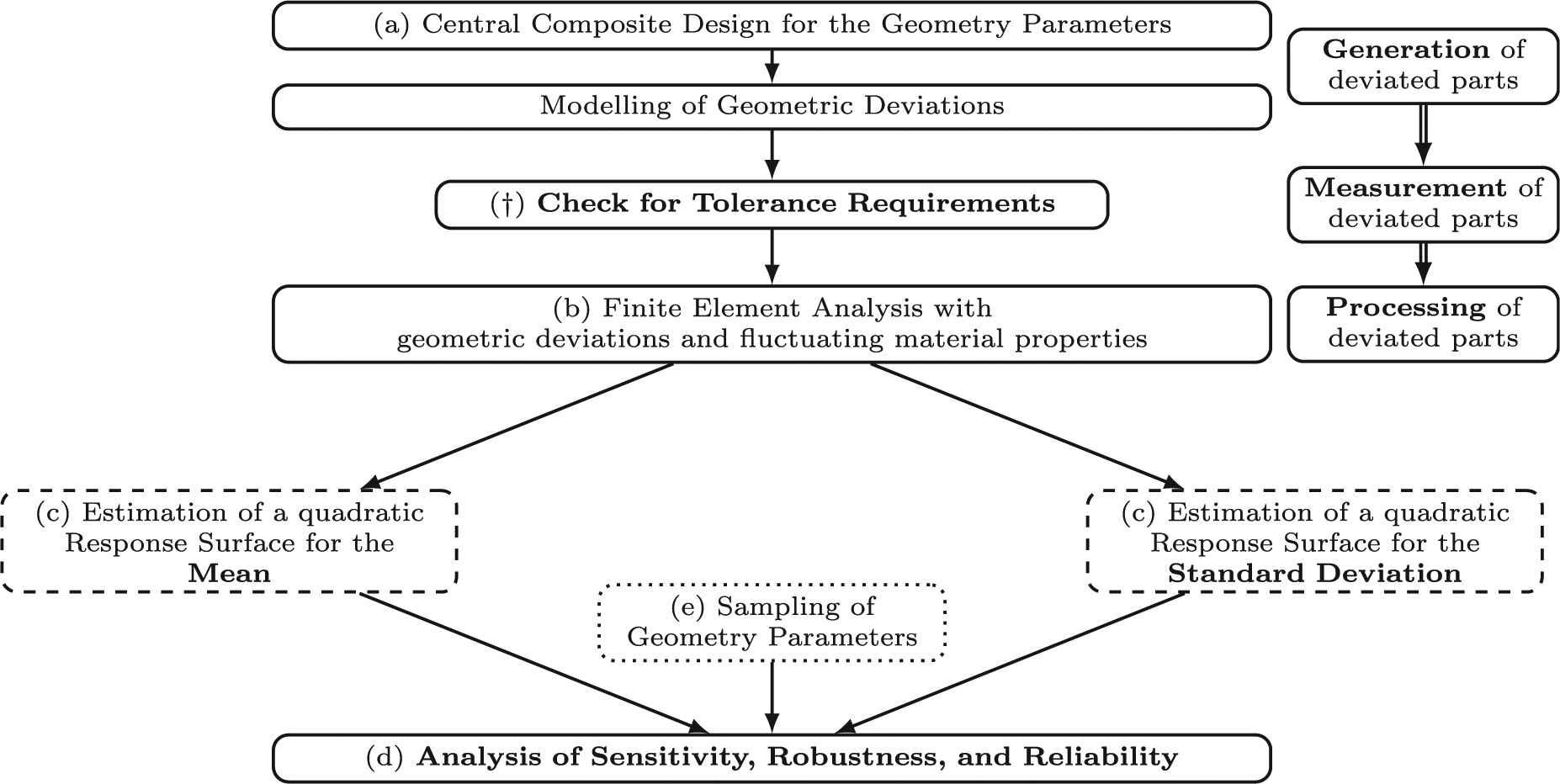
Approach for the determination of the effects of geometric deviations on the structural performance.

The results of the FE runs for each geometric variant are then used to estimate a quadratic response surface model for the mean and the standard deviation of the maximum deformation (see Figure 3(c)). These models can then be used for the analysis of sensitivity (the evaluation of main contributors to the response), the analysis of robustness and the evaluation of reliability (see Figure 3(d)). For the sensitivity analysis as well as for the evaluation of reliability, sampling methods may be used for creating random (in contrast to the CCD plan) geometric variants (see Figure 3(e)). For each of these random variants, the mean and the standard deviation of the maximum deformation can be estimated by the respective response surface models. Assuming a Gaussian distribution for the maximum deformation, it is hence possible to determine the probability of failure based on these values. The estimated regression models can also be used to determine the effect of the geometry parameters on the so-calculated probability of failure.

Since this approach is based on the modelling of geometric deviations instead of employing a particular model for the representation of geometric tolerances, also the effects of different tolerance requirements on the structural performance can easily be analysed. For this purpose, a digital check for tolerance requirements has to be performed previously to the FE runs (see Figure 3(†)). This means that every generated deviated part is virtually measured with regard to the tolerance requirements to be analysed and that only the deformation data of parts which fulfil the tolerance requirements are taken into account in the estimation of the response surfaces. In doing so, the effects of geometric tolerances on the structural performance and especially on the probability of failure can be investigated, which can be of great benefit in manners of tolerance analysis activities. It is worth mentioning that this approach is not limited to a specific tolerancing standard or tolerance representation scheme since geometric deviations are modelled instead of geometric tolerances. It therefore allows the consideration of any 2D or 3D tolerances in tolerance analysis. In summary, the proposed approach reflects the reality in this sense that deviated parts are generated, measured and processed digitally. Based on the obtained results, limits for the allowable geometric deviations in terms of 2D or 3D geometric tolerances can be set more easily.

Case study

The proposed approach is now applied to a simple case study where geometric deviations of form and shape as well as fluctuating material properties are taken into account in the structural performance evaluation.

Introduction, design plan, and parameter settings

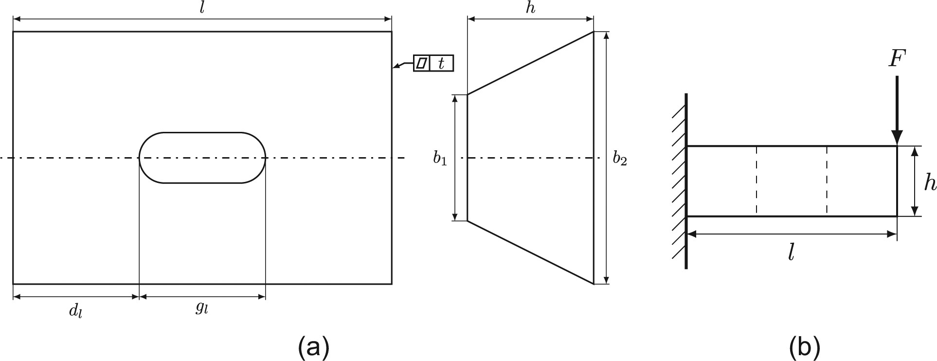
The reference part for this case study is a cantilever beam in bending as illustrated in Figure 4. The geometry parameters are the height h, the length l, the lower width $b_{1}$ , the upper width $b_{2}$ , the distance of the long hole from the fixation d_l and the length of the long hole $g_{l}$ . The beam is fixated on one side and stressed by a force on the other side. The measures are $h = 10 mm, l = 30 mm, b_{1} = 10 mm, b_{2} = 20 mm, d_{l} = 10 mm$ and g_l = 10 mm, the force is $F = 1000 N$ .

Figure 4.

Reference part of the case study.

As described above, first, a CCD plan is formed based on these parameters. Based on this plan, for each geometric variant, a deterministic finite element analysis (FEA) and multiple FE runs where random geometric deviations and fluctuating material properties are taken into account are performed.

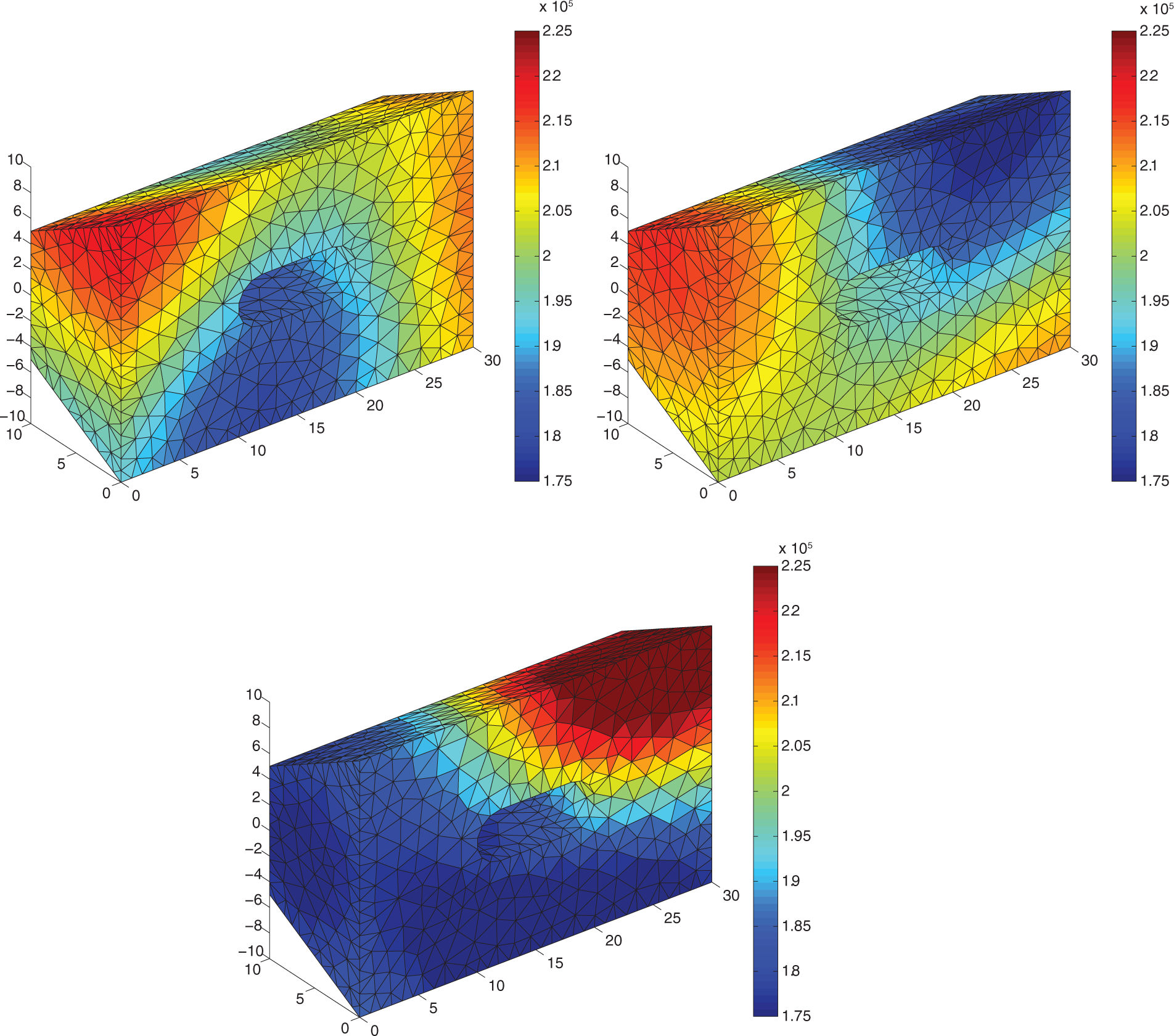
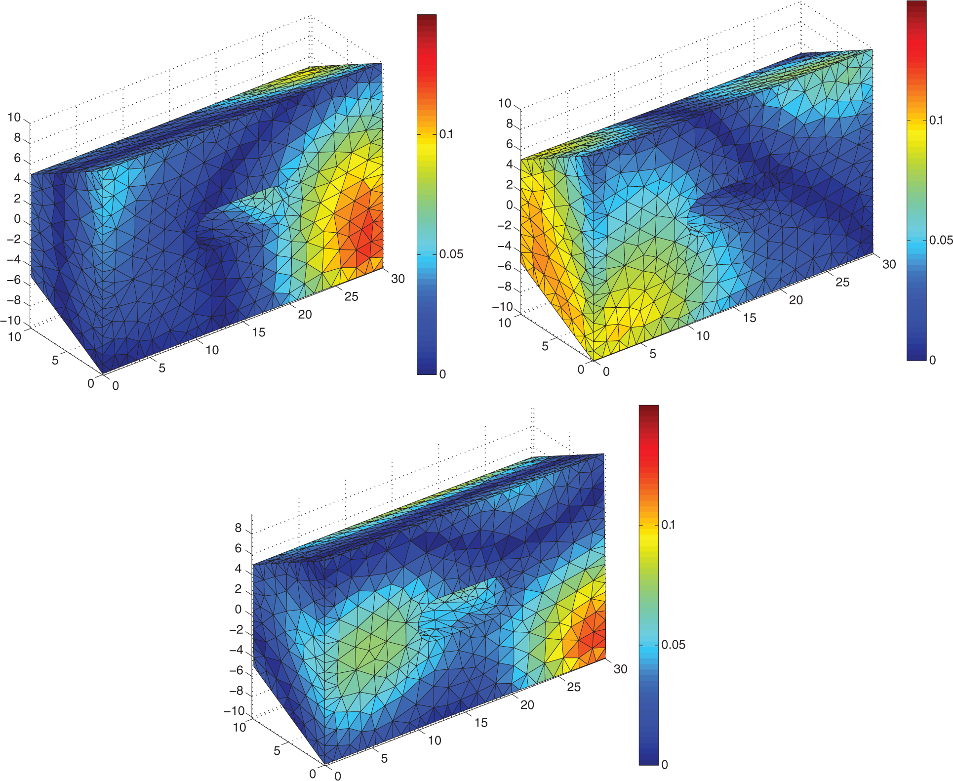
For modelling geometric deviations, a Gaussian random field approach is used to deviate the tetrahedral mesh nodes within 3D space. The correlation length of the squared exponential correlation function is set to $l_{ρ}^{geom} = 15 mm$ , the standard deviation to σ^geom = 0.1 mm and the mean to $μ^{geom} = 0$ . Three samples of the beam with deviated geometry are shown in Figure 5, where the colours indicate the geometric deviation compared to the nominal geometry.

Figure 5.

Three samples of the beam in bending with geometric deviations of form and shape.

Furthermore, we assume that the material properties of the beam in bending can also be described by a Gaussian random field. The mean of the Young’s modulus is assumed to be $μ^{mat} = 200, 000 N / m m^{2}$ , the standard deviation $σ^{mat} = 20, 000 N / m m^{2}$ and the correlation length of a squared exponential correlation function $l_{ρ}^{mat} = 15 mm$ . We use the midpoint method to discretize the random field.³⁸ Following that, the Young’s modulus of each element can be approximated by the value of the random field at the element’s centroid. Figure 6 shows three samples of the beam in bending where the colours illustrate the value of the element’s Young’s modulus.

Figure 6.

Three samples of the beam in bending with fluctuating material properties (Young’s modulus).

Overall, for each variant in the CCD plan, a deterministic FEA and 100 runs of a FE analysis with fluctuating material properties and geometric deviations are performed. Based on these data, the mean and standard deviation of the maximum deformation for each variant can be computed. From this, a (quadratic) response surface for the mean as well as for the standard deviation can be estimated. The coefficient of determination for the mean response surface is R² = 99.98% and R² = 97.29% for the standard deviation response surface. Hence, the underlying quadratic models seem to be good estimates of the true relationship between the geometry parameters and the mean and standard deviation of the maximum deformation of the beam within the given geometry parameter intervals.

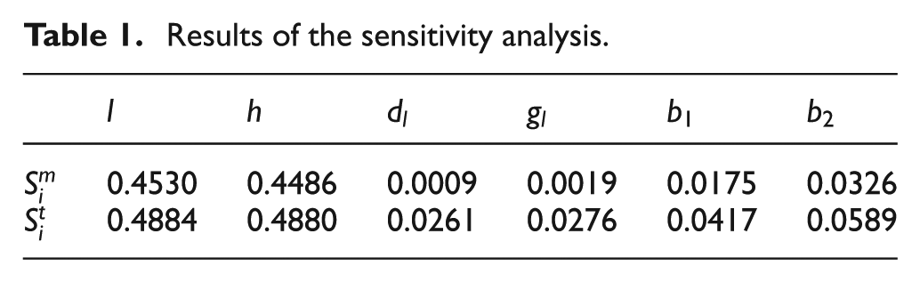
The sensitivity analysis can then be performed based on the estimated mean model. The results for the main and total effects of the geometry parameters are given in Table 1.

Table 1.

Results of the sensitivity analysis

	$l$	$h$	$d_{l}$	$g_{l}$	$b_{1}$	$b_{2}$
$S_{i}^{m}$	0.4530	0.4486	0.0009	0.0019	0.0175	0.0326
$S_{i}^{t}$	0.4884	0.4880	0.0261	0.0276	0.0417	0.0589

In this example, the coefficient of variation is 5.37% for every input parameter, since the variation of the input parameters is given by the CCD plan. The coefficient of variation of the maximum deformation is 20.24% for the deterministic FEA and 21.75% when taking geometric deviations of form and shape as well as fluctuating material properties into account.

The limit for the maximum deformation may be given to $d_{crit} = 0.05 mm$ , and the distribution laws for the input geometry parameters are assumed to be $h ~ N (10, 0.3), l ~ N (30, 1), b_{1} ~ N (10, 0.3), b_{2} ~ N (20, 0.65)$ . The mean probability of failure of these sample combinations taking fluctuations of the material properties and geometric deviations into account is 17.43%. In contrast to that, the mean probability of failure estimated from the deterministic FEA involving only parametric geometric deviations is 13.25%.

The effects of form tolerances on the probability of failure

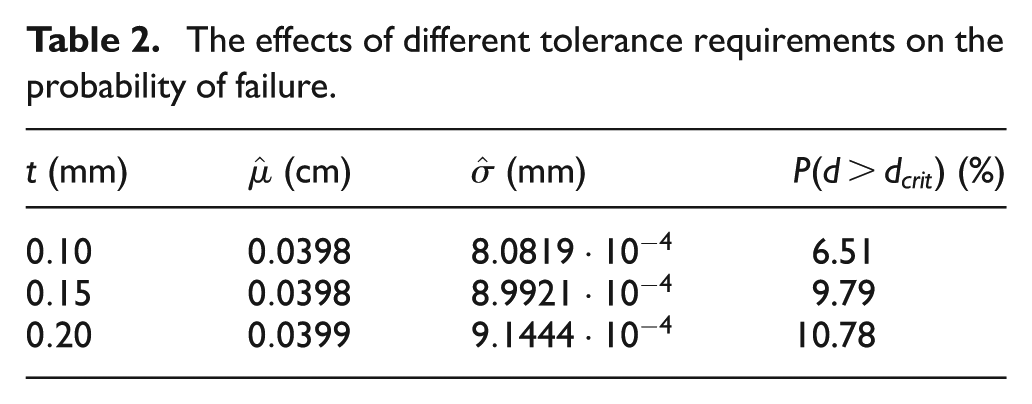
The evaluation of the effects of form tolerances on the structural performance may also be highlighted in a simple example. Given again the beam shown in Figure 4 with the nominal measures and a flatness tolerance of size t on the front plane. We now want to determine the effects of t on the probability of failure, in this case, the probability that the maximum deformation exceeds the limit of $d_{crit} = 0.041 mm$ .

In order to perform this, the procedure explained before is employed. That means that several FE runs are performed where geometric deviations modelled by random fields are taken into account. For this sub-example, we vary the standard deviation of the random field between $σ^{geom} = (0.1 mm; 0.15 mm; 0.2 mm)$ . The values for the mean and the correlation length of the random field stay at μ^geom and $l_{ρ}^{geom} = 15 mm$ , respectively. Note that since we are only interested in the effects of geometric deviations, no fluctuations of the material properties are taken into account, and therefore, the Young’s modulus is set to $μ^{mat} = 200, 000 N / m m^{2}$ for every element. For each generated geometry, we measure the flatness tolerance of the front plane. We then compare these values with the given tolerance requirement that we want to analyse. Only those geometries are then taken into account for the estimation of the response surfaces that fulfil these relevant tolerance requirements. Table 2 shows the effects of the flatness tolerance limit t for the front plane of the beam on the estimated mean $\hat{μ}$ and estimated standard deviation $\hat{σ}$ of the maximum deformation and the probability of failure $P (d > d_{crit})$ .

Table 2.

The effects of different tolerance requirements on the probability of failure

$t$ (mm)	$\hat{μ}$ (cm)	$\hat{σ}$ (mm)	$P (d > d_{crit})$ (%)
$0.10$	$0.0398$	8.0819 · 10⁻⁴	6.51
$0.15$	$0.0398$	$8.9921 \cdot 10^{- 4}$	9.79
$0.20$	0.0399	$9.1444 \cdot 10^{- 4}$	10.78

Summary of the results

It can be seen that the consideration of geometric deviations and fluctuating material properties can lead to a better understanding and a more precise image of the behaviour of a part within a FE analysis. The results show that the main contributors to the maximum deformation of the beam are the length l and the height h. Furthermore, the deterministic FEA overrates the robustness of the design and underestimates the probability of failure. The results are illustrated in Figure 7.

Figure 7.

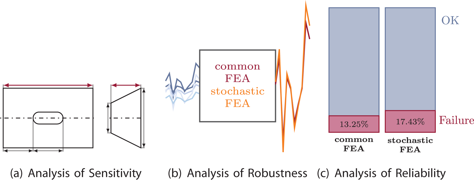
Results of the case study.

In addition, the value of the flatness tolerance zone has obviously an effect on the probability of failure. In order to assure a probability of failure less than 10%, a flatness tolerance of $t = 0.15$ for the front plane seems thus adequate (see Table 2). Based on these results, the product developer is enabled to optimize the product design parameters considering the structural performance as well as to deduce 3D tolerances such as tolerances of form, orientation, location and run-out.

Conclusion and outlook

The impact of geometric deviations on the structural performance is of high interest in the context of computer-aided tolerancing. Therefore, this article proposes an approach which makes use of the functionalities of modern parametric CAD systems and enhances them by taking fluctuating material properties and geometric deviations into account. For this purpose, a CCD plan is linked to a non-intrusive stochastic FE approach employing random fields to describe material fluctuations and geometric deviations. Moreover, regression analysis and methods of sensitivity analysis and analysis of robustness are used to identify the main geometric contributors, to evaluate the robustness of the design and to predict the probability of failure.

The main goal is to draw an image of the part’s behaviour that is close to reality and enables the product developer to predict possible issues and design imperfections. Questions about the main geometric contributors to the structural performance and about the robustness and the reliability of the design can be answered more precisely. Furthermore, the effects of form and position tolerances on the probability of failure can also be predicted. These results can then be used in the context of computer-aided tolerancing for setting optimal tolerance requirements.

However, the improvement of this approach with respect to the computational effort as well as the integration of the obtained results in adequate models for the representation of geometric tolerances and in tolerance analysis remain future research directions.

Footnotes

Funding

This research received no specific grant from any funding agency in the public, commercial or not-for-profit sectors.

References

Zhang

Anwer

Mathieu

. A discrete geometry framework for geometrical product specifications. In: CIRP design conference, 2011. Proceedings of the 21st CIRP Design Conference, KAIST, Daejeon (South Korea), pp.142–148, March 2011.

Armillotta

Semeraro

. Geometric tolerance specification. In: Colosimo

Senin

(eds) Geometric tolerances – impact on product design, quality inspection and statistical process monitoring. London: Springer-Verlag, 2011, pp. 3–37.

Mathieu

Ballu

. A model for a coherent and complete tolerancing process. In: Davidson

(ed.) Models for computer aided tolerancing in design and manufacturing. Netherlands: Springer, 2007, pp.35–44.

Dantan

Ballu

Mathieu

. Geometrical product specification – model for product life cycle. Comput Aided Design 2008; 40: 493–501.

Desrochers

Clément

. A dimensioning and tolerancing assistance model for CAD/CAM systems. Int J Adv Manuf Tech 1994; 9: 352–361.

Chase

Magleby

Gao

. Tolerance analysis of 2-D and 3-D mechanical assemblies with small kinematic adjustments. In: Zhang

Hong-Chao

(ed.) Advanced tolerancing techniques. New York: John Wiley & Sons Ltd, 1997, pp.103–138.

Giordano

Samper

Petit

. Tolerance analysis and synthesis by means of deviation domains, axi-symmetric cases. In: Davidson

(ed.) Models for computer aided tolerancing in design and manufacturing. Netherlands: Springer, 2007, pp.85–94.

Hong

Chang

. A comprehensive review of tolerancing research. Int J Prod Res 2002; 40(11): 2425–2459.

Charpentier

Ballu

Pailhes

. A scientific point of view of a simple industrial tolerancing process. In: Proceedings of the 12th CIRP conference on computer aided tolerancing, Hudderseld, UK, April 2012.

10.

Zhao

Pasupathy

TMK

Wilhelm

. Modeling and representation of geometric tolerances information in integrated measurement processes. Comput Ind 2006; 57: 319–330.

11.

Baysal

Roy

Sudarsan

. The open assembly model for the exchange of assembly and tolerance information: overview and example. In: Proceedings of the 2004 ASME international design engineering technical conferences & computers and information in engineering conference, September 28–October 2, 2004, Salt Lake City, Utah, USA.

12.

Zhang

Tang

. An integrated modeling method of unified tolerance representation for mechanical product. Int J Adv Manuf Tech 2010; 46: 217–226.

13.

Samper

Giordano

. Taking into account elastic displacements in 3D tolerancing models and application. J Mater Process Tech 1998; 78: 156–162.

14.

Lustig

Hochmuth

Meerkamm

. Enhancement in coupling tolerance analysis and elastic deformations on the example of a linear support system. In: Proceedings of the 15th international conference on engineering design (ICED05), 2005, August, Melbourne, Australia.

15.

Stockinger

Lustig

Meerkamm

. Computer-based and experimental validation of an approach to combine tolerance zones with elastic deformations. In: Proceedings of the 16th international conference on engineering design (ICED07), 2007 August, Paris, France.

16.

Walter

Wartzack

. Analysis of the effects of manufacturing-caused deviations and varying operation parameters on operation-depending deviations of systems in motion. In: Proceedings of the 12th CIRP conference on computer aided tolerancing, Huddersfield, UK, April 2012.

17.

DIN EN ISO 17450–1:2009. Geometrische Produktspezifikation (GPS) – Grundlagen.

18.

Zhang

. Discrete shape modeling for geometrical product specifications: contributions and applications to skin model simulation. Ecole Normale Superieure de Cachan, 2011 Laboratoire Universitaire de Recherche en Production Automatisee, 61, avenue du President Wilson - Cachan cedex, France.

19.

Henke

Summerhays

Baldwin

. Methods for evaluation of systematic geometric deviations in machined parts and their relationships to process variables. Precis Eng 1999; 23(4): 273–292.

20.

Desta

Feng

Ouyang

. Characterization of general systematic form errors for circular features. 2002. International Journal of Machine Tools and Manufacture, Volume 43, Issue 11, September 2003, pp. 1069–1078.

21.

Vajna

Weber

Bley

. CAx für Ingenieure. Berlin/Heidelberg: Springer-Verlag, 2009.

22.

Stoll

. Generieren von nichtidealer Geometrie. In: 17th symposium‘Design for X’, 2006. Proceedings of the 17. Symposium “Design for X”, Neukirchen, Germany, 2006, October.

23.

Stoll

Wittmann

Meerkamm

. Tolerance analysis with detailed part modeling In: Giordano

Mathieu

Villeneuve

: Product Life-Cycle Management. Geometric Variations. London: ISTE Ltd., John Whiley Sons Inc., 2010 ISBN: 9781848212763.

24.

Bayer

Einzinger

Roos

. Random fields: theory and applications. In: Proceedings of the Weimarer optimization and stochastic days 6.0, Weimar, Germany, October 2009.

25.

Choi

Grandhi

Canfield

. Reliability-based structural design. London: Springer-Verlag, 2007.

26.

Bucher

. Computational analysis of randomness in structural mechanics. London: Taylor & Francis Group, 2009.

27.

Alberty

Carstensen

Funken

. Matlab implementation of the finite element method in elasticity. Computing 2002; 69(3): 239–263.

28.

Qiu

KLH

Gao

Sun

. Comparison of stochastic response surface method and response surface method for structure reliability analysis. In: Lin

Qiu

Haobo

Gao

Liang

Sun

Yifei

;, “Comparison of Stochastic Response Surface Method and Response Surface Method for Structure Reliability Analysis,” Intelligent Computation Technology and Automation, 2009. ICI-CTA ’09. Second International Conference on, vol.3, no., pp.172–175, 10–11 Oct. 2009.

29.

Kewlani

Iagnemma

. A stochastic response surface approach to statistical prediction of mobile robot mobility. In: Intelligent Robots and Systems, 2008. IROS 2008. IEEE/RSJ International Conference on, 22–126 Sept. 2008, pp. 2234–2239.

30.

Saltelli

. Global sensitivity analysis: the primer. Chichester, England: John Wiley & Sons Ltd, 2008.

31.

Most

Will

. Meta-model of optimal prognosis – an automatic approach for variable reduction and optimal meta-model selection. In: Proceedings of the Weimarer optimization and stochastic days 5.0, 2008, Weimar, Germany, November 2008.

32.

Myers

Montgomery

Anderson-Cook

. Response surface methodology – process and product optimization using designed experiments. Hoboken, NJ: John Wiley & Sons Ltd, 2009.

33.

Wie

Cui

Chen

. Optimization and tolerance prediction of sheet metal forming process using response surface model. Comp Mater Sci 2008; 42: 228–233.

34.

Kleiber

Knabel

Rojek

. Response surface method for probabilistic assessment of metal forming failures. Int J Numer Meth Eng 2004; 60: 51–67.

35.

Reuter

Hülsmann

. Achieving design targets through stochastic simulation. In: MADYMO users’ conference, 2000, Paris, May 2000.

36.

Reh

Beley

Mukherjee

. Design for six sigma und robust design. In: Proceedings of the Weimarer optimization and stochastic days 2.0, 2005, Weimar, Germany, December 2005.

37.

Siebertz

Van Bebber

Hochkirchen

. Statistische Versuchsplanung. Berlin/Heidelberg: Springer-Verlag, 2010.

38.

Sudret

Kiureghian

. Stochastic finite element methods and reliability. UCB/SEMM-2000/08, 2000. Berkeley, CA: Department of Civil & Environmental Engineering, University of California, November 2000.

How to determine the influence of geometric deviations on elastic deformations and the structural performance?

Abstract

Keywords

Structural performance evaluation in computer-aided tolerancing

Modelling geometric deviations

Evaluation of the structural performance

The FE method

Probabilistic approaches for the evaluation of structural performance

Intrusive approaches

Non-intrusive approaches

Analysis of sensitivity

Analysis of robustness

Analysis of reliability

Determining the effects of geometric deviations on the structural performance

Case study

Introduction, design plan, and parameter settings

The effects of form tolerances on the probability of failure

Summary of the results

Conclusion and outlook

Footnotes

Funding

References