
Abstract
A novel approach is proposed for the characterization of critical dimensions and geometric errors, suitable for application to micro-fabricated parts and devices characterized as step-like structured surfaces. The approach is based on acquiring areal maps with a high-precision optical three-dimensional profilometer and on processing topography data with novel techniques obtained by merging knowledge and algorithms from surface metrology, dimensional metrology and computer vision/image processing. Thin-foil laser targets for ion acceleration experiments are selected as the test subject. The main issues related to general applicability and metrological performance of the methodology are identified and discussed.
Introduction
Dimensional and geometric error verification of parts fabricated at micrometric and sub-micrometric scales is currently difficult. Scanning electron microscope (SEM) images provide the bulk of visualization capability but mostly provide only qualitative information; micro and nano precision coordinate measuring machines (CMMs), such as the Zeiss F25 1 or the IBS ISARA Ultra Precision CMM, 2 require long measuring times and skilled operators. Micro-fabricated parts are consequently subjected to high defect rates, and improving the manufacturing process is difficult without easily available quantitative data.
New solutions are increasingly being made commercially available for surface metrology at micro and sub-micrometric scales: 3 three-dimensional (3D) profilometers and microscopes capture quantitative surface topography information as areal maps, and – albeit they are primarily designed for surface finish assessment (e.g. through 3D field parameters, see ISO/FDIS 25178-2:2011 and related literature 4 ) – they can also be used to acquire geometric information of micro-fabricated parts.
The objective of this work is to propose a general approach to the evaluation of critical dimensions and geometric errors on micro parts and devices characterized by step-like structured surfaces, based on applying the principles of ISO 17450-1:2011 (Geometrical product specifications (GPS) – General concepts – Part 1: Model for geometrical specification and verification) to the analysis of areal maps obtained by optical 3D profilometers. The approach is based on merging ideas and procedures derived from surface metrology, dimensional metrology and also from computer vision/image processing, since the acquired areal maps are essentially range images, and can be handled as such in many steps of the analysis procedure.
The approach is validated through an example application involving the verification of thin-foil laser targets. These are micro-fabricated, prototype devices characterized by step-like structured surfaces, produced by the STFC (Science and Technology Facilities Council, UK) for use in ion acceleration experiments.
The proposed approach
Premise: optical 3D profilometers as range imaging devices
The proposed approach has its foundations in the use of commercial optical 3D profilometers for acquiring the 3D topography of the surfaces of the part or device subjected to verification.
The present work focuses in particular on instruments operating as 3D imaging devices, i.e. returning a matrix of height values, measured along the direction of observation z (also known as the vertical direction), and arranged onto a rectangular uniform grid on the xy acquisition plane (see the example in Figure 1). The result of the acquisition process is an areal map, or range image, where each height value is encoded into the equivalent of a pixel (Figure 1(b)). This is also referred to as a structured dataset, since the height values are arranged in an organized form (a matrix) and can be easily accessed through indices. The structured dataset intrinsically embeds point connectivity/neighbouring information, since adjacent points can be retrieved through sequential indices. The range image can be handled as an intensity (i.e. greyscale) image, meaning that a wide array of existing image processing algorithms can be applied; and/or it can be converted to a set of sparse x,y,z points (Figure 1(c)), which is typically referred to as an unstructured dataset because the gridded structure is lost, and so is connectivity information (albeit it should be noted that through pixel labelling, a parallel connectivity graph could be retained before converting the range image to sparse points). The conversion from range image to sparse points is possible because the calibrated instrument also returns pixel size/spacing in the xy plane. Notice that pixels are not necessarily square, as x and y spacing may differ (depending on the instrument camera); moreover, any distortion in the grid is assumed as corrected by calibration.
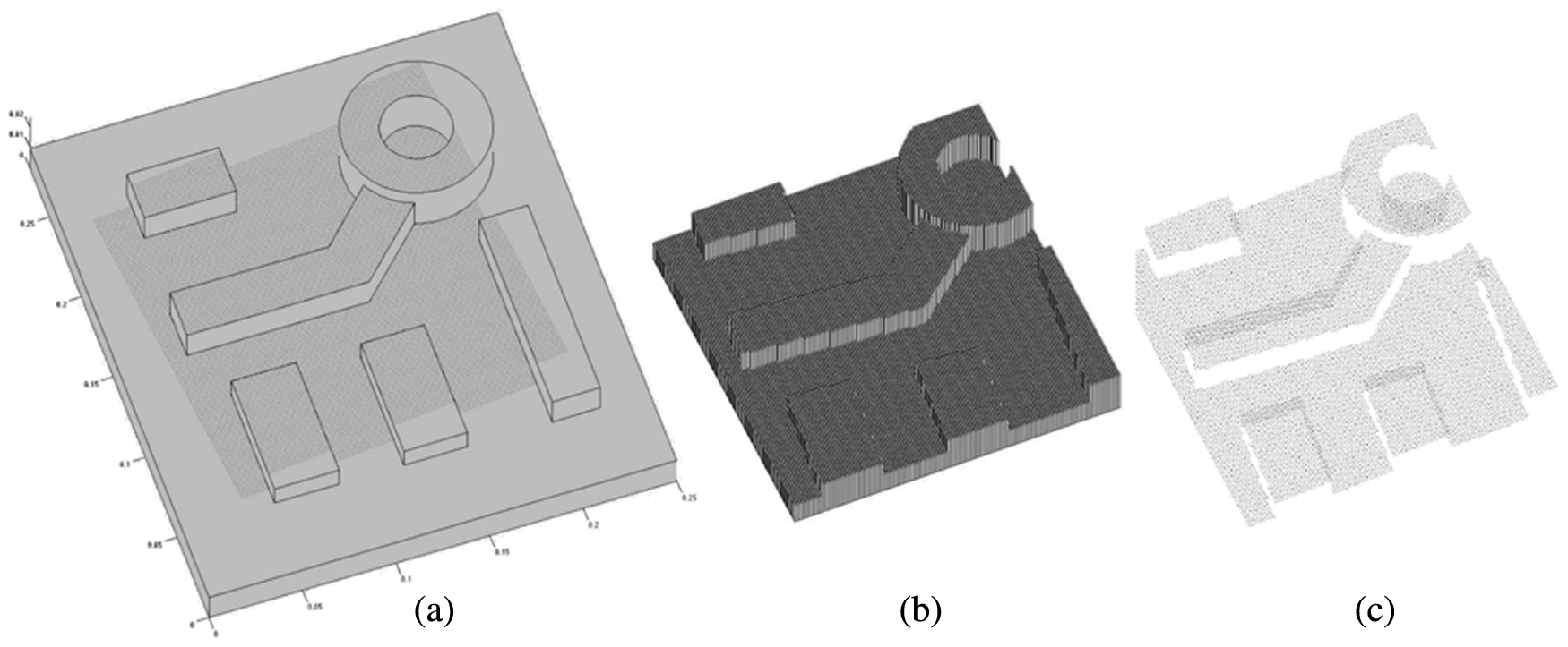
Acquisition of an example step-like structured surface: (a) acquisition area on the measurand surface; (b) range image; (c) sparse point set.
Optical 3D profilometers based on vertical scanning interferometry (VSI), and in particular white light scanning interferometry (WLSI) are selected as the instrument class of reference, albeit most of the considerations in the following also apply to optical profilometers based on dynamic-focus probes, and may be extended to include also single-point measurement devices, as long as they implement a raster scanning strategy over the measurand topography (so that the final output can still be considered a range image).
Step 1: measurement process planning and execution
The first step of the proposed approach consists of setting up the process parameters for acquiring the topography of the measurand with the optical 3D profilometer; this implies considering several important aspects, as illustrated in the following.
Range-imaging issues
By referring again to Figure 1, a number of issues are immediately evident:
- measurand coverage may be sub-optimal, given the rectangular acquisition area;
- uniform sampling density may be sub-optimal, if compared with feature-based density;
- unidirectional observation may lead to shadowed regions, particularly on samples tilted with respect to the measurement plane.
It should be noted that the above issues may be at least partially dealt with by stitching multiple datasets acquired with different orientations and sampling densities. However, stitching is still the subject of critical research,5,6 as registration of multiple datasets leads to the introduction of additional sources of error, and therefore is not considered in this work, which assumes a single range image is available at measurement.
Imaging resolution and range
Another typical issue related to imaging is ensuring that the metrological performance of the optical instrument is compatible with the verification task. In particular the vertical (z) and lateral (x,y) range and resolution of the optical profilometer must allow for an acceptable sampling of the measurand geometry.
For example white light scanning interferometry (WLSI) instruments can achieve working vertical resolutions < 0.1 nm, which is generally more than adequate for most micro-parts and devices, while simultaneously providing vertical ranges up to 100 μm, which may be suitable for a wide array of micro-fabricated products, but may not be compatible with very high aspect-ratio specimens.
For WLSI instruments, a working lateral resolution and range are derived from the combined properties of the camera charge-coupled device (CCD) and of the objective lens. High lateral resolutions, which are needed to guarantee an adequate sampling density according to the Nyquist criterion, can be achieved by means of high magnification objectives; high magnifications (and thus, high numerical apertures) this in turn allows the achievement of higher optical resolutions according to the Rayleigh criterion, which means a smaller minimum distance between two lateral features on a surface that can be distinguished (a 50× magnification typically leads to approximately 0.5 μm optical resolution). For a WLSI instrument with a 50× and 1024 × 1024 CCD, optical resolution prevails over the lateral sampling resolution, meaning that pixels are smaller than the minimum resolvable distance. 7 This has important metrological implications, in particular when counting pixels to compute linear sizes and distances, because adjacent pixels may not contain independent measurements. Another important issue of high magnification is the decrease of lateral range, and the consequent reduction of areal coverage, which may be a problem for the metrological verification of comparatively larger specimens.
Maximum detectable slope
The maximum detectable slope for a WLSI instrument is again dependent on optical magnification, 7 and can reach up to about 30° with a 50× objective in commercial instruments (e.g. see Taylor Hobson 8 ), which means that high-slope surfaces (in addition to vertical walls) cannot be acquired in the default orientation of the specimen within the instrument working area. Tilting the specimen is often not an option since it is necessary to keep the measurand surface within the vertical range of the probe. This is definitely a relevant issue in the metrological verification of step-like structured surfaces.
Measurement uncertainty
Finally, measurement uncertainty information should be available to assess the ultimate meaningfulness and reliability of the results of quantitative inspection. However, this type of information is already hard to obtain for conventional imaging devices involved in surface metrology tasks,9–12 and even more so for range imaging devices such as optical 3D profilometers.
The geometric verification process
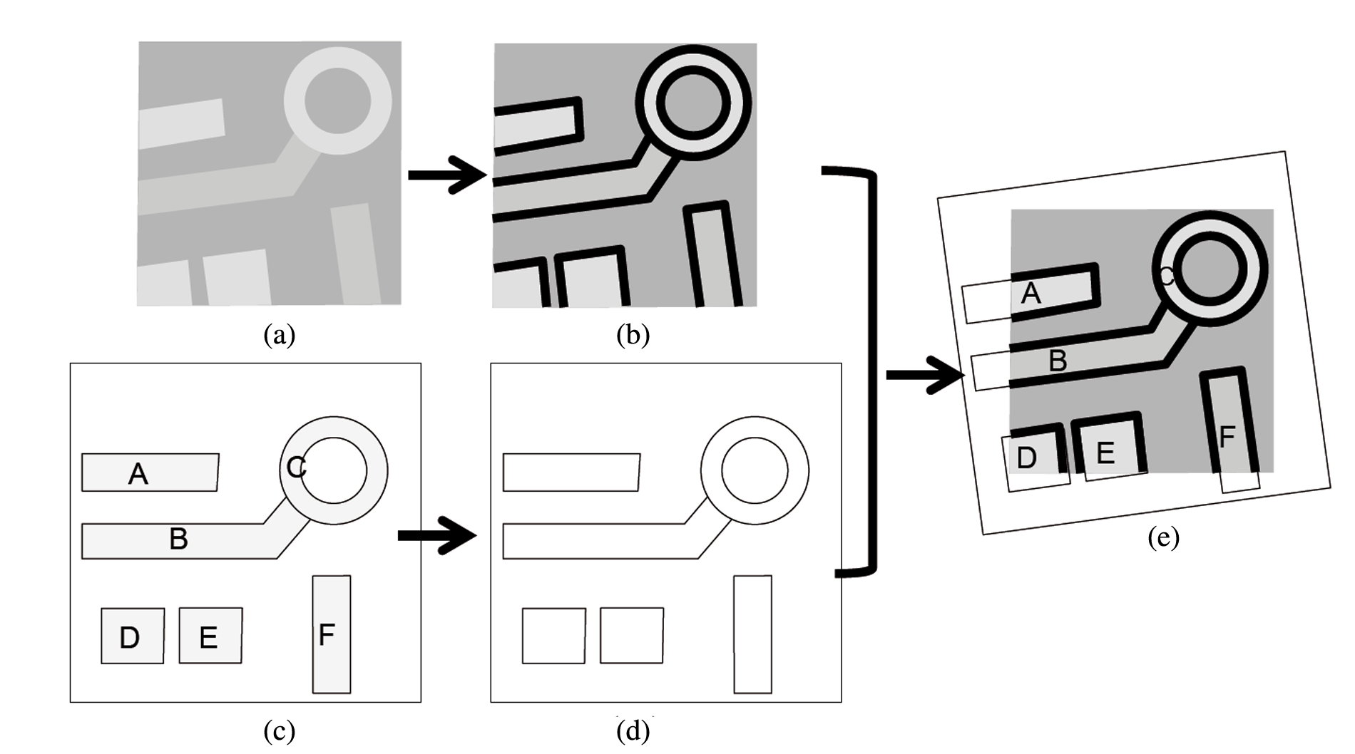
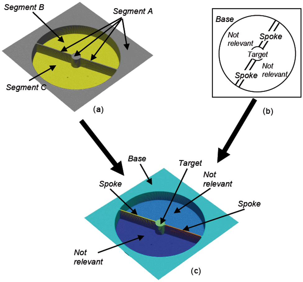
The proposed approach to the geometric verification process follows the workflow identified by ISO 17450-1, with the necessary adaptations to operate with unidirectional observation through a range imaging device, on a workpiece essentially defined by a structured surface with step-like features. The overall scheme of the verification process is summarized in Figure 2 and described in the following text.
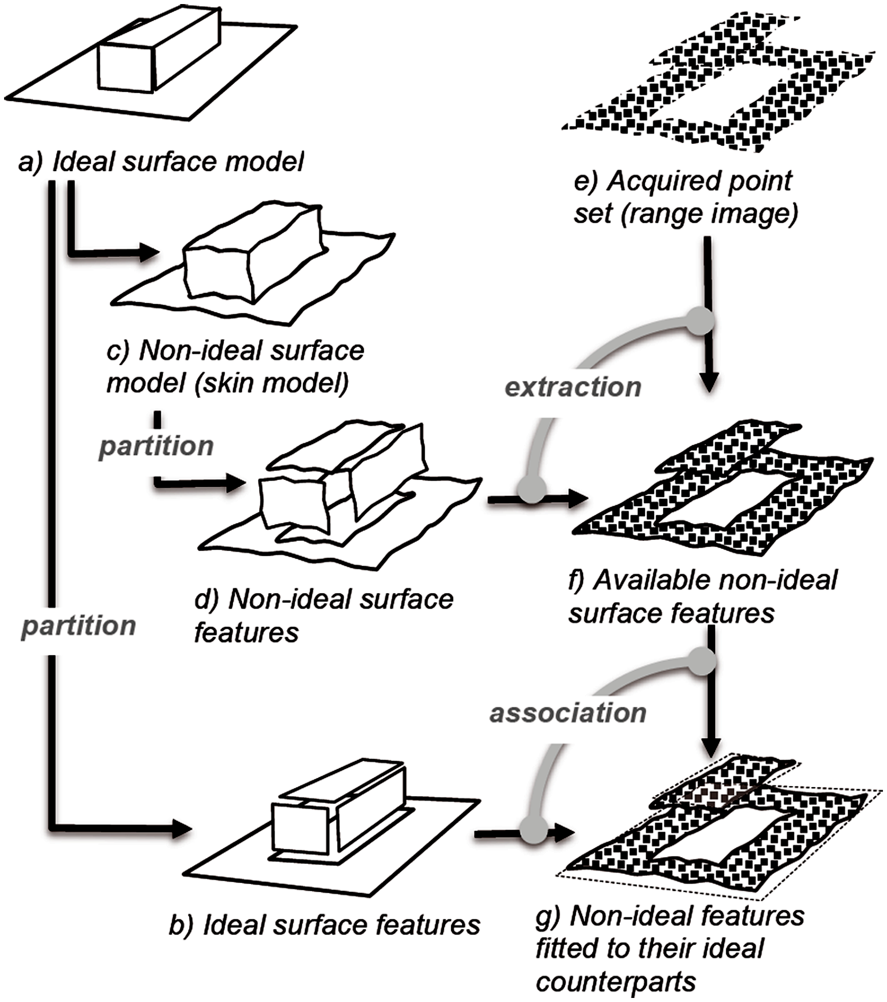
The process of geometric verification of a micro-part or device, according to ISO 17450-1, assuming a step-like structured surface acquired by means of a range imaging instrument.
An ideal surface model (ISO 17450-1 terminology) of the micro part or device must be available, preferably as CAD data (e.g. Figure 2(a)), decomposed through partition into ideal geometric features (points, lines and surfaces, e.g. Figure 2(b)), in turn defined by intrinsic characteristics (e.g. dimensions) and situation characteristics (relative position and orientation). Characteristics are assumed as potentially associated to specifications by dimensions and specification by zones (i.e. dimensional and geometric tolerances), albeit it is quite common for micro parts and devices not to be fully toleranced 13 (specifications are not shown in the models in Figure 2(a) and Figure 2(b)).
ISO 17450-1 introduces the additional concept of a non-ideal surface model (also known as skin model): essentially a container that gathers knowledge and expectations of the real geometry and how it varies with respect to the ideal one (Figure 2(c)). The skin model is decomposed into a set of non-ideal geometric features (Figure 2(d)), which generally replicates the organization of the ideal model. The skin model provides a convenient way of structuring workpiece-related information in an organized per-feature fashion.
Since this work is based on measurement data collected through a single imaging operation under unidirectional observation, the procedure assumes the availability of a single dataset, represented as a range image or unstructured point set depending on convenience (Figure 2(e)). Through extraction, portions of this point set are used to populate some of the non-ideal geometric features defined in the skin model (Figure 2(f)). Notice that, in general, only those non-ideal surface features that do not exceed the maximum detectable slope with respect to the direction of observation can be populated through extraction, which leaves out. in particular, vertical walls and undercuts. Thus, the verification process must be designed to consider such limitations. For each non-ideal surface feature for which data is available, verification takes place by association, which consists of fitting the non-ideal feature to its ideal counterpart (Figure 2(g)): from the fitting result, geometric deviations can be evaluated to assess whether the workpiece conforms to the specifications.
Step 2: raw data preprocessing
Preprocessing has the primary aim of “cleaning” the raw data acquired from the measurement instrument for example from missing data, measurement artefacts and levelling errors, which are typical errors affecting optical 3D profilometers. In the proposed approach, at preprocessing the dataset is retained in its range image form. The whole process is summarized in Figure 3 in a simplified form, on an example two-dimensional (2D) cross-section profile of a step topography.
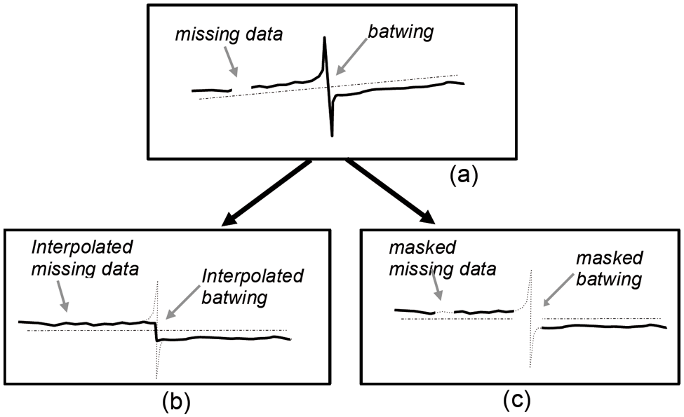
Preprocessing on an example, simplified 2D cross-section profile of a step topography: (a) missing data, batwing and levelling error in the raw data; (b) missing data and batwings replaced by median interpolation, levelling obtained by z-subtraction of the z-least-squares mean (z-LSM) plane; (c) missing data and artefacts voided by masking (the step may disappear), levelling obtained by z-subtraction of the z-LSM plane.
Missing data
Missing measurement values, referred to as missing data (see the example in Figure 3(a)), are given two alternative treatments: they can be replaced by interpolation from valid neighbours (Figure 3(b)), or they can be “voided” by appropriate image masking (Figure 3(c)). Interpolation is preferred as a temporary modification for facilitating segmentation and feature identification (see next step), but voiding by appropriate masking should be reintroduced before attempting any dimensional metrology task to avoid the influence of additional error sources owing to inaccurate assessment of height values.
For interpolating missing data, a median operator computed using valid values within a 3 × 3 moving window is used as the interpolant. The median is preferred over the arithmetic average since it better preserves step-like features (this is a given result from the image processing literature 14 ). Regions featuring multi-clustered missing data points can be handled by multiple interpolation iterations.
Measurement artefacts
These are measurement-process dependent and appear as false features (e.g. clustered topographic formations), usually in correspondence with specific measurand features. Typical measurement artefacts for vertical scanning interferometry (VSI) instruments are the “batwings”, which usually appear clustered in correspondence with step-like transitions on the measurand (see the example in Figure 3(a)). Different artefacts characterize other optical 3D profilometers. Unlike missing data, measurement artefacts must be identified before they can be treated. In the proposed approach a solution is applied, derived from a well known procedure for noise identification and removal in conventional image processing: batwings are recognized as outliers in the residual image obtained by subtracting the N × N median-filtered image from the original image (the size of the moving window is pre-emptively hardcoded based on the analysis of the interactions between the specific instrument–measurand pair). The approach works well under the assumption of regularity of the measurand, which is the case for structured step-like surfaces. It should be noted that many alternative approaches for removing measurement artefacts are possible, given the amount of literature available for noise removal in image processing. 14 Once identified, artefacts can undergo the usual two alternative treatments: either they are replaced by their interpolated counterpart (which is generally done for the next segmentation step, e.g. see Figure 3(b)), or they are marked as voids in the updated image mask to avoid error accumulation in dimensional metrology assessment (Figure 3(c)). Notice that voiding an artefact located in correspondence to a step may make it more difficult to identify the exact location of the step edge, which is undesirable if the step is connected to a relevant non-ideal feature (see the example in Figure 3(c)). In such cases, replacement by interpolation may be accepted for the actual verification process, even though it may introduce additional errors:
Specimen levelling error
The final preprocessing task consists in removing the specimen levelling error. This is accomplished by adopting the standard procedure of conventional surface metrology, consisting of subtracting the LSM plane from the original dataset. The procedure introduces two potential sources of error.
The mean plane is computed by a least-squares procedure on the z-coordinates only (z-least-squares); this is simpler, but in general less precise, than solving a least-squares minimization problem involving all the x,y,z coordinates of the dataset (total least-squares). The potential error owing to lack of precision in the localization of the mean plane is generally tolerated when computing roughness parameters, but may become more significant when dealing with more demanding dimensional metrology tasks.
Levelling is accomplished by subtracting the z-coordinates of the mean plane from the z coordinates of the original point set. This is known as levelling by projection (onto the xy plane). A more appropriate levelling would consist in identifying the rotation and translation transform (rigid transform) that aligns the mean plane to the xy plane and applying that to the point set (levelling by rotation and translation). Levelling by rotation and translation is not common in surface metrology, especially because the result is no longer an image (the resulting points are not distributed onto a regular xy grid). The potential distortion error introduced by levelling by projection (non-rigid transform) is usually negligible when computing roughness parameters, but again may become significant in more demanding dimensional metrology tasks.
As stated earlier, in the proposed approach levelling is achieved by projection, by using the z-LSM plane as a reference. At a later step, an error compensation procedure is applied to remove the potentially introduced error sources.
An additional issue concerning levelling is worth being mentioned. If the specimen surface is characterized by significant protruding or recessing features with unbalanced distribution over the area, the LSM plane may be tilted, and levelling would introduce additional tilt artefacts regardless of the projection or rotation method. In such cases, it is preferable to have more control on how the LSM plane is computed, in particular through the selection of a limited subset of points to be used as references for computing the LSM plane. This problem will be further discussed in the illustration of the test case.
Output of preprocessing
The final result of the preprocessing step consists of two alternative datasets: an unmasked levelled range image, cleaned of missing data and artefacts by interpolation (Figure 3(b)), and a masked levelled range image, with an updated validity mask including missing data and artefacts (Figure 3(c)). Both will be needed at different stages of the verification process.
Step 3: extraction
To implement the extraction step (Figure 2(f)), a sequence of operations is adopted, which is typical of image processing: first the preprocessed range image is partitioned into regions according to pixel-level criteria, such as uniformity of height (Figure 2(e)). This first step, known as segmentation, provides a preliminary discrimination between protruding, recessing and background regions, which in a step-like geometry are well distinguishable. Then, each region must be recognized as the instance of a specific measurand feature (this step is known as feature identification), so that the points of the region can be extracted from the original dataset and used to populate the related non-ideal surface feature (this is known as population). For segmentation and feature identification, the unmasked levelled range image (Figure 3(b)) is used; for the last feature population step, the masked, levelled range image (Figure 3(c)) is preferred whenever possible. The three steps (segmentation, feature identification and population) are illustrated in the following.
Range image segmentation
Since the dataset is a range image, by analogy to conventional intensity images, partitioning can be implemented by any image segmentation algorithm. Notice that segmentation algorithms operate only on the xy plane, and therefore are bound to produce only regions (segments) that have a projected area in the xy plane. This apparent limitation is actually compatible with the proposed scenario, since it was already shown that no data points are available for non-ideal surface features parallel to the direction of observation (z-axis) or in undercut conditions.
For step-like surface topographies, the proposed segmentation solution consists of applying a combination of edge detection and morphological segmentation, following a method proposed for surface metrology. 15 The segmentation process is summarized in a simplified form on a cross-section 2D profile in Figure 4. In short, a temporary topography is created by turning recognized edges into ridges. Then the basins between ridges are recognized as separate regions by morphological dale segmentation, as defined in ISO/FDIS 25170-2. The result of the segmentation step is a segmented image, also referred to as segment map.
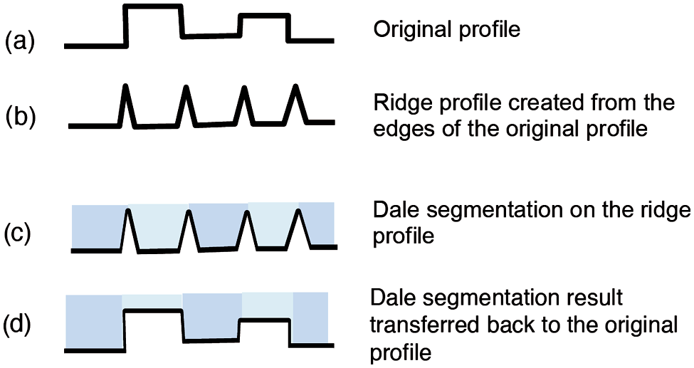
Steps of range image segmentation based on edge preprocessing and morphological dale segmentation.
The final result of segmentation, as required, is a partitioning of the original range image where each region (partition/segment) is characterized by roughly uniform height properties. As stated earlier, this is a low-level partitioning, since the regions have not been associated to known features yet.
Feature identification
Each region obtained by segmentation must be identified as an instance of one of the features belonging to the nominal model. This is done by aligning the segmented image (also referred to as the segment map) to a labeled feature map, as shown in Figure 5 and illustrated in the following text.
Registration of the segment map and the labeled feature map for the identification of measurand features: (a) segment map; (b) segment edge map; (c) labeled feature map; (d) labeled feature edge map; (e) registration through edge alignment and assignment of labels to segments by pixel voting.
The labeled feature map (Figure 5(c)) is a 2D geometric model that collects the 2D nominal shapes of the relevant areal features (i.e. the projections of any surface feature onto the xy plane) existing on the measurand surface, each associated to a unique identifier (label). The labeled feature map is assumed available as a companion of the CAD model of the part or device, the shape of each areal feature being defined by a closed loop of straight and curved line segments.
Alignment is achieved by solving a 2D registration problem based on finding the rotation and translation transform that minimizes the cumulative distance (in the least-squares sense) of two edge maps: one is a raster image obtained by extracting the boundaries of the segments from the segmentation map (the segment edge map, Figure 5(b)), the other is the collection of 2D straight and curved segments extracted from the labeled feature map (referred to as the labeled feature edge map, Figure 5(d)).
Once the registration is complete, each segmented region is assigned a label (Figure 5(e)) based on an original voting process, where each pixel belonging to the segment map votes for the label of the region it falls into within the labeled feature map after registration. The voting process is better illustrated with the help of Figure 6.
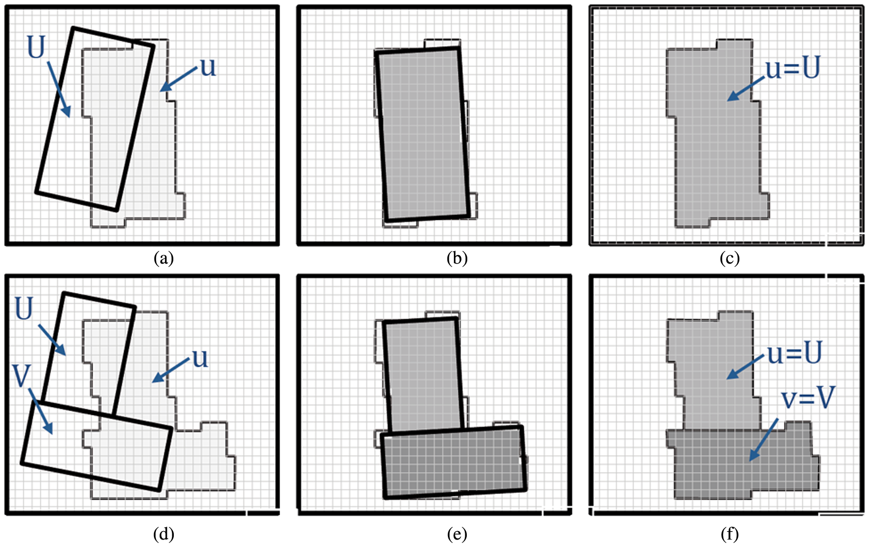
Voting process: (a), (b), (c) segment u is associated to feature U owing to strong voting consensus (most u pixels fall within the U boundaries); (d), (e), (f) owing to voting disagreement (u pixels fall within U and V boundaries), segment u is split into two sub-regions u and v, and they are independently associated to features U and V.
In Figure 6(a), (b) and (c) the simplest scenario involving a voting process is illustrated: in Figure 6(a) a segment (u) obtained by segmentation of the range image is shown, together with the polygon defining the edge of feature, U, in the misaligned labeled feature edge map. In Figure 6(b), after registration, each pixel of the segment “votes” for U if it falls within the polygon, otherwise it votes for the background. In this case only a few pixels vote the background, their number being below a predefined threshold. Therefore, in Figure 6(c) since there is a strong consensus of votes in favour of U, the voting process terminates and the segment u is associated to the feature U.
In Figure 6(d), (e) and (f), a slightly more complex situation is shown where, after alignment, segment u falls in the domain of the two features U and V. In Figure 6(e), aside from a few usual votes falling into the background, two significant groups of voters are formed, both above the rejectability threshold, thus creating a disagreement. In this case, the segment u is automatically partitioned into u and v, by using the voting results to identify the split line; then each sub-region is again individually subjected to voting. In the example, the two sub-regions end up being associated to the features U and V.
With an appropriately preset threshold, the voting process is fairly robust to both alignment error and variations between nominal and acquired geometry.
At the end of feature identification the following goals are achieved.
The acquired, rectangular region is localized within the nominal geometry: this is useful because the acquisition region may not entirely correspond to the measurand region, which should be verified (see previous comments on lateral resolution and range, and see Figure 1), and because some misalignment could exist owing to imprecise positioning of the physical specimen in the instrument measurement volume.
A mapping is established between each non-ideal surface feature (associated to a partition in the segment map) and the corresponding ideal surface feature (associated to a labeled region in the label map), which will be useful for the association step later on.
It is possible to determine what parts of the verification process will be actually achievable, since features and characteristics falling partially or entirely out of the acquired region will be discarded from the analysis.
Segment postprocessing for error compensation
Before the data points contained within each segment can be used to populate non-ideal surface features, post-processing must be applied in order to avoid introducing additional sources of error. At this stage, the dataset preprocessed by interpolation has served its purpose (segmentation), and is replaced with the one preprocessed by voiding the artefacts (whenever possible, as illustrated earlier). Notice that the segmentation and feature identification results apply to both datasets indifferently. Postprocessing involves compensating for distortions caused by levelling by projection. It basically consists in the following steps (Figure 7).
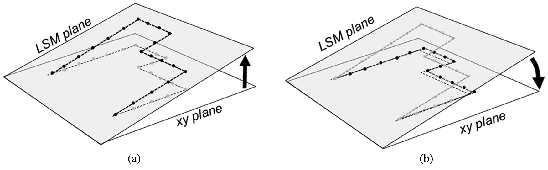
Procedure for compensating the distortions introduced through levelling by projection. For the sake of simplicity, a point subset is shown that follows a recognizable feature boundary aligned to the LSM plane: (a) inverse z-projection to bring the LSM plane back into its original position; (b) rotation to align the LSM plane to the xy plane.
Turn each range image subset (segment) into an unstructured set of x,y,z points.
Apply the inverse z-projection transform to the points so that they return to their original unlevelled positions (Figure 7(a)).
Apply the forward rotation and translation transform to re-level the points (Figure 7(b)).
Since rotation breaks the uniform grid layout of the image pixels, post-processing output is always encoded as a set of sparse points. Since the final result is not an image any more, no image processing technique can be applied beyond this point, and only algorithmic solutions for processing generic point clouds can be adopted.
Populating the non-ideal surface features
Once the points belonging to each segment have been identified as associated to an ideal surface feature, and once they have been compensated for levelling distortions, they can be extracted as a separate subset and used to populate the corresponding non-ideal surface features (Figure 2(f)). Given that segments are mapped to areal features, only non-ideal surface features can be created this way.
Creation of non-ideal derived geometric features
Additional non-ideal geometric features (e.g. points, lines) can be derived from the available surface features. For step-like structured surfaces, the most common examples for this type of feature are geometric elements related to the xy boundary profile of the protruding or recessed volumetric features. These elements are important because they provide the necessary information through which most linear dimensions on the xy plane can be analysed. The extraction of an xy boundary profile (set of non-ideal line features) from a non-ideal surface feature defined by a set of points consists of identifying the boundary points of the set projected onto the xy plane. Thus, it is about solving a well-known problem of 2D computational geometry (i.e. finding the boundary points of an unstructured 2D point set). In the proposed approach, the outer boundary of any point set is found by inspecting the topology of the Delaunay triangulation of the projected points. Inner boundaries (existing in case the non-ideal surface completely encloses additional surfaces in the xy plane) are more challenging, and are not found directly, but as the outer boundaries of the enclosed non-ideal surfaces.
Finally, it should be noted that, like the non-ideal surface features, the xy boundary profiles are populated only by points; that is, non-ideal geometric features are not subjected to reconstruction (ISO 17450-1) to obtain continuous geometry at this stage.
Step 4: association and final verification
In the final step of the proposed approach, non-ideal geometric features (defined by points, as illustrated in the previous section) are fitted to their ideal counterparts (defined by continuous analytic geometry) (Figure 2(g)). The correct pairing between each ideal and non-ideal surface feature is assumed known as a byproduct of areal feature identification (see previous step). The remaining task is to fit each ideal geometric feature to the subset of points corresponding to the paired non-ideal feature. Since the ideal geometry is constrained in size (because it belongs to the nominal model), this is essentially about solving another rigid registration problem, which, in ISO 17450-1 terminology, is the equivalent to identifying an additional situation characteristic to localize the non-ideal feature with respect to the ideal one. Registration at this stage is implemented by appropriate fitting models, which depend on the type of feature involved (point, line, surface), and on the type of specification associated with the ideal feature (dimension or zone). Thus fitting may typically follow a least-squares criterion, or a non-least-squares one such as Chebyshev, or mating envelope (maximum inscribed or minimum circumscribed) depending on the specific requirements of the specification.
Regardless of the adopted fitting criterion, once the association step is complete, it is possible to achieve the final goal of the verification process by quantitatively assessing the deviations (ISO 17450-1), and thus verify whether each geometric feature conforms to the assigned specifications.
Application of the proposed verification approach to a test case
To validate the proposed approach, its application to an example class of micro-fabricated, high-precision parts characterized by step-like features is illustrated in the following sections. The whole data processing procedure was implemented in prototype form in MATLAB. 16
Test case
Thin-foil targets are micro-fabricated parts used in laser-driven ion acceleration experiments: when a high-intensity laser pulse is focused on the front surface of a target, electrostatic fields and heated plasma are created resulting in ion acceleration from the rear surface of the target. 17 An example silicon nitride laser target, manufactured by the Micro and Nanotechnology Centre at STFC (Science and Technology Facilities Council), UK, is shown in Figure 8(a). The target is the central disk (32 μm nominal diameter, 100 nm nominal thickness) suspended by spokes at the centre of a circular through hole (305 μm nominal diameter) created onto a base structure. Similar to many micro-electromechanical systems (MEMS), the micro-part is produced by a sequence of chemical vapor deposition (CVD), photolithography and etching operations. Currently the verification process is mainly qualitative, and based on visual inspection of SEM images. The micro-part can be seen as a structured surface with step-like features; a solid CAD model of the part is visible in Figure 8(b) (ISO 17450-1 ideal model).
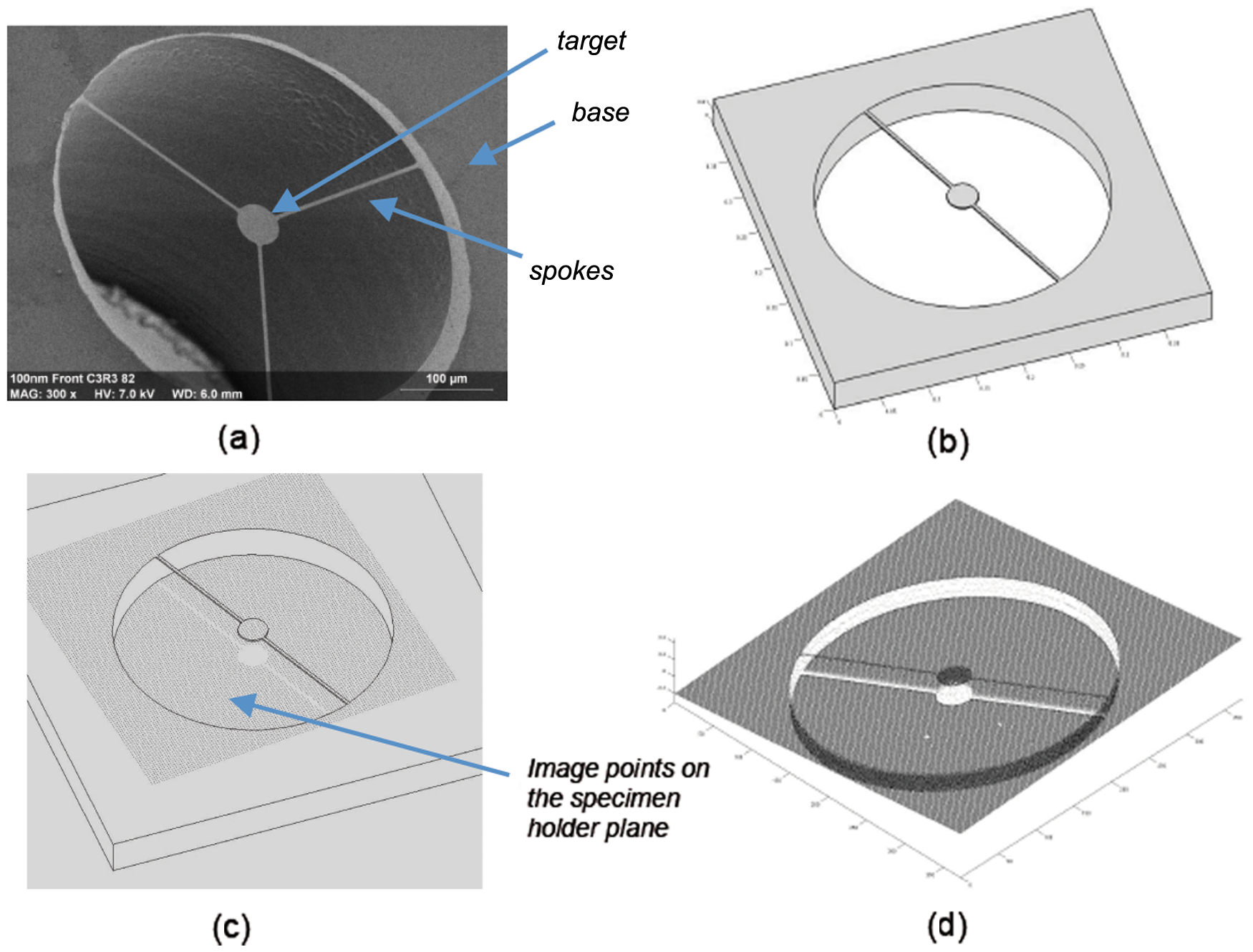
Thin-foil target: (a) SEM image of a three-spokes variant (however, the two-spokes variant was analysed in this work, as shown in the following subfigures); (b) CAD model of the two-spokes variant (ideal surface model); (c) simulation of surface acquisition through imaging: the part is shown placed on the specimen holder plane and part of the acquired points fall onto it; (d) the real, raw dataset acquired with a WLSI 3D profilometer: 1024 × 1024 points on a regular grid with 363 nm × 364 nm x,y spacing, resulting in a definition area of 372.29 μm × 372.64 μm.
Planning and execution of the measurement process
The top surfaces of several microtarget specimens were acquired with a commercial WLSI optical 3D profilometer (Taylor-Hobson CCI 3000 8 ). Since the specimens were positioned with their top surface approximately parallel to the xy plane of the measurement instrument, owing to the limitations of unidirectional observation no data could be acquired from the vertical walls and from the bottom surfaces of the target and spokes (see Figure 8(c)). An example point set resulting from the measurement of a two-spokes variant of the microtarget is shown in Figure 8(d). Since the target is suspended onto a through hole, the dale regions visible in Figure 7(d) actually belong to the specimen holder plane (see again Figure 8(c)).
The profilometer features a 1024 × 1024 CCD camera and for this test was equipped with a 50× Mirau objective, yielding a lateral range of 372 μm × 372 μm, sufficient for acquiring the entire topography of the target, and a lateral sampling resolution of approximately a 0.363 μm × 0.364 μm (pixels are slightly rectangular). With a numerical aperture (NA) of 0.55, the optical lateral resolution provided by the objective lens according to the Rayleigh criterion is about 0.5 μm, which becomes the leading criterion in determining the minimum resolvable distance. In working terms, for dimensional metrology this means that three pixels in the CCD output are needed to safely assess two adjacent heights as independent measurements.
The vertical resolution provided by the 50× objective is < 0.1 nm, which is adequate for evaluating the topography of the specimen top surfaces, and a vertical range compatible with the depth of the through hole.
Maximum detectable slope for the objective is approximately 27°, which means that no reliable information can be collected for the specimen side walls. Of course no information could be acquired from the bottom surfaces of the target and spokes, being completely inaccessible from the direction of observation.
Ideal and non-ideal models and features
In order to apply the proposed verification approach, an ideal surface model can be built starting from the available information concerning the main shape and nominal dimensions of the microtarget. As often happens for this class of devices, 13 no tolerancing information is defined, and therefore none has been considered. The ideal model is conceptually partitioned into the ideal volumetric features: target, spokes and outer rim (see again Figure 8(a) and (b)), each being bounded by horizontal surface features at the top and bottom, and by vertical surface features (either planar or cylindrical) at the sides. A skin model can be imagined available, which reproduces the same structure and organization of the ideal model. However, no knowledge about expected variations is incorporated into the skin model at the moment, except for measurement data as shown later. It should be noted that the proposed approach may also be used to collect information about part variation, and thus support the development of models describing expected variation, to be incorporated in the skin model.
As indicated in Figure 2, albeit the non-ideal model includes the complete set of surface features (Figure 2(d)), some of them (i.e. vertical side walls and shadowed surfaces) will not be populated by measured points (Figure 2(f)). For the test case, the verification process is designed to take this into account, and targets only the top specimen surfaces and the related xy boundary profiles. The following feature characteristics (intrinsic and situation) are investigated.
xy Boundary profile of the target (ideal feature: circle): diameter.
xy Boundary profile of the through hole outer rim (ideal feature: circle): diameter.
Distance between target and outer rim circle centres.
xy Boundary profile of each spoke (ideal features: two parallel straight lines): width, angular orientation with respect of the x axis.
Flatness of target, spokes and base top surfaces.
Preprocessing
Missing data is removed by interpolation with a median operator computed on a 3 × 3 moving window. Batwings (Figure 9(a)) are identified with a 7 × 7 median filter, and a threshold for outlier detection set at 2*SD (see the preprocessing step for details). In Figure 9(b) the result of artifact replacement with the median surface is shown: notice that the batwing effect is not completely removed, thus height measurements taken in close proximity of a step boundaries are not to be considered reliable.
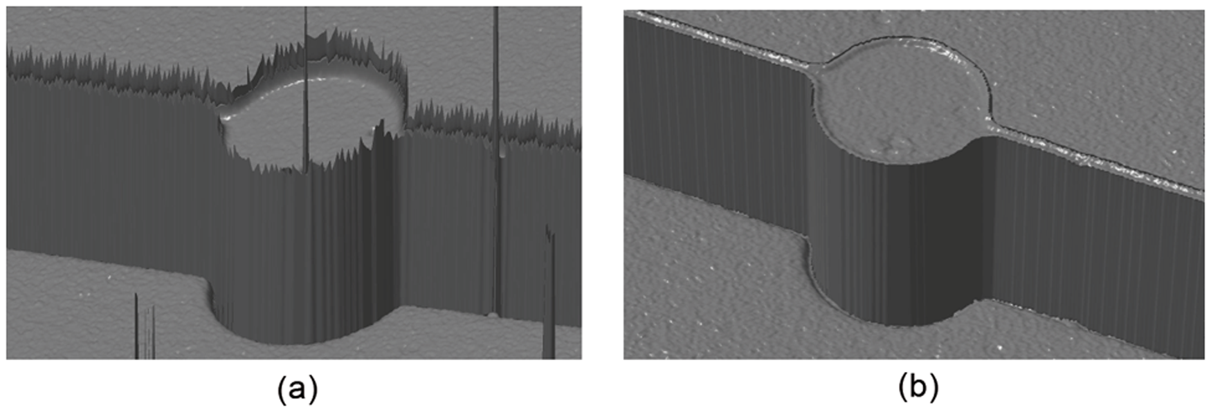
Measurement artifacts identification and removal: (a) batwings at the top and bottom of step-like transitions; (b) batwings replaced by the interpolation of the neighbours with median operator.
Extraction
The result of edge-preprocessing plus morphological dale segmentation is shown in Figure 10(a). Notice that target, base and spokes have been recognized as a single segment since their top surfaces have approximately the same height and are not mutually delimited by steps. The two visible portions of the specimen holder plane are also visible in the segmentation result as two topologically disconnected dale-like regions. The labelled areal feature map is shown in Figure 10(b). In the map, which is assumed available as part of the nominal geometry, the specimen-holder regions have been classified as “not relevant” for the verification process, while the target, spokes and base are defined as separate features, as they are supposed to be. The registration of the segmentation map to the labelled feature map is done by aligning the relevant edges according to a two-step process: coarse alignment through principal component analysis (PCA), 18 and fine alignment through the iterative closest point (ICP) algorithm. 19 In Figure 10(c) the application of the voting algorithm onto the aligned geometries leads to the final feature identification result. It should be noted in particular that the target, spokes and base surface features are now correctly identified as separate features.
Steps of the extraction process: (a) segmentation map; (b) labelled feature map; (c) areal feature identification by registration of the two maps.
In the tests made on the microtarget datasets, segment post-processing for levelling error compensation (projection versus rotation) always revealed a negligible difference in the final point coordinates (maximum lateral shift detected < 0.1 nm, which is three orders of magnitude smaller than lateral resolution). Also, the comparison of the results obtained by levelling with a global LSM plane (i.e. defined by considering all the available data points) and with a local LSM plane (computed with the points of the outer-rim region only, as obtained by segmentation) yielded negligible differences.
After post-processing, the point sets are used to populate the corresponding non-ideal surface features. Then, the non-ideal, derived surface features, i.e. the xy feature boundary profiles of the target, spokes and base outer-rim are populated by the outer boundary points of each segment.
The entire extraction process can be summarized by focusing on a topographic detail, as shown in Figure 11. In Figure 11(a) the original “cleaned” range image is shown: portions of the outer rim and of a spoke are visible. In Figure 11(b) a colour map representing the results of the voting process (feature identification) is shown overlaid onto the original surface. Outer rim and spoke regions are correctly discriminated. In Figure 11(b) an additional small region is shown, created at the junction between spoke and outer rim by dilating the pixels located on the partition line through a morphological dilation operator. 14 This region is referred to as a region of transition between features and its role is illustrated in the following. In Figure 11(c) the region surrounding the outer rim is highlighted, these are the points used to populate the corresponding non-ideal surface feature. In Figure 11(d), the boundary of the region is extracted, corresponding to the approximate location of the outer rim edge (derived feature). At this stage, the region of transition previously shown in Figure 11(b) is used to delete potentially less reliable boundary points located at the transition with the spoke. After post-processing (not shown), the remaining boundary points are used to identify the least-squares best-fit circle for the outer rim edge, shown in Figure 11(e); the best-fit circle is rendered slightly raised above the surface for better clarity. The step shown in Figure 11(e) actually corresponds to the ISO 17450-1 association operation (see also Figure 2), and will be detailed in the following section.
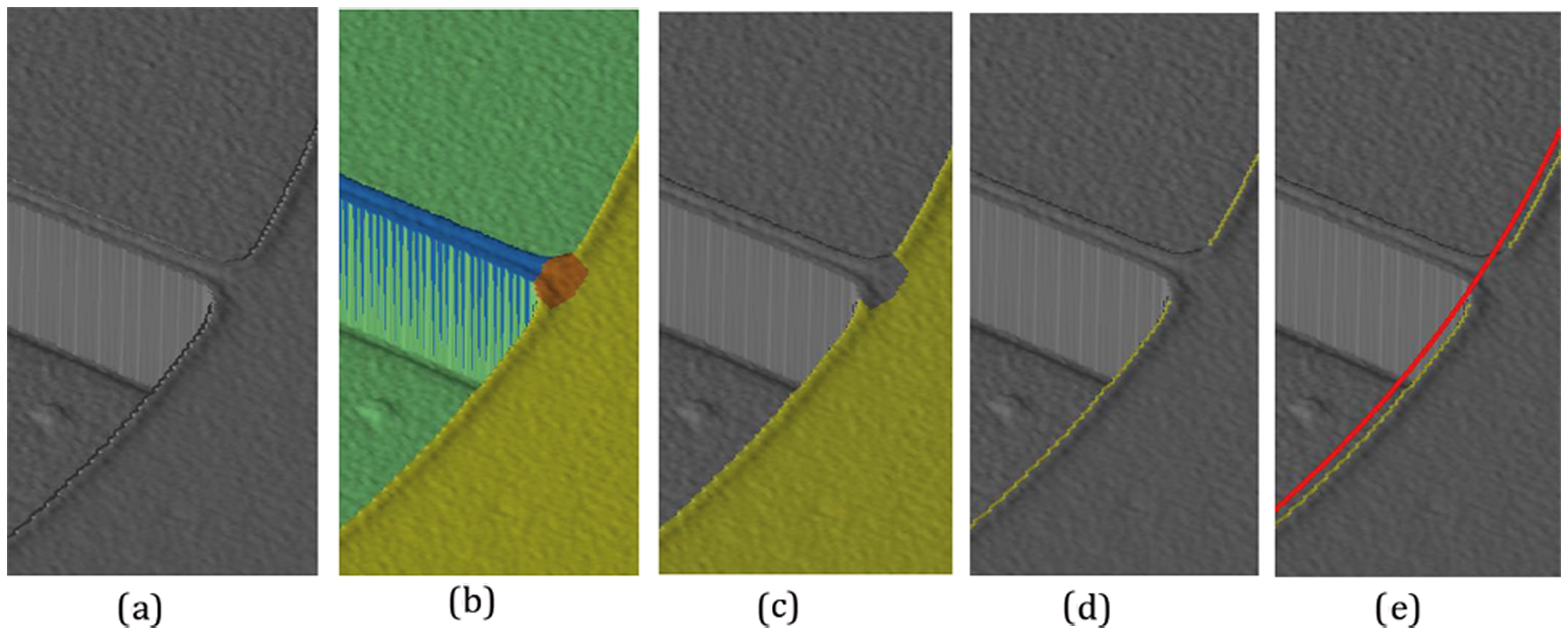
Steps of the extraction process, observed on a local topographic detail: (a) original surface; (b) discrimination of features; (c) selection of the region surrounding the outer rim edge; (c) identification of boundary points; (d) best-fit circle for the outer rim edge.
Association and final verification
As preliminarily illustrated by the example in Figure 11(e), at association each non-ideal feature is fitted to its ideal counterpart. In Figure 12(a) the complete result for the test case is presented, where the ideal xy boundary profile elements (circles and straight lines) are shown, each fitted to the subset of boundary points contained within the corresponding non-ideal geometric feature. Since no geometric tolerance is currently involved in the specifications, 2D least-squares fitting onto the xy plane is adopted by default for association. Once the ideal geometries are properly fitted, it is possible to analyse the deviations of the non-ideal xy boundary profiles of the target, spokes and base outer-rim.
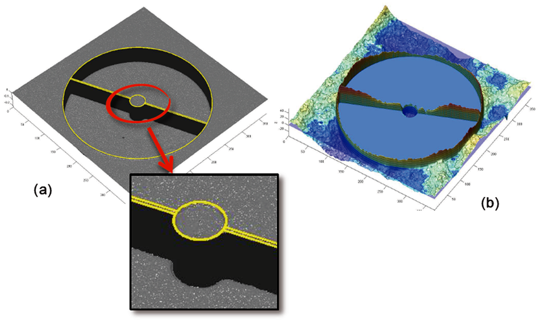
Association results and assessment of deviations: (a) ideal geometric features (xy boundary profile elements) fitted to their non-ideal counterparts (unstructured point sets extracted from non-ideal surface feature boundaries); (b) magnified deviations of the measured base surface with respect to the ideal plane surface feature (shown in transparent colour).
Quantitative results obtained by the measurement process are shown in Table 1. These are essentially geometric properties computed from the best-fit geometries, compared with nominal data known for the target device. The concentricity error is measured as the Euclidean distance between target and outer rim centres. The angle between spokes is measured between spoke medial axes, each medial axis being the symmetry line between the two best-fit edges of the spoke. The width of each spoke is computed as the mean distance between spoke edges (not necessarily parallel), measured orthogonally to the medial axis.
Measured and nominal values associated to the xy boundary profile elements.
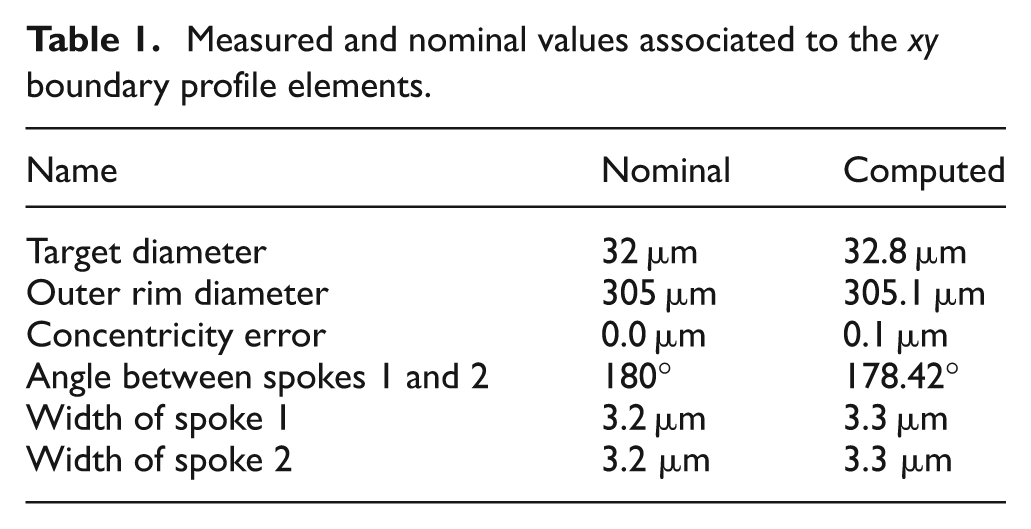
To analyse the flatness of the base, spokes and target top surfaces (even though a flatness tolerance is not defined in the nominal model), the related non-ideal surface features are fitted together to the same ideal global plane. The resulting deviations can be visualized with an enhanced vertical magnification and colouring proportional to deviation, as shown in Figure 12(b). Notice that the target top surfaces is slightly recessed with respect to the ideal plane, probably owing to its thin-foil, suspended structure slightly collapsing under its own weight; the base surface is also slightly bent downwards. Residual batwing effects are still visible at such high magnification, and make less reliable in particular the assessment of the topography of the top surfaces of the spokes.
Conclusions
A novel approach has been proposed for the characterization of critical dimensions and geometric errors, suitable for application to micro-fabricated parts and devices characterized as step-like structured surfaces. The approach is based on the framework proposed by the ISO 17450-1 standard for geometric verification, while at the same time addressing the most relevant and peculiar aspects related to dimensional metrology of step-like structured surfaces, and considering in particular the main issues arising when using optical 3D profilometers to acquire the geometric information.
The proposed procedure is of general applicability. To demonstrate it, an application to the measurement of thin-foil laser targets for ion acceleration experiments has been illustrated. While the solution is demonstrated applicable to this class of dimensional metrology problems, critical issues related in particular to the assessment of measurement uncertainty remain to be addressed and are the subject of future investigation.
Footnotes
Funding
The authors gratefully acknowledge the UK’s Engineering and Physical Sciences Research Council (EPSRC) funding of the EPSRC Centre for Innovative Manufacturing in Advanced Metrology [No. EP/I033424/1].