
Abstract
Tool wear prediction is paramount for guaranteeing the quality of the workpiece and improving lifetime of the cutter. However, the multicollinearity between the extracted features deteriorates the prediction accuracy. To overcome this, a partial least square regression-based method is proposed. The main characteristic of partial least square regression is that the regression analysis is realized in the principle component space so that multicollinearity between the input variables can be avoided. To testify the correctness of the proposed method, the milling experiment is preceded and the dynamic cutting force is collected to depict the variation of the tool wear. Moreover, Monte Carlo cross validation is adopted to improve the robustness of partial least square regression. The analysis and comparison between the partial least square regression model and the multiple linear regression model shows that the presented method can get more accurate results.
Keywords
Introduction
With the development of modern manufacturing industries, more attention is focused on how to minimize cost and maximize productivity. Tool wear is one of major obstacles to realize large scale automation and minimize human intervention. 1 In comparison with tool status classification, tool wear prediction is preferred in some cases because the accurate tool wear value can be estimated so that the further process optimizing and control strategy can be taken in time. Previouly, many researchers have focused much energy on effective and accurate prediction of the tool wear value and multiple linear regression (MLR) is one of the commonly used methods to predict the tool wear value based on sensory signal. Jacob et al. 2 built a MLR model to predict the tool wear based on the average force and the average peak force. Bhattacharyya et al. 3 proposed a two-stage model in which the MLR model was used in the first stage to relate the selected features to the tool wear value so that the tool wear value was predicted accurately. Li et al. 4 realized the tool wear prediction with the combination of the MLR model and the wavelet-based features. These successful applications demonstrate the effectiveness of the MLR method. However, because all feature variables depend on the variation of tool wear status, the colinearity exists inevitably among them. Moreover, the feature vectors under the same tool wear value usually fluctuate within a certain scope because of the disturbance of the noisy signal and the complexity of tool wear topology. In this situation, the model coefficients of the MLR may change erratically in response to small changes in the model or the data, which will deteriorate the prediction accuracy correspondingly.
In this article, to overcome the shortcomings of MLR and improve the accuracy of tool wear prediction, a partial least square regression (PLSR) model is presented. PLSR combines the characteristics of principal component analysis and the MLR model. The main advantage is that the regression analysis is established in the principal component space in which the variables are independent from each other. Therefore, the colinearity between the selected variables can be avoided, which will improve the prediction accuracy greatly. The PLSR method has been adopted in many aspects, such as predicting infrared spectra, 5 ripening time of Manchego cheese, 6 couples mental health 7 and time series modeling of process data. 8 However, to the author’s knowledge, the evaluation of using PLSR to overcome the multicollinearity in the field of continuous tool wear prediction has not been reported. To testify the effectiveness of the proposed method, milling experiments of Titanium alloy are carried out and sixteen harmonics features are utilized to predict the tool wear value using the PLSR model. Moreover, the Monte Carlo cross validation (MCCV) method is also adopted to improve the robustness of the prediction model. The analysis and comparison between PLSR and MLR shows that the combination of PLSR with MCCV is more accurate to realize online tool wear prediction.
This article is organized as follows. The principle of PLSR and MCCV is given first. The experiments and harmonics based feature extraction method are then described. The analysis of the variation of extracted features shows that the multicollinearity exists between different harmonics. Based on MCCV, PLSR is utilized to build the relationship between the tool wear value and the harmonic features. To make a comparison, the MLR is also adopted to predict the tool wear value using the same data as the training and test samples. The analysis and comparison of different performance criteria show that the PLSR outperforms the MLR method. Some useful conclusions are given in the last section.
Principle of PLSR modeling and MCCV
Principle of PLSR modeling
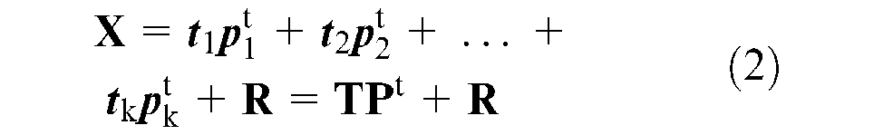
To avoid the deterioration of the tool wear prediction accuracy because of the multicollinearity between the selected feature variables, the PLSR model is adopted that is built according to the following calibration model 9

where E(.) and Cov(.) denote the expectation and covariance, respectively. To extract the partial least square (PLS) components, the observation matrix
where

where α is the simplification of

The number of components k is also called the dimension of the model. The least square solution of equation (4) is calculated by

and the fitted value of

where

Therefore, the PLS estimator

The detailed algorithm of PLSR modeling is described in Qingsong and Yizeng. 9
Principle of MCCV
Although PLSR is an effective method to get rid of multicollinearity in the explanatory variables and realize the accurate modeling, it is difficult to determine the suitable number of latent variables so as to obtain the best predictive ability. Here, MCCV is presented to perform the cross validation several times iteratively based on the Monte Carlo algorithm. At each time, it splits the training samples into two parts S c and S v randomly and this process is repeated L times in which the MCCV criterion is defined as 9
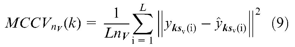
where
Experimental set-up and feature extraction
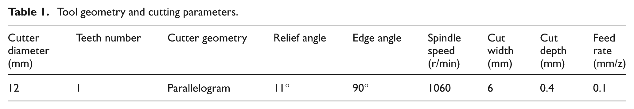
As shown in Figure 1, a milling experiment of Ti–6Al–4V titanium alloy was conducted in a Makino vertical machining center and the cutting forces generated during the machining process are measured by a three-axis piezoelectric dynamometer and collected by a data acquisition card (sampling at 10 kHz). The tool geometry and cutting parameters are described in Table 1. The tool wear status is measured by an optical microscope after every cutting pass. As shown in Figure 2, the cutter wear appeared around the tool nose zone. Therefore, the maximal vertical length of this area was measured to depict the tool wear status. Finally, 38 cutting passes were achieved and the force during each pass was collected continuously during the machining process. Because the fore signals are polluted by the noisy signal, it should be preprocessed first by getting rid of the trend item and the wild data. The filtered waveform of the cutting force in the feed direction and its amplitude spectrum are illustrated in Figure 3, from which we can see that the signal displays periodic characteristic and the dominant frequency components in the spectrum representation of cutting force are around the tooth passing frequency (TPF) and its integral multiple harmonics. Therefore, the amplitude corresponds to the TPF and its harmonics are selected as the feature vectors to depict the variation of the tool wear. The TPF can be calculated by
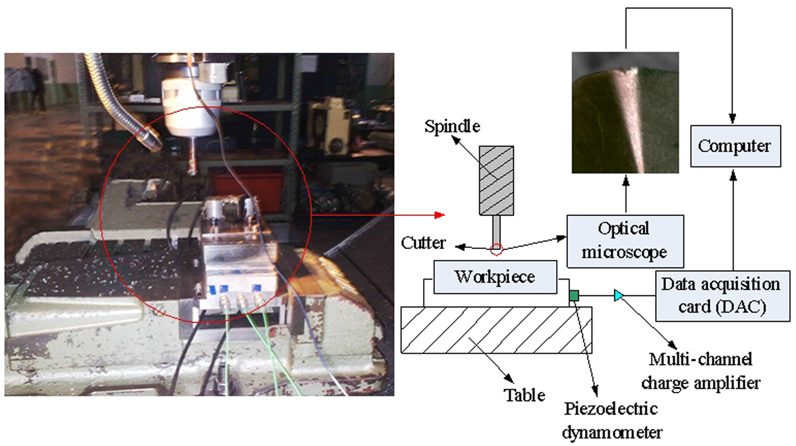
Schematic diagram of the experimental set-up.
Tool geometry and cutting parameters.
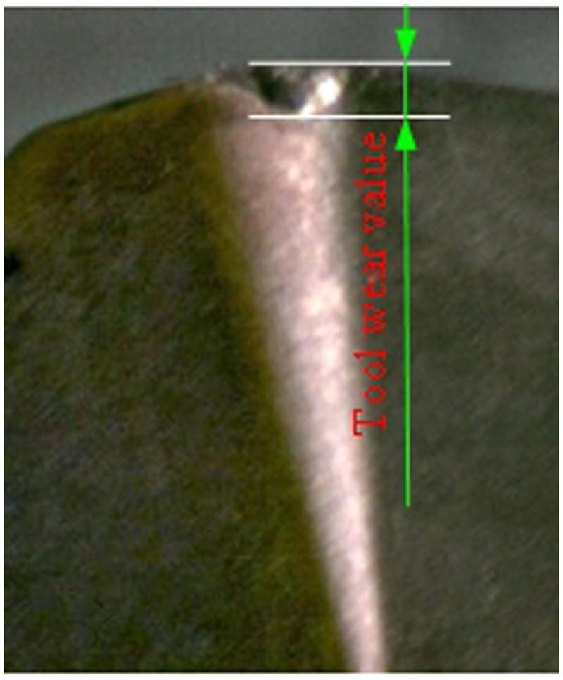
Sketch of tool nose wear measurement.
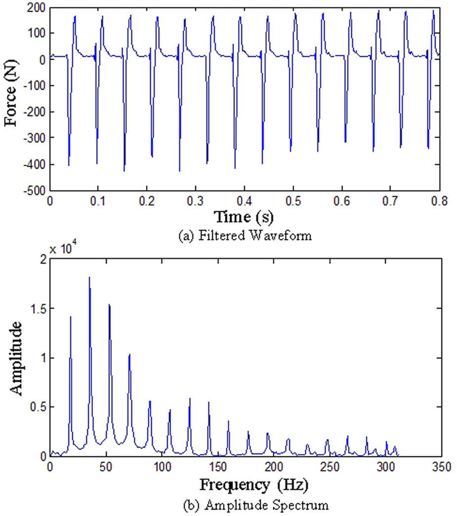
Waveform and spectrum of milling force signal.

It has been proven that the amplitude of the cutting harmonics increase with the processing of the tool wear status.10,11 Because the TPF and its harmonics are within the lower frequency band, the force signal is first decomposed into different scales with discrete wavelet decomposition in which the coefficients in the jth levels can be written as 12
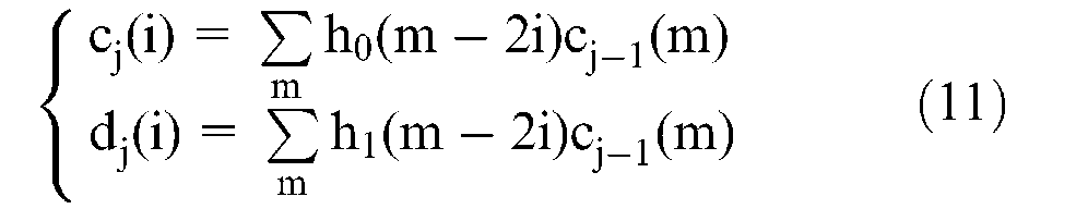
h0 and h1 are the low-pass and high-pass filters related to the wavelet function, and m and i are the index of the elements in the signal. Then, the amplitude spectrum of the low frequency signal c(i) at certain scale j is calculated by fast Fourier transform (FFT) analysis and the peak amplitude value around the TPF and its integral multiple harmonics can be obtained and organized as feature vectors. The whole flowchart of the feature extraction is demonstrated in Figure 4.
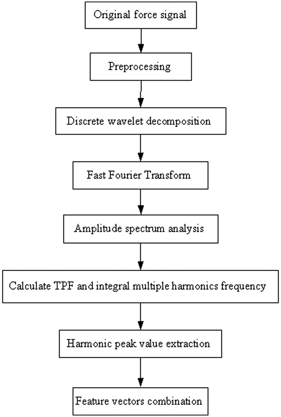
Flowchart of harmonic-based feature extraction.
In this article, the scale of wavelet decomposition is selected as three, therefore the frequency band scope of the low frequency signal is within 0∼1.25 kHz. Because the amplitude of the harmonics in the spectrum graph decrease with the increase of the harmonic order on the whole and the amplitude corresponding to the first 16 harmonics are larger than the others, obviously, these amplitude values are selected and organized as the feature vector to depict the variation of the tool wear status. To show the generalization of the proposed model, the cutting force signal is first divided into 40 segments with the length of 8000 data points. So the total number of samples for each tool wear status is 40. The variation of the several selected features with the tool wear value is illustrated in Figure 5 by means of box plot, in which (a), (b) and (c) denotes the 1st-order harmonic feature, the 6th-order harmonic feature and the 11th-order harmonic feature, respectively. For each box, the central mark is the median value and the edges of the box are the 25th and 75th percentiles. The whiskers extend to the most extreme data points, which are not considered as outliers and the outliers are plotted individually, which are labeled as ‘+’. It can be seen that the median value of the harmonic features increase with the increasing of the tool wear value monotonically and these features share the common trend. To further analyze their relationship, the correlation coefficients of different harmonic features are calculated and some of the results are listed in Table 2.
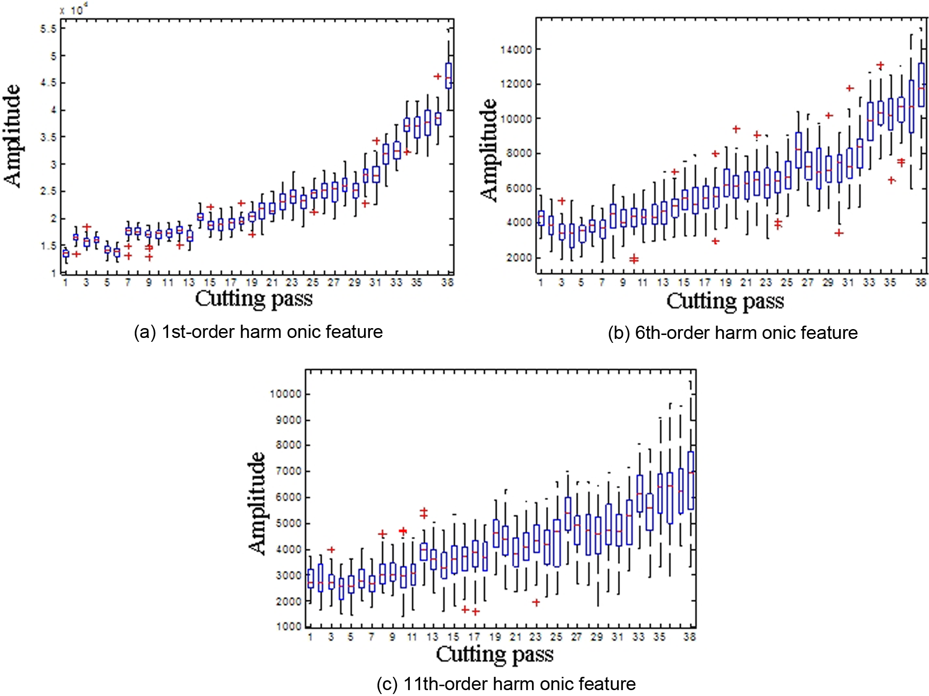
Feature variation under different orders.
Some of the correlation coefficients between different harmonic features.
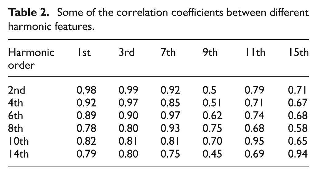
It can be seen that these feature vectors are highly correlated. When they are utilized as the predictor variables, multicollinearity is introduced between them unavoidably, which will deteriorate the prediction accuracy correspondingly. Therefore, to improve the prediction accuracy and robustness, the PLSR is adopted in the following section to predict the tool wear value and make comparison with MLR.
Tool wear prediction using PLSR and comparison with MLR
MCCV
In this section, PLSR is used to build the regression model and realize the prediction of tool wear based on MCCV. Here the repetition times of the MCCV are set to 500 and the maximum number of the latent variables is 16. The variation of the MCCV criterion with the increase of latent variables is illustrated in Figure 6. It can be seen that the value of the MCCV criterion goes down quickly as the number of component increases. However, after the number of the latent variables is larger than 10, it increases slightly. Therefore, the optimum number of the explanatory variables for PLSR is selected as 10.
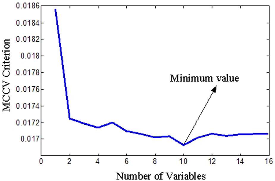
Variation of MCCV criterion with the number of latent variables.
Comparison of PLSR with MLR
After the optimum number of the latent variables is determined, the PLSR can be realized for online prediction of the tool wear value. Moreover, MLR is also adopted based on the same data here to make a comparison with the PLSR. To compare the performance of these two methods intuitively, four indicators are presented to depict the global prediction capability of the proposed method. The first is the average absolute error in predicting the tool wear value 13
where
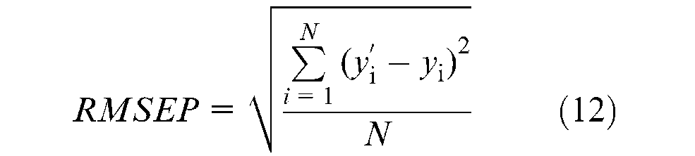
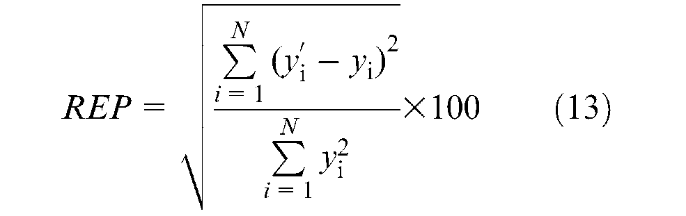
The second is the relative error of prediction of the dependent variable in percentage (REP), which is calculated as 13
The third is the accuracy factor (A f ), which indicates the spread of the results about the prediction 13

The above indicators illustrate the accuracy of the model in different aspects. The smaller the indicator is, the higher the accuracy. The fourth is called the coefficient of determination (R2), which represents the percentage of variability that can be explained by the model 13
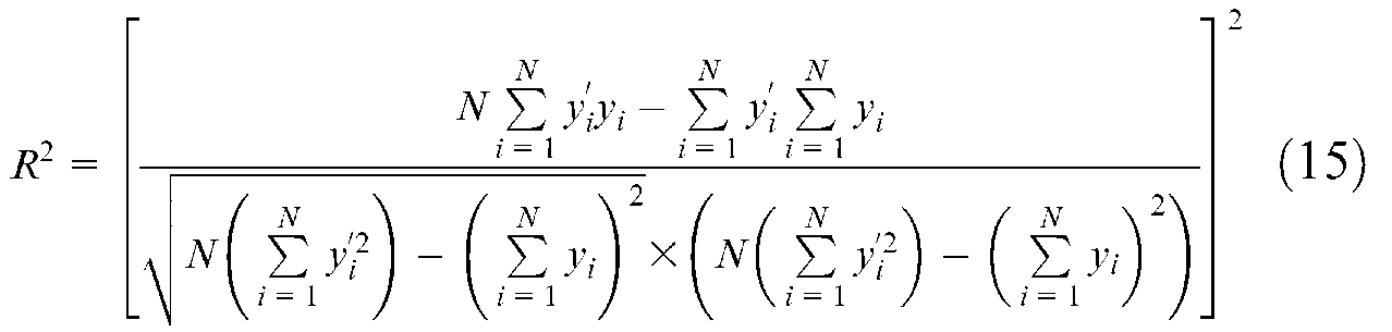
The larger value means that the model has a stronger ability to reflect the relationship between the features and the tool wear status.
Based on these performance indicators, the numerical comparison of the PLSR and MLR under the same number of explanatory variables is realized and the results are listed in Table 3. It can be seen that the prediction accuracy of the PLSR is higher than MLR. To demonstration the difference of the prediction results between the PLSR and MLR more clearly, the comparison of the measured and predicted tool wear value under different cutting passes is illustrated in Figure 7. It can be seen that the accuracy of PLSR method is higher than MLR at both the beginning and final stage of the tool wear process. Therefore, it can be concluded that the PLSR has a strong ability to overcome the influence of multicollinearity so as to realize a more accurate online tool wear prediction.
Performance comparison of PLSR with MLR.
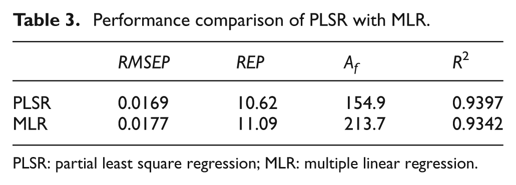
PLSR: partial least square regression; MLR: multiple linear regression.
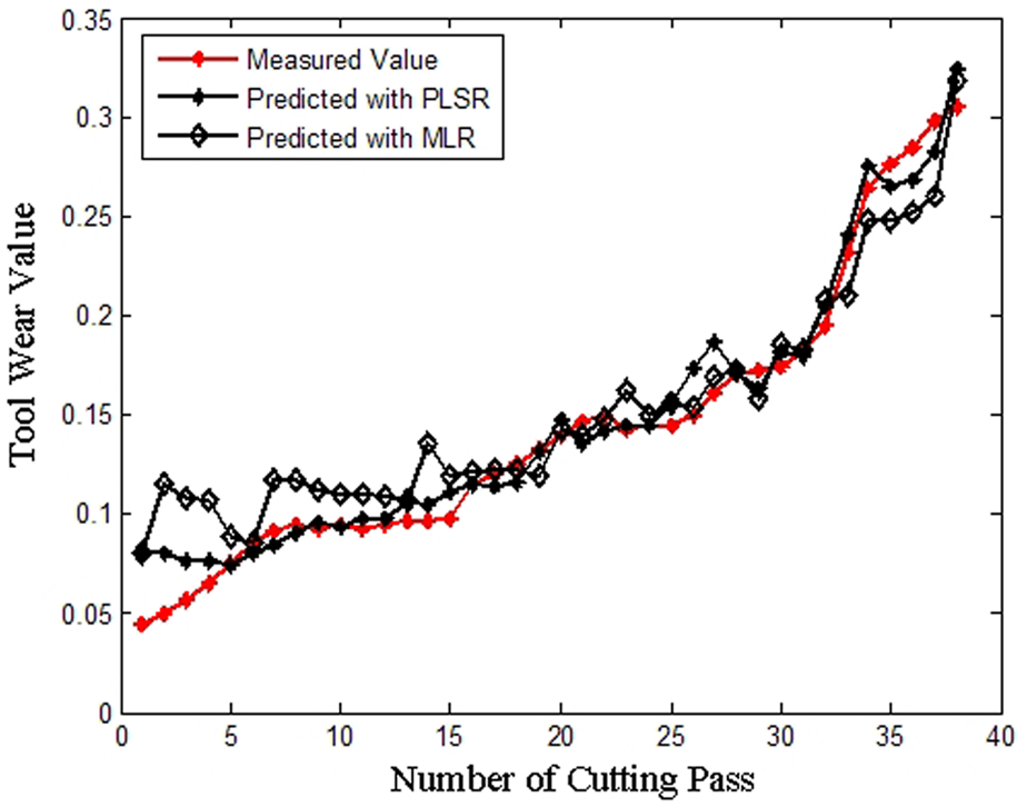
Comparison of predicted tool wear with measured value.
Conclusions
In this article, to overcome the influence of multicollinearity and improve the accuracy, a PLSR model is presented to realize continuous tool wear prediction. The main characteristic of the PLSR is that the model can be built in the principal component space so as to avoid the multicollinearity among the input features. To testify the effectiveness, a milling test is carried out and the harmonic features extracted from the milling force signal are adopted to depict the variation of tool wear status. By comparing several performance indicators and analyzing the prediction curve, it can be concluded that the PLSR model outperforms the MLR for the accurate prediction of tool wear status. This method casts new light on the online accurate prediction of tool wear in the industrial environment.
Footnotes
Funding
This project is supported by National Natural Science Foundation of China [51175371].