Sage Journals: Discover world-class research

Abstract

This paper reports an experimental method to estimate the convective heat transfer of cutting fluids in a laminar flow regime applied on a thin steel plate. The heat source provided by the metal cutting was simulated by electrical heating of the plate. Three different cooling conditions were evaluated: a dry cooling system, a flooded cooling system and a minimum quantity of lubrication cooling system, as well as two different cutting fluids for the last two systems. The results showed considerable enhancement of convective heat transfer using the flooded system. For the dry and minimum quantity of lubrication systems, the heat conduction inside the body was much faster than the heat convection away from its surface. In addition, using the Biot number, the possible models were analyzed for conduction heat problems for each experimental condition tested.

Keywords

Biot number heat-transfer coefficient cutting fluid laminar flow steel AISI 4340

Introduction

The cutting fluid used in metal cutting processes consists, in general, of a liquid basically containing a mixture of water, oil and some other substances to enhance particular aspects of performance in service, i.e. lubrication or cooling. The percentages of such substances can make a significant difference in terms of lubrication and cooling effects, depending on the particular needs of the machining process and operation being executed. When high energy is required due to the use of high values of cutting speed ( $v_{c}$ ), or plastic deformation, the temperature in the chip formation region can be equally high, and the cutting fluids must be employed. They, in turn, keep the tool at acceptable temperatures, delaying the wear process and making machining economically efficient, preserving the workpiece dimensions and the surface integrity. In addition, if the heat is conducted away from the chip formation region by the fluids, the working environment becomes healthier. In some other machining operations, usually those with low cutting speed, the cutting fluids are used for lubrication purposes in order to facilitate the chip sliding on the tool rake face, which generates less heat. This can also bring the same benefits to the tool and to the workpiece as the cooling effects mentioned above. In contrast, sometimes machining can be conducted without the cutting fluids, especially those operations requiring low energy, or low contact time between the tool and workpiece. These are usually rare in normal workshops and, therefore, cutting fluids still play a significant role in most machining industries nowadays.

Recently, with the tightening of legislation to dispose of the cutting fluids, they should be used only when really needed, and they must be very effective because their costs can be extremely high. Their effectiveness has to be proved, especially when using certain products with different formulations and a variety of added substances. To be able to clearly test and distinguish among these new products, a comprehensive study of the heat propagation and temperature distribution around the chip formation region has become a strong requirement. Such study can, in the near future, set the grounds for a realistic and practical method to test and select the most adequate products for each metal cutting application. The most common methods to test the effectiveness of cutting fluids in metal cutting is to run specific machining operations and measure tool wear,¹ or cutting forces and torque.² By comparison, low tool wear or low forces are indications of good cutting fluids, or good formulations. In other cases, models have also been developed to predict fluid performance, which has also been proved by specific machining operations.³ Nevertheless, all the results found so far are usually based upon specific machining operations, tools or arrangements, and no test has been capable of estimating a specific property of the cutting fluid itself, which is essential to predict its performance during general machining operations.

Any cooling fluid when properly applied to a hot surface reduces its temperature by absorbing the heat, based on the cooling effect guided by the thermodynamic laws. Machado et al.⁴ point out that classifying cutting fluids in accordance with their cooling capacity can be used as a fair comparison criterion. Basic theory dealing with the convective heat transfer can be classified according to the nature of fluid flow: forced convection, natural convection and convection with phase change.⁵ Independently of the particular nature of the fluid flow of convection heat, the energy flow rate follows

q = h A_{p} (T_{s} - T_{\infty})

(1)

where $q$ is the convective heat flux, which is proportional to the difference between the surface temperature $T_{s}$ and fluid temperature $T_{\infty}$ , $h$ is the heat-transfer coefficient and $A_{p}$ is the surface area of the plate over which the heat is being transferred, perpendicular to the heat flow.

This expression is known as Newton’s law of cooling, and the coefficient $h$ includes all the parameters influencing the convective heat transfer. In particular, $h$ depends on the conditions in the boundary layer, which is influenced by surface geometry, the nature of fluid motion and a set of thermodynamic and transfer properties of the fluid. Moreover, any investigation of the convection process will be reduced, essentially, to research into methods for determining values for $h$ . Common and most general values for $h$ that are found in the literature are given in Table 1.

Table 1.

Typical values of heat-transfer coefficients under several conditions.

Conditions	Fluid	h (W · m ⁻² · K ⁻¹)
Free	Gases	5–30
convection	Water	100–900
Forced	Gases	10–300
convection	Water	300–11.500
	Viscous oils	60–1300
	Liquid metals	5.700–114.000
Phase	Boiling liquids	3000–57.000
change	Condensing vapors	5.700–114.000

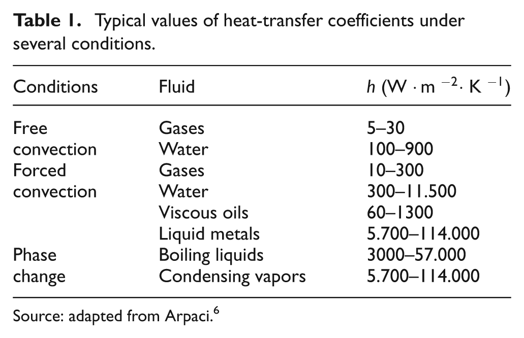
Source: adapted from Arpaci.⁶

However, the ranges for values in Table 1 are too wide for practical use in terms of measuring the effectiveness of cutting fluids applied to machining processes. Additionally, the constant appearance of new cutting fluids with compositions and additive substances of different nature makes their selection a challenging task for manufacturing engineers. In addition, new application systems, such as the minimum quantity of lubricant (MQL) system, require a greater understanding of the processes of heat conduction in the region of chip formation. Therefore, the magnitude of the heat-transfer coefficient, $h$ , becomes decisive in any attempt to model the heat-transfer problem in metal cutting operations. Not only is the study of $h$ important, but it also suggests a similar investigation into the thermal conductivity, $k$ , of the solid parts involved in this particular heat-transfer problem. Both effects, however, may be treated as a single dimensionless number by the use of the Biot number, $Bi$ , given by

Bi = \frac{hL}{k} = \frac{L / k}{1 / h}

(2)

where $L$ (m) is the characteristic length dimension of the body being studied and $k$ is the thermal conductance of the same body. The Biot number may physically be interpreted as the ratio of the internal and external conductance of a solid body being exposed to a fluid.⁶ When the internal conductance is large, $k / L \to \infty$ and $Bi \to 0$ . In such cases, this corresponds to small $L$ , or large $k$ , and the spatial temperature variation perpendicular to the face having this energy transfer can be neglected. Therefore, this case leads to an approach using a lumped system analysis.^7,8

In contrast, when the external conductance is large, which is the case in boiling, condensation and highly turbulent flows, for example, $h \to \infty$ and $Bi \to \infty$ . This implies that the body face temperature tends to ambient temperature. In this way, the general boundary conditions may be simplified to a specified boundary temperature, which is assumed to be approximately equal to the ambient temperature. When internal and external conductance are comparable, i.e. $Bi$ has a moderate value and neither of the above described conditions can be applied, the general boundary conditions cannot be simplified, and the problem must be solved in terms of this condition. This case required the distributed system approach. Therefore, the magnitude of the Biot number is decisive for the type of boundary conditions to be used in the formulation of a conduction heat-transfer problem.

Most recent studies have been working in this direction,^9,10,11,12 but have concentrated on calculating the heat-transfer coefficient of the temperature of the environment where air is the cooling fluid. Few studies have worked with different fluid nature and compositions, as well as different application systems.^13,14,15 Sales et al.¹³ calculated analytically the heat-transfer coefficient between a cylindrical bar of AISI 8640 (American Iron and Steel Institute) and five kinds of ambient fluid during a machining process (turning) with the same application system. Cirillo and Isopi¹⁴ obtained numerically the heat-transfer coefficient for nine circular confined air jets vertically impinging on a flat plate of glass. Convective heat-transfer coefficients were also estimated by Kohut et al.¹⁶ for specific conditions (air and with an impinging coolant jet) during the turning of a cylindrical workpiece using a control-volume finite difference (CFD). There have been several attempts and methods to evaluate the values of $h$ . Sales et al.,¹³ for example, applying the capacitance method, estimated $h = 113.2$ W · m⁻² · K⁻¹ and $Bi = 0.0358$ , for neat oil, in a flood system. Using an air jet on glass and CFD models, Cirillo and Isopi¹⁴ obtained values between 1.95 and 3.48 $\times 10^{2}$ W · m⁻² · K⁻¹. Causone et al.¹² measured a global heat-transfer coefficient in a room with stationary air and a radiant ceiling, and estimated values were around 1.1 and 1.3 $\times 10$ W · m⁻² · K⁻¹. Rahman and Kumar¹¹ used air blowing over drying vegetables and found the values of $h$ to be around 1.5 and 2.5 $\times$ 10 W · m⁻² · K⁻¹. Yang et al.¹⁷ used air flowing around a human body shape, and the values were around 0.5 and 2.5 $\times 10$ W · m² · K⁻¹ for an air speed between 0.2 and 1.4 m · s⁻¹. In quenching metals for heat treatment applications, water was the fluid and Al–Cu alloys were the metal bodies in the cooling process. Typical values were around 1.5 and 15 $\times$ $10^{3}$ W · m⁻² · K⁻¹. Some authors have also developed probes capable of evaluating the values of $h$ for machine tool applications.^13,16 The experimental methods vary, but the majority measure the fluid and the surface temperature, $T_{s}$ and $T_{\infty}$ , together with the total heat flux over a known area and apply equation (1), which is also the basis for the present work.

The present work aims at an experimental evaluation of the convective heat-transfer coefficient for cutting fluids normally used in machining processes. The heat source provided by the metal cutting was simulated by electrical heating of the plate. The electric heating was selected to simulate the workpiece temperature of the milling process described by Luchesi¹⁸ and Luchesi and Coelho.¹⁹ Three different cooling conditions were used: the dry cooling system, the flooded cooling system and the MQL cooling system, as well as two different cutting fluids for each of the last two systems. In addition, the present work also discusses the most appropriate mathematical approach for the heat-conduction problem by calculating the Biot number for each cooling condition tested. If the Biot number results are lower than 0.1, this indicates that less than 5% error will be present when assuming a lumped model of transient heat transfer.^9,20,21 Using the lumped approach, the model of temperature results are much more simple since the elimination of spacewise temperature variation leads to simple exponential heating equations.²¹ For moderate to large values of Biot number, however, the temperature gradients within the solid are significant.⁵ A Biot number greater than 0.1 indicates a study of transient multidimensional conduction and differential formulation for the heat-transfer problem.²²

Experiments

Experimental system

Figure 1 shows a schematic of the experimental arrangement used to obtain heat-transfer coefficients in steady state adapted from a suggested method found in Incropera and Witt.⁵

Figure 1.

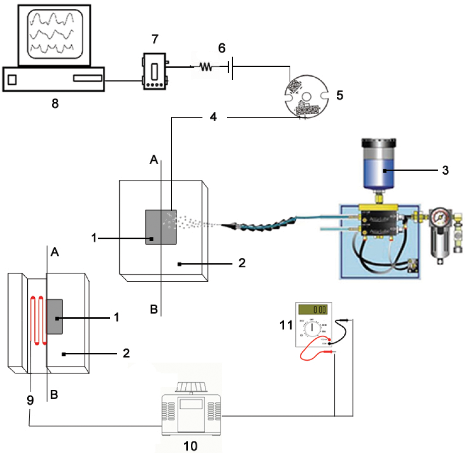
Experimental system: 1, steel plate 4340; 2, insulated box; 3, cooling system; 4, thermocouples; 5, transmitter TxBlock; 6, low-pass filter; 7, interface; 8, computer; 9, resistance; 10, adjustable resistor; 11, multimeter.

It uses a thin steel plate made of AISI 4340 with dimensions 51 $\times$ 43.8 mm with 3 mm of thickness and a thermal conductance of 44 W · m⁻² · K⁻¹, which was subjected to parallel flow of the coolant and simultaneous electrical heating in order to maintain the temperature surface $T_{s}$ greater than $T_{\infty}$ , the fluid temperature. The thin plate was totally thermoisolated, except on one flat face ( $A_{p} = 51 \times 43.8$ mm), which was subjected to the cooling system to be tested. The insulation material used was Al₂O₃ ceramic with around 20 mm of thickness. The temperatures $T_{s}$ and $T_{\infty}$ were measured by alumel–cromel thermocouples attached to an acquisition system. All the thermocouples were calibrated in a thermostat bath for the expected temperature range (between 293.15 and 368.15 K).

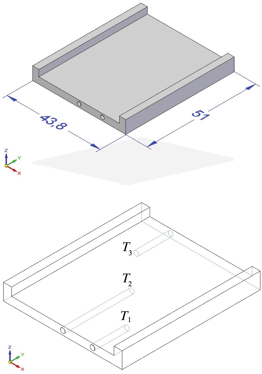
The surface temperature, $T_{s}$ , of the thin plate was measured at three points by embedded thermocouples located at $T_{1}$ , $T_{2}$ and $T_{3}$ , as shown in Figure 2. Then, $T_{s}$ was calculated by the arithmetic average of these three values. The electric heating system consisted of a Nikrothal-80 (3.7 $Ω \cdot$ m⁻¹) resistor (Figure 1, item 9) powered by a controlled voltage. The electric current was measured using a Fluke multimeter model IV series 89.

Figure 2.

Geometry of the steel plate 4340 and location of holes for insertion of thermocouples (dimensions in mm).

The total electric power supplied can be calculated as

P = E \cdot I (W)

(3)

where $E$ is the voltage (V) and $I$ is the current (A). Considering that all the electric power is converted into heat, the values of $h$ can be calculated as

h = \frac{P}{A_{p} (T_{s} - T_{\infty})}

(4)

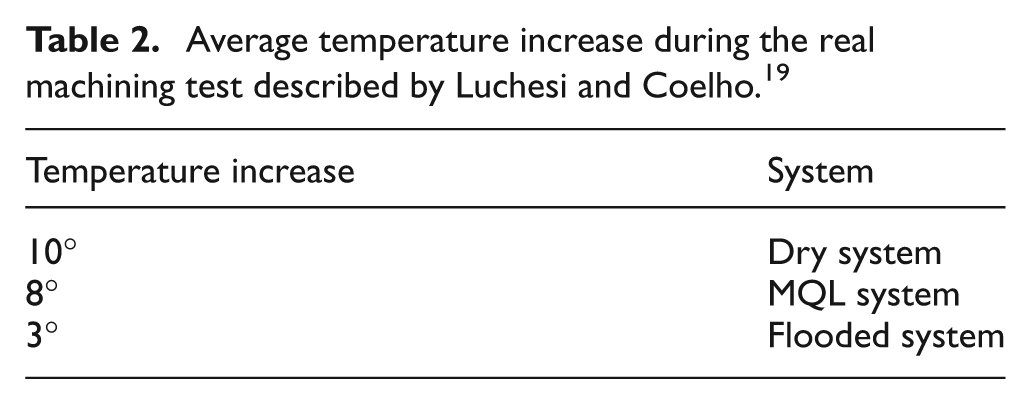
Five values of $h$ were calculated for each cooling system by varying the voltage. For each new voltage, the current was measured and the power calculated. For each change in electrical power, there was enough time for the system to reach steady conditions, in terms of surface temperature. The variation of the power was established to cover all values of average temperature increase during the real machining test described by Luchesi and Coelho.¹⁹ These values are given in Table 2.

Table 2.

Average temperature increase during the real machining test described by Luchesi and Coelho.¹⁹

Temperature increase	System
10°	Dry system
8°	MQL system
3°	Flooded system

Cutting fluid application systems

For the presented trials, two application systems were used: flooded and MQL.^23,24

The flooded system consisted of one single nozzle placed at an angle of approximately $25 \circ$ with the thin plate cooling face, and at approximately 10 mm above it and 40 mm distance in order to provide a parallel flow. The flow rate used was about 10 l/min (computer numerical control (CNC) flow rate) for all the trials, which is the normal flow rate used in machining operations.

The MQL system consisted of two nozzles placed at an angle of $45 \circ$ with the cooling face and 15 mm above it. The device was set for 15 ml/h of oil and 70 m³/h of compressed air at 0.4 MPa of pressure. The flow rate of oil, pressure and air velocity was chosen according to Diniz et al.,²⁵ Braga et al.²⁶ and Bruni et al.²⁷ Diniz et al.²⁵ showed that the amount of oil, from 10 to 60 ml/h, inside the airflow did not significantly affect the performance of the process.

Figure 3 illustrates the control unit, which sets the amount of oil and all the adjustments of the flow of compressed air.

Figure 3.

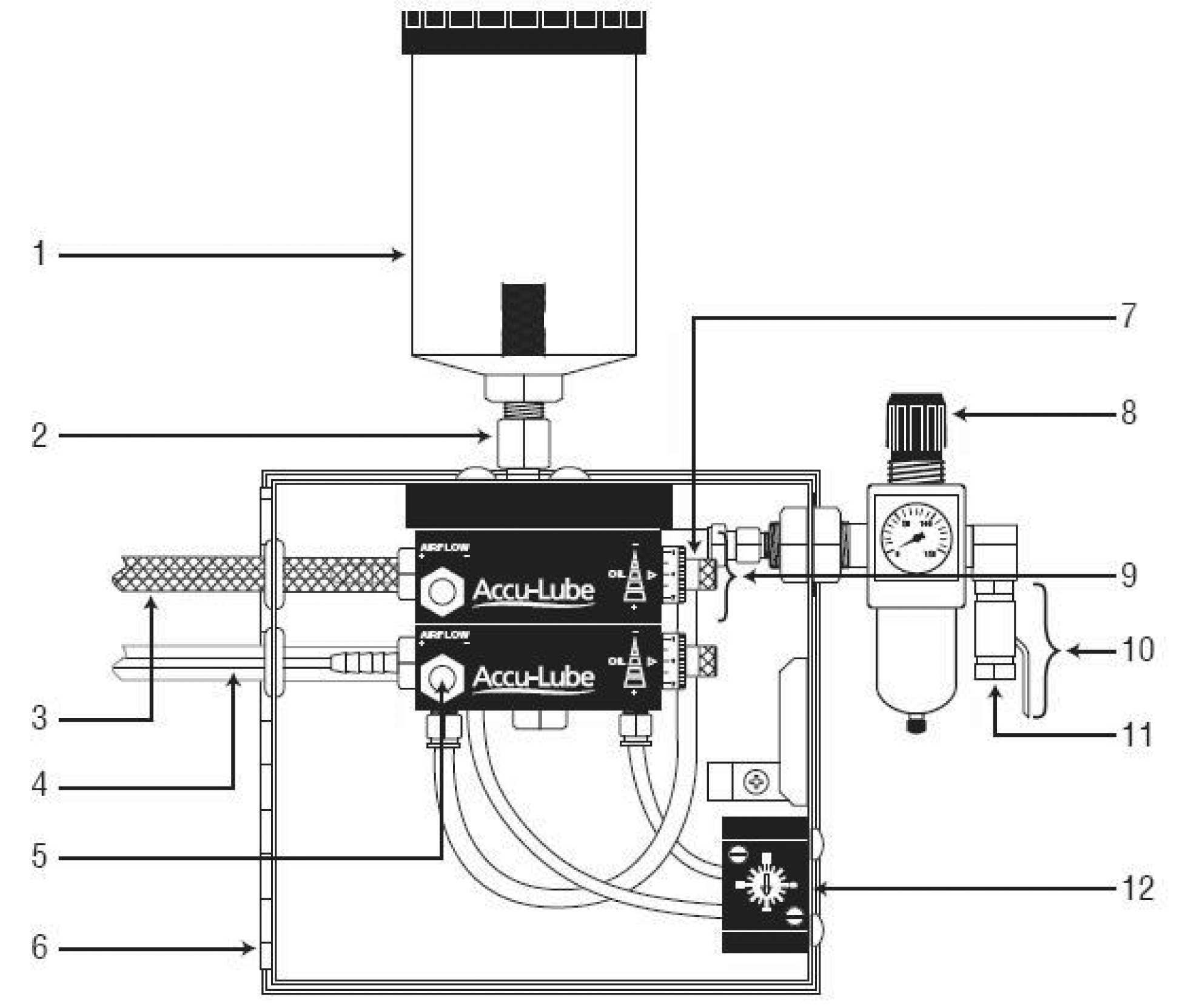
Control unit of the MQL system: 1, oil reservoir with a capacity of 300 ml; 2, connector; 3, output for the wand air; 4, nozzle; 5, valve controlling the flow of air; 6, metal box; 7, control of the fluid inlet; 8, air filter and manometer; 9, pressure pump; 10, manual control valve (on/off); 11, air inlet; 12, regulator frequency drop of fluid.

Fluids

Two fluids were used with the MQL system, as well as with the flooded system, according to the characteristics shown in Table 3.

Table 3.

Fluid properties.

Fluid	Viscosity at 313.15K (m ² · s ⁻¹)	Density at 293.15K (kg · m ⁻³)	Vegetable or mineral portion
MQL 1	0.000018	920	100% mineral
MQL 2	0.000022	900	83% vegetable
Fluid 1	0.000059	950	59% mineral
Fluid 2	0.000056	950	45% vegetable

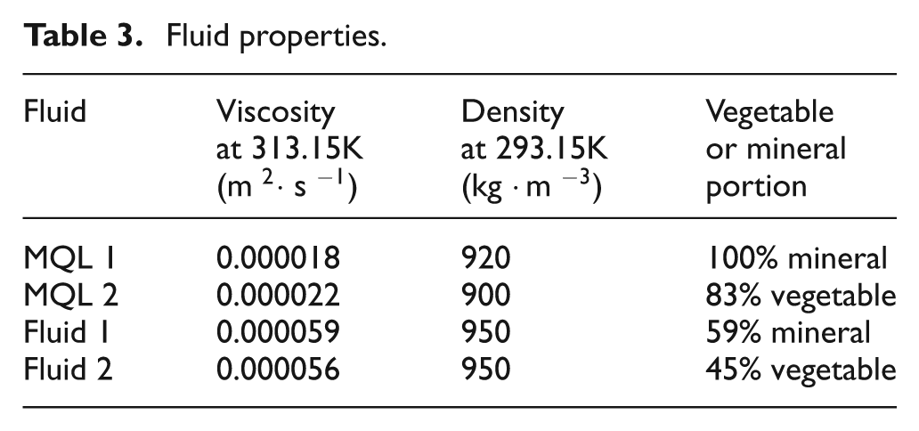
The two fluids in the MQL system are utilized with a flow rate of 15 ml/h and an air pressure of 0.4 MPa.

Results

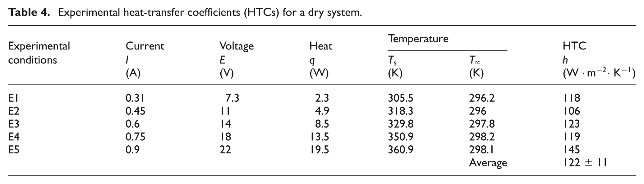
The heat-transfer coefficient was calculated using equation (1). Tables 4 to 8 show the electric measured values for the dry, flooded and MQL systems. These data were used as input data to calculate the convective transfer coefficient $h$ for each cooling system. The tables also show the averages and 95% confidence interval for the five values, assuming $h$ should be a constant value.

Table 4.

Experimental heat-transfer coefficients (HTCs) for a dry system.

Experimental	Current	Voltage	Heat	Temperature		HTC
conditions	$I$	$E$	$q$	$T_{s}$	$T_{\infty}$	$h$
	(A)	(V)	(W)	(K)	(K)	(W · m⁻² K⁻¹)
E1	0.31	7.3	2.3	305.5	296.2	118
E2	0.45	11	4.9	318.3	296	106
E3	0.6	14	8.5	329.8	297.8	123
E4	0.75	18	13.5	350.9	298.2	119
E5	0.9	22	19.5	360.9	298.1	145
					Average	122 $\pm$ 11

Table 5.

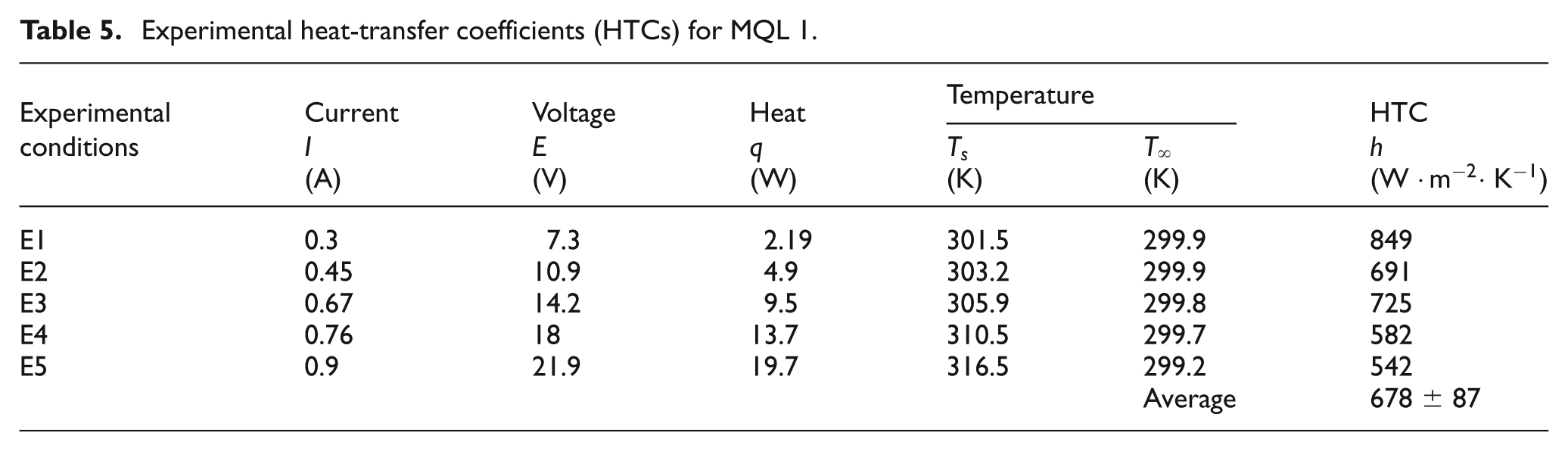
Experimental heat-transfer coefficients (HTCs) for MQL 1.

Experimental	Current	Voltage	Heat	Temperature		HTC
conditions	$I$	$E$	$q$	$T_{s}$	$T_{\infty}$	$h$
	(A)	(V)	(W)	(K)	(K)	(W · m⁻² · K⁻¹)
E1	0.3	7.3	2.19	301.5	299.9	849
E2	0.45	10.9	4.9	303.2	299.9	691
E3	0.67	14.2	9.5	305.9	299.8	725
E4	0.76	18	13.7	310.5	299.7	582
E5	0.9	21.9	19.7	316.5	299.2	542
					Average	678 $\pm$ 87

Table 6.

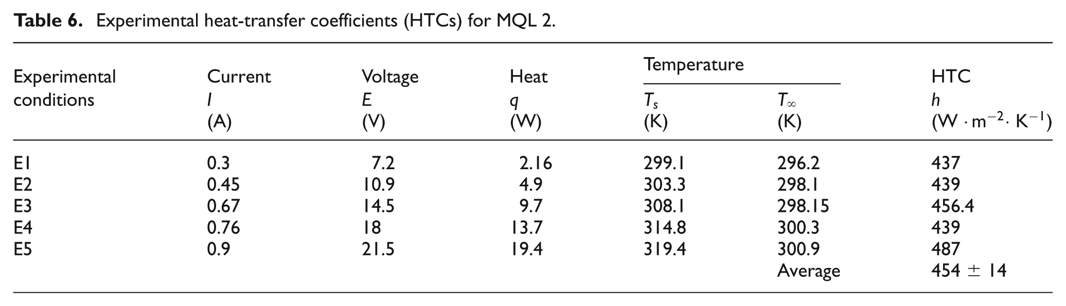
Experimental heat-transfer coefficients (HTCs) for MQL 2.

Experimental	Current	Voltage	Heat	Temperature		HTC
conditions	$I$	$E$	$q$	$T_{s}$	$T_{\infty}$	$h$
	(A)	(V)	(W)	(K)	(K)	(W · m⁻² · K⁻¹)
E1	0.3	7.2	2.16	299.1	296.2	437
E2	0.45	10.9	4.9	303.3	298.1	439
E3	0.67	14.5	9.7	308.1	298.15	456.4
E4	0.76	18	13.7	314.8	300.3	439
E5	0.9	21.5	19.4	319.4	300.9	487
					Average	454 $\pm$ 14

Table 7.

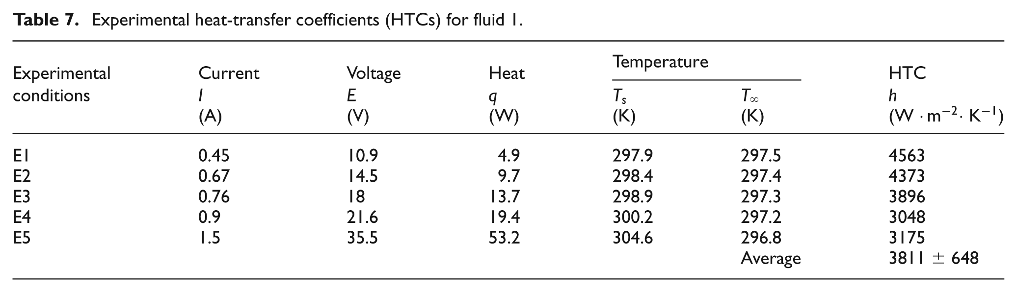
Experimental heat-transfer coefficients (HTCs) for fluid 1.

Experimental	Current	Voltage	Heat	Temperature		HTC
conditions	$I$	$E$	$q$	$T_{s}$	$T_{\infty}$	$h$
	(A)	(V)	(W)	(K)	(K)	(W · m⁻² · K⁻¹)
E1	0.45	10.9	4.9	297.9	297.5	4563
E2	0.67	14.5	9.7	298.4	297.4	4373
E3	0.76	18	13.7	298.9	297.3	3896
E4	0.9	21.6	19.4	300.2	297.2	3048
E5	1.5	35.5	53.2	304.6	296.8	3175
					Average	3811 $\pm$ 648

Table 8.

Experimental heat-transfer coefficients (HTCs) for fluid 2.

Experimental	Current	Voltage	Heat	Temperature		HTC
conditions	$I$	$E$	$q$	$T_{s}$	$T_{\infty}$	$h$
	(A)	(V)	(W)	(K)	(K)	(W · m⁻² · K⁻¹)
E1	0.45	10.9	4.9	298.8	298.5	6844
E2	0.67	14.5	9.7	299.6	298.9	6455
E3	0.76	18	13.7	299.9	298.8	5614
E4	0.9	21.5	19.35	301.1	298.6	3553
E5	1.5	36.5	54.7	304.9	298.8	4085
					Average	5310 $\pm$ 1034

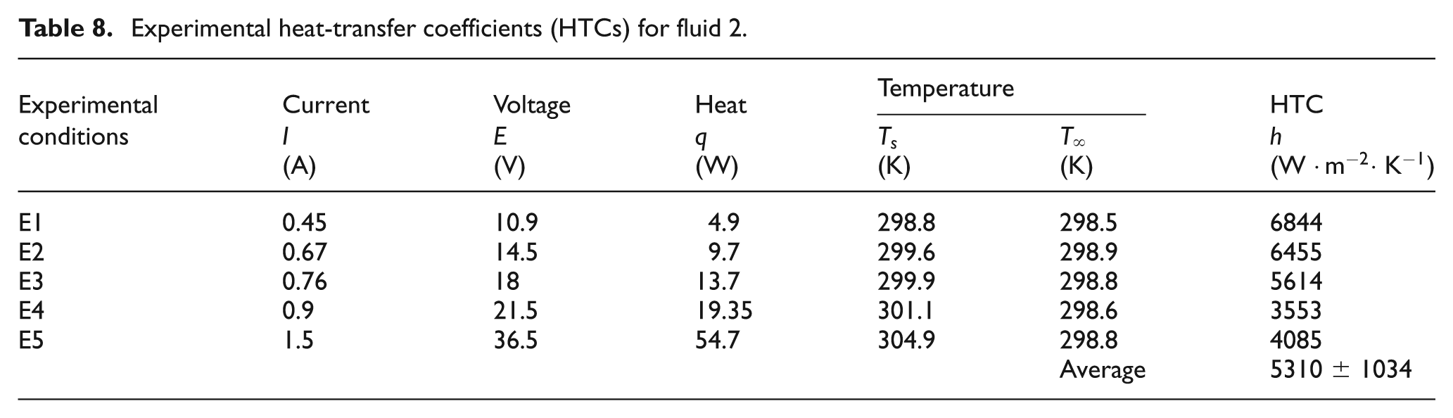
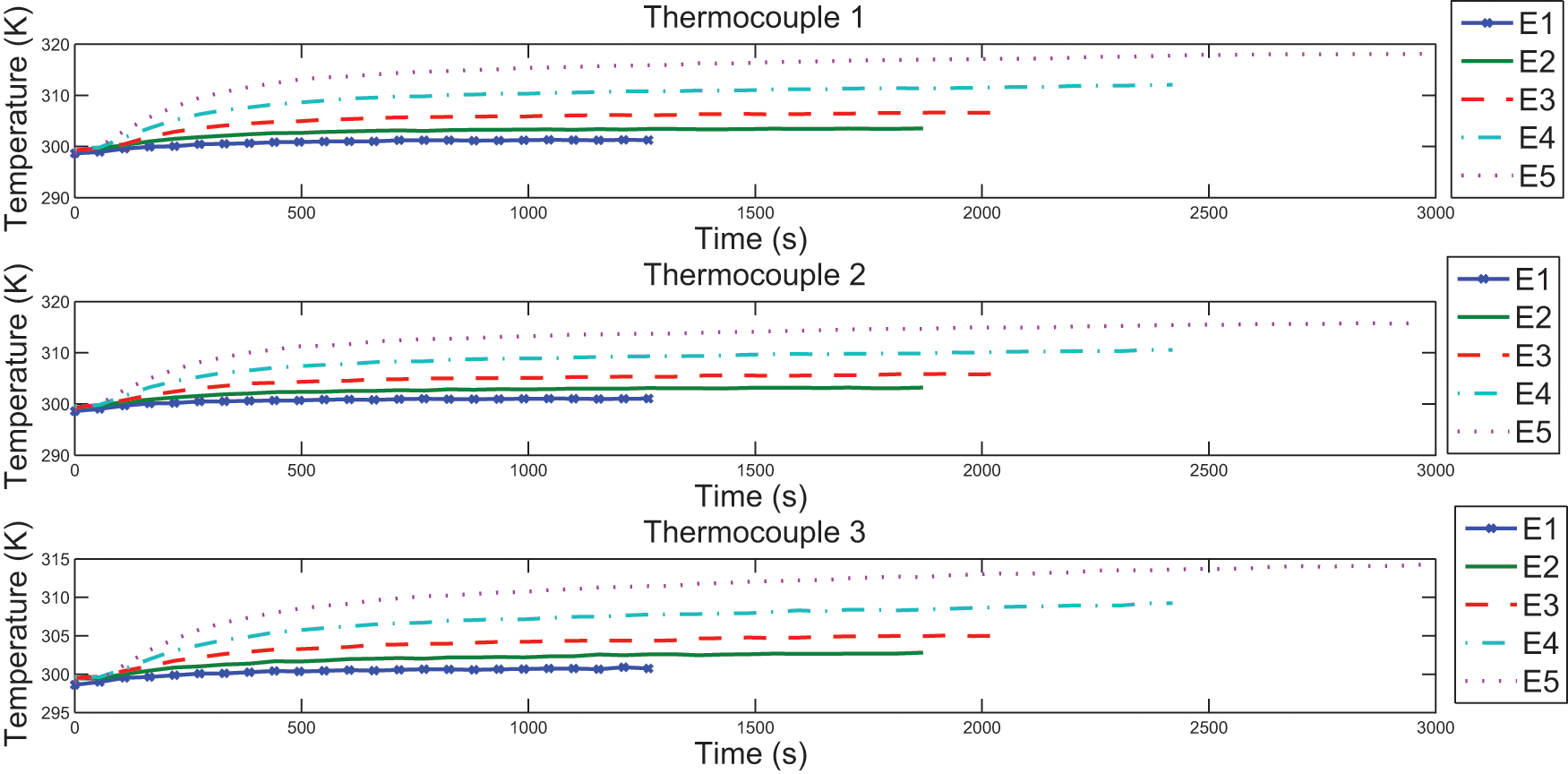
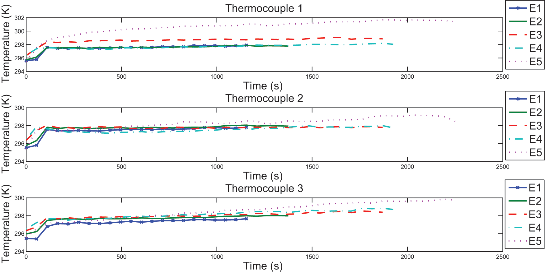
Figure 4 shows the temperature versus time measured for experimental conditions E1 to E5 with the dry system. For each test, E1 to E5, five tests were performed, in which the temperature of the thermocouples was measured until the temperature remained steady, i.e. the temperature for the end time from the graphs in Figure 4. 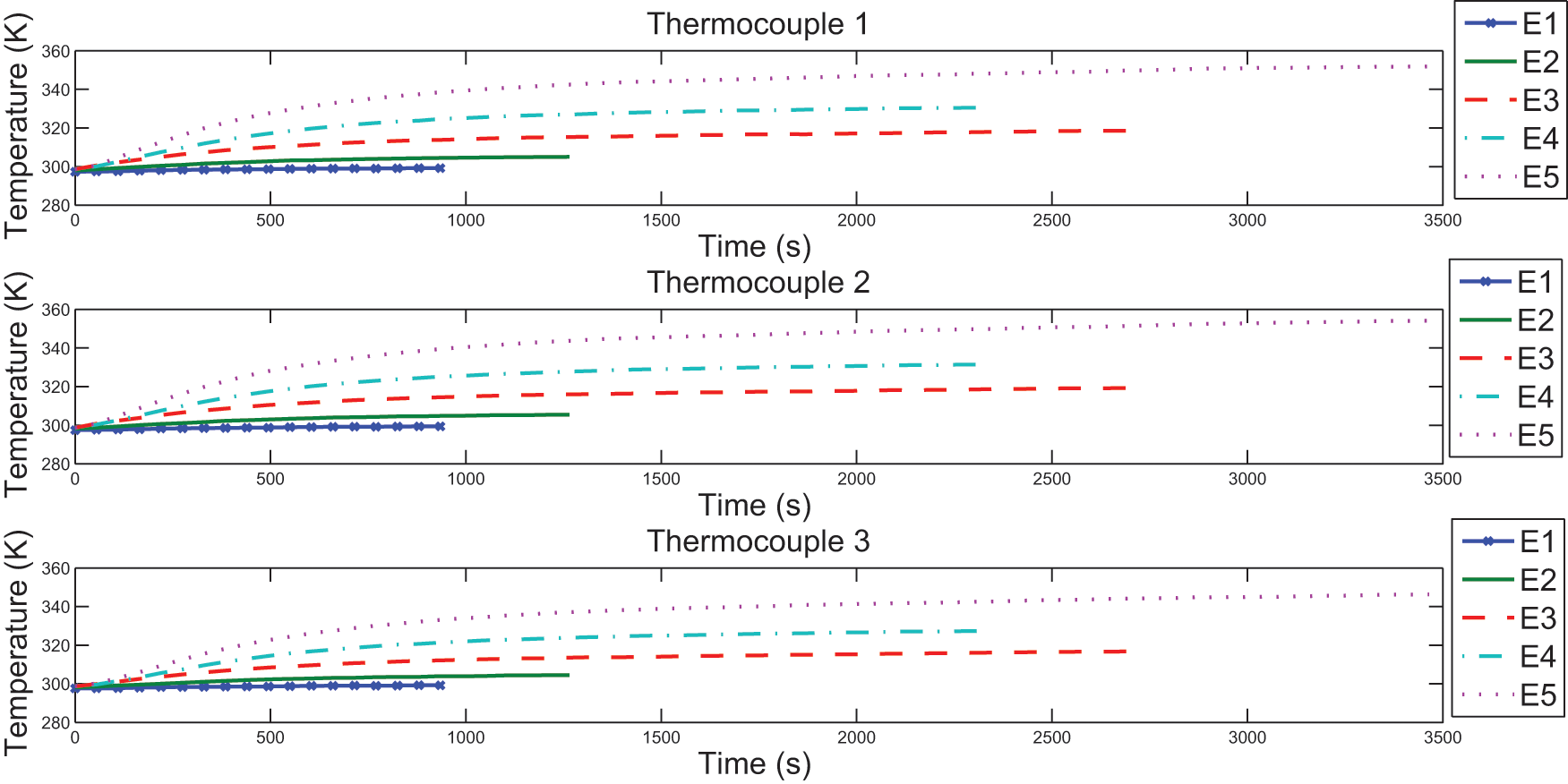From these results, the average temperature stability was calculated for each thermocouple $T_{1}$ , $T_{2}$ and $T_{3}$ , then the surface temperature $T_{s}$ , Table 4, was calculated as the average of these values. The same procedure was used to calculate the surface temperature $T_{s}$ for the MQL system (Tables 5 and 6; and Figures 6 and 7) and the flooded system (Tables 7 and 8; and Figures 9 and 10).

Figure 4.

Temperatures measured for experimental conditions E1 to E5 with the dry system.

Figure 5.

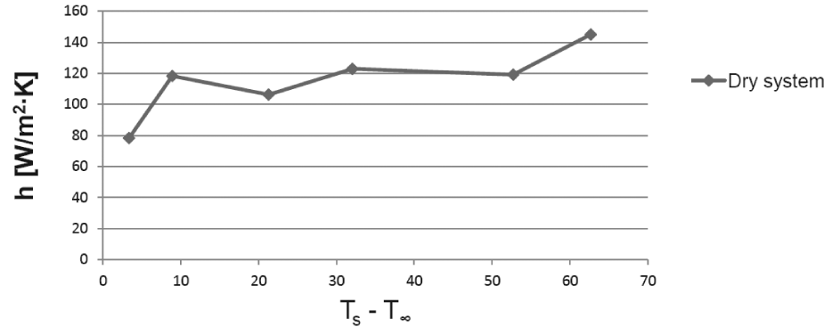
Graph of heat-transfer coefficient versus temperature difference $T_{s} - T_{\infty}$ for the dry system.

Figure 6.

Temperatures measured for experimental conditions E1 to E5 with the MQL 1 system.

Figure 7.

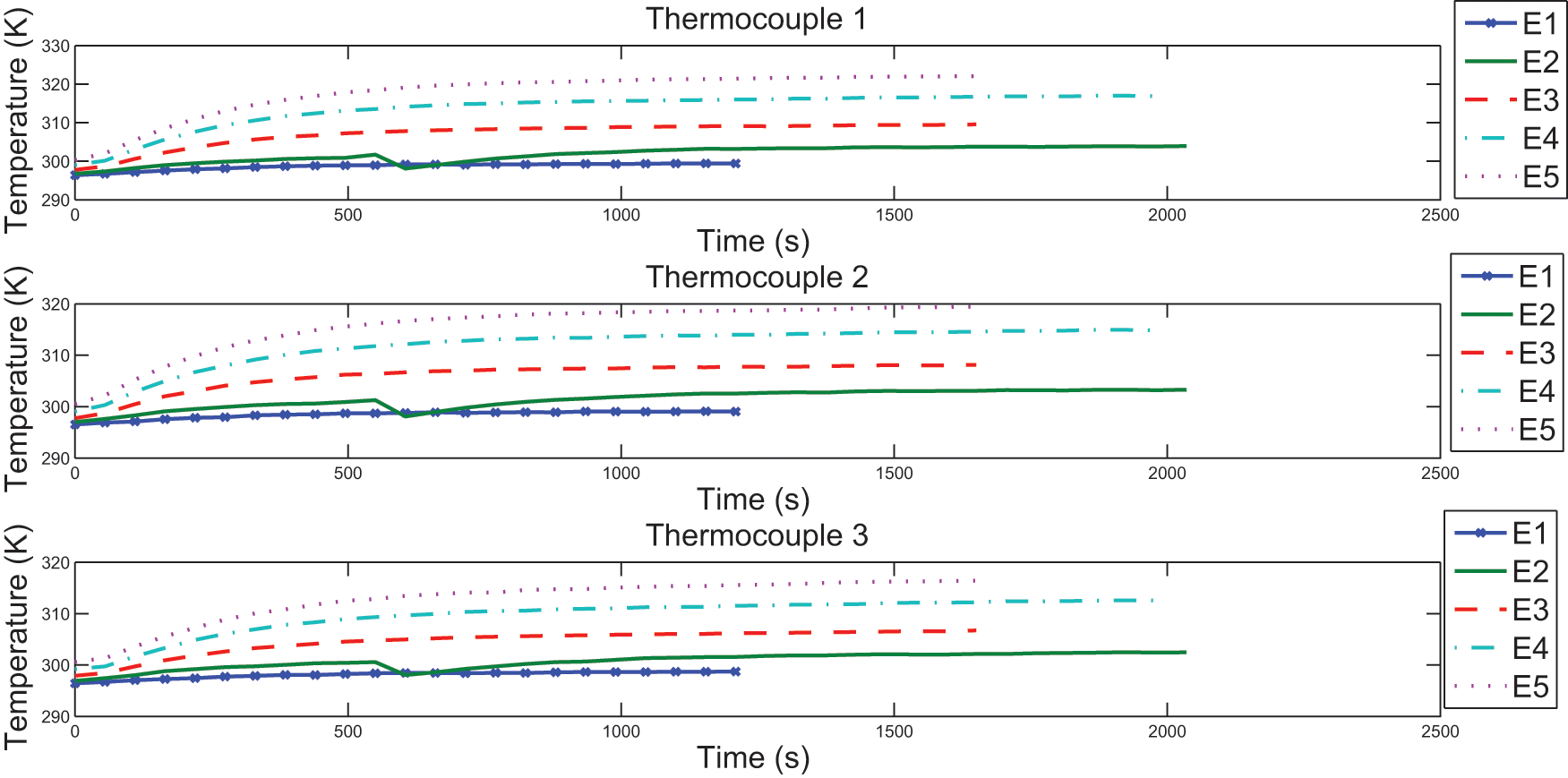
Temperatures measured for experimental conditions E1 to E5 with the MQL 2 system.

Figure 8.

Graph of heat-transfer coefficient versus temperature difference $T_{s} - T_{\infty}$ for the MQL system.

Figure 9.

Temperatures measured for experimental conditions E1 to E5 with the fluid 1 system.

Figure 10.

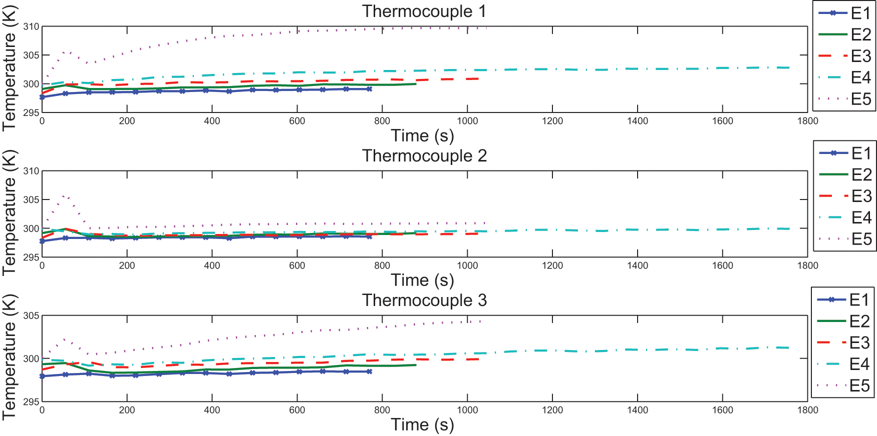
Temperatures measured for experimental conditions E1 to E5 with the fluid 2 system.

Using equation (2), and the values from Table 3, the average heat-transfer coefficient, together with the value of $k$ for AISI 4340 ( $k = 44$ W · m⁻¹ · K⁻¹), one obtains $Bi = 0.0083 \pm 0.0006$ for the dry condition. Such a value indicates that a spatially lumped instantaneous temperature for the solid is the most adequate one for this cooling system. This can offer a series of advantages, such as uniform distribution ( $T (x, t) \approx T (t)$ ) when estimating the temperature distribution on the chip formation region.

Figure 5 shows the behavior of the curve for the heat-transfer coefficient versus the temperature difference for a dry system.

It can be noticed from Figure 5 that $h$ tends to slightly increase with increasing body surface temperature, which is expected, since the heat, in this case, is predominantly transmitted by conduction.

Table 5 shows the corresponding experimental data related to the heat-transfer coefficient for the MQL 1 system. For the MQL 1 system, the Biot number was $Bi = 0.046 \pm 0.006$ . As stated above, the Biot number also allows the use of the lumped approach when using MQL 1, as for the dry system.

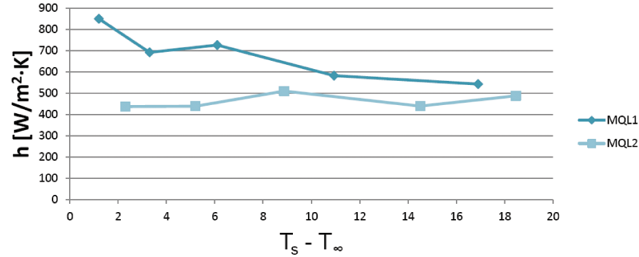
Table 6 shows the experimental heat-transfer coefficients for the MQL 2 system and equivalent data. The Biot number resulted in $Bi = 0.032 \pm 0.002$ for the MQL 2 system and lumped capacity analysis can also be applied.²¹

Figure 8 shows the behavior of the curve of the heat-transfer coefficient versus the temperature difference for the MQL system.

Compared to the dry system above, the use of MQL systems significantly increases $h$ value by about 5 to 6 times, although for the same internal conductance ( $k / L$ ), the Biot numbers were still lower than 0.1. Using MQL 1, the $h$ value decreases as surface temperature increases, while with MQL 2, there is less change. Such data indicate that the mineral oil used in MQL 1 became less efficient in the cooling effect as the surface temperature increased, and the vegetable-based fluid seemed to be less sensitive to those changes. It can be stated that if the machining process results in higher temperatures on the body surface, the fluids will behave very similarly. However, for low-temperature processes, such as tapping, broaching, etc., the best choice would be MQL 1.

Table 7 shows the experimental heat-transfer coefficients and data for the flooded system using fluid 1. The Biot number was $Bi = 0.259 \pm 0.038$ , which is well above the established threshold value for lumped analysis ( $Bi \leq 0.1$ ).

Table 8 shows similar values for the flooded system with fluid 2, which resulted in a Biot number of $Bi = 0.362 \pm 0.081$ , equally above the threshold for lumped analysis ( $Bi \leq 0.1$ ).

Figure 11 shows the behavior of the curve of the heat-transfer coefficient versus the temperature difference for the flooded system.

Figure 11.

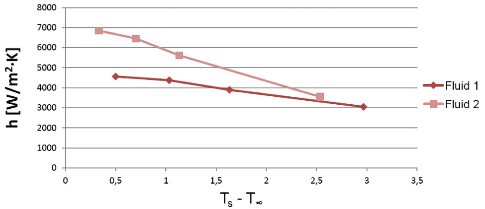
Graph of heat-transfer coefficient versus temperature difference $T_{s} - T_{\infty}$ for the flood system.

With the flooded system, lumped analysis is inappropriate and multidimensional analyses must be used. The mathematical models for temperature distribution and heat propagation will certainly be much more complex, as will the solutions, judging by the Biot number found. When comparing the $h$ values with the others found so far for MQL and dry conditions, the efficiency of the flooded cooling system was much higher, as expected. Comparing both fluids used in the flooded system, the vegetable-based one is much more efficient at low temperatures, although both tend to lose efficiency rapidly. In general, both cooling systems tested tend to lose efficiency (lower $h$ values) as the surface temperature increases and the most efficient was the flooded one. There can be differences in efficiency according to the type of oil used in both systems, depending on the surface temperature. For machining processes where low-temperature surfaces are expected, the differences in heat-transfer coefficients can be significant, although above certain values, all the oils used tend to yield similar $h$ values.

Conclusion

According to the results found in the present work, some initial conclusions can be drawn.

For dry systems, MQL 1 and MQL 2, the lumped approach for theoretical analysis is expected to yield reasonable estimates because the Biot number was found to be lower than 0.1. This magnitude of the Biot number for these systems shows that the body internal heat conductance is much higher than the heat convection away from its surface. With materials different from AISI 4340, the results can be different because the Biot number depends on the material thermal conductivity.

When dealing with machining processes in which the Biot number is less than 0.1, as with the dry and MQL systems in the present work, a lumped and much more simple model for temperature distribution and heat propagation can be used to describe the phenomenon. In these cases, the cooling system represents the highest barrier for the heat to flow away from the workpiece. In addition, it can be stated that the inefficiency of the cooling system, compared to the heat conduction of the solid body itself, becomes the most difficult parameter to remove heat from the workpiece.

When comparing both fluids used in the MQL systems, the mineral-based one was more efficient at low temperature differences, although for higher differences, both tend to converge to an average of about 500 W · m⁻² · K⁻¹. For a dry system, the $h$ value tends to increase with temperature difference, but also seems to converge to around 122 W · m⁻² · K⁻¹.

For both flooded systems hereby tested, the Biot number was higher than 0.1, so more complicated heat-transfer equations for transient heat conduction are required to describe the time-varying and non-spatially-uniform temperature field within the solid body. In contrast, the cooling system imposes less resistance for the heat to flow away from the workpiece compared to the internal resistance of the solid body.

When the Biot number is higher than 0.1, as in the case for both flooded systems tested in the present work, the cooling system makes it easy for the heat to flow away from the workpiece by imposing less resistance.

When comparing both fluids used for the flooded system, the vegetable-based one seems to have a slightly better cooling effect than the mineral-based one, but only at low temperature differences. Because the flooded system is so efficient in cooling, the surface temperature could not reach higher values.

Footnotes

Acknowledgements

We would like to thank the Blaser Swisslube of Brazil for providing the cutting fluids tested.

Funding

This work was supported by FAPESP Process 2007/00338-0.

References

Jung

. Environmentally conscious hard turning of cemented carbide materials on the basis of micro-cutting in SEM (2nd report). J Mech Sci Technol 2009; 23: 1959–1966.

Abdalla

Baines

McIntyre

. Development of novel sustainable neat-oil metal working fluids for stainless steel and titanium alloy machining. Int J Adv Manufact Technol 2009; 23: 1959–1966.

Atmadi

Stephenson

Liang

. Cutting fluid aerosol from splash in turning. Int J Adv Manufact Technol 2001; 17: 238–243.

Machado

Coelho

Abrão

. Teoria da usinagem dos materiais [Machining theory of materials] 1st ed. Rio de Janeiro: Edgard Blücher, 2009.

Incropera

Witt

. Fundamentals of heat and mass transfer 3rd ed. New York: John Wiley & Sons, 1990.

Arpaci

. Conduction heat transfer Massachusetts: Addison-Wesley Publishing Company, 1966.

Cortes

Campo

Arauzo

. Reflections on lumped models of unsteady heat conduction in simple bodies. Int J Thermal Sci 2003; 42: 921–930.

Lienhard

JHI

Lienhard

JHV

. A heat transfer textbook 3rd ed. Cambridge: Phlogiston Press, 2008.

Cancillo

Morales

Gallego

. An approximated method of calculating the heat transfer coefficient in metal bars. J Eng Phys Thermophys 2000; 73(6): 1323–1331.

10.

Heidrich

Wolfersdorf

Schmidt

. Estimation of internal heat transfer coefficients and detection of rib positions in gas turbine blades from transient surface temperature measurements. J Phys: Conf Ser– 6th International Conference on Inverse Problems in Engineering: Theory and Practice 2008; 135: 1–8.

11.

Rahman

Kumar

. Evaluation of convective heat transfer coefficient during drying of shrinking bodies. Energy Conv Manage 2006; 471: 2591–2601.

12.

Causone

Corgnati

Filippi

. Experimental evaluation of heat transfer coefficients between radiant ceiling and room. Energy Buildings 2009; 41: 622–628.

13.

Sales

Guimarães

Machado

. Cooling ability of cutting fluids and measurement of the chip-tool interface temperatures. Ind Lub Tribol 2002; 54(2): 57–68.

14.

Cirillo

Isopi

. Glass tempering heat transfer coefficient evaluation and air jets parameter optimization. App Thermal Eng 2009; 29: 1173–1179.

15.

Khaled

ARA

. Conduction heat and entropy transfer in a semi-infinite medium and wall with a combined periodic heat flux and convective boundary condition. Int J Thermal Sci 2008; 47: 76–83.

16.

Kohút

Horejs

Mares

. Experimental identification of convective heat transfer in machine tools. In: Proceedings of the World Congress on Engineering 2011 WCE, 2011, London, UK, vol 3, pp 1–4;.

17.

Yang

Kato

Seo

. Evaluation of the convective heat transfer coefficient of the human body using the wind tunnel and thermal manikin. J Asian Archit Building Eng 2009; 8: 563–569.

18.

Luchesi

. Estudo Teòrico da Condução de Calor e Desenvolvimento de um Sistema para a Avaliação de Fluidos de Corte em Usinagem (Theoretical study of heat conduction and Development of a System for the Evaluation of Cutting Fluids in Machining) PhD Thesis, University of Sao Paulo, 2011.

19.

Luchesi

Coelho

. An inverse method to estimate the moving heat source in machining process. App Thermal Eng 2011; p.1–11. Accepted.

20.

Özisik

. Heat transfer New York: McGraw-Hill, 1985.

21.

Sha

Gani

. Transient heat conduction at low Biot numbers. Lett Heat Mass Transf 1981; 8: 379–395.

22.

Arpaci

Selamet

Kao

. Introduction to heat transfer New Jersey: Prentice Hall, 2000.

23.

Kalpakjian

. Manufacturing processes for engineering materials 2nd ed. New York: Addison-Wesley, 1991.

24.

Boothroyd

Knight

. Fundamentals machining and machine tools 2nd ed. New York: Marcel Dekker, 1989.

25.

Diniz

Ferreira

Filho

. Influence of refrigeration/lubrication condition on (SAE 52100) hardened steel turning at several cutting speeds. Int J Machine Tools Manufact 2003; 43: 317–326.

26.

Braga

Diniz

Miranda

GWA

. Using a minimum quantity of lubricant (MQL) and a diamond coated tool in the drilling of aluminum–silicon alloys. J Mater Process Technol 2002; 122: 127–138.

27.

Bruni

Forcellese

Gabrielli

. Effect of the lubrication-cooling technique, insert technology and machine bed material on the workpart surface finish and tool wear in finish turning of AISI 420B. Int J Machine Tools Manufact 2006; 46: 1547–1554.

28.

ITW ROCOL. Accu–Lube–Precision Pump Applicator, User’s manual—installation and operating instructions Illinois: ITW ROCOL, 2009.

Experimental investigations of heat transfer coefficients of cutting fluids in metal cutting processes: analysis of workpiece phenomena in a given case study