Multi-objective multi-parameter optimization of the industrial LBW process using a new optimization algorithm

Abstract

The concept of automation has been brought into the industries in order to increase the production rate and at the same time to minimize the production cost. The LBW process is widely replacing manual welding processes in many fabrication industries owing to the high level of automation. In the present work, an attempt is made to achieve conflicting objectives by finding optimum parameter settings for the LBW process. A recently developed advanced optimization algorithm is applied for parameter optimization of the LBW process. Two different multi-objective optimization examples are considered and significant improvement is obtained by the proposed optimization algorithm as compared with the earlier works.

Introduction

Many fabrication industries are shifting towards the automation of welding processes and there is an increasing demand for high technology processes in various fabrication industries like aerospace, defense/military, petrochemical refining, etc. Laser beam welding (LBW) is a high energy beam process that continues to expand into modern industries and new applications because of its many advantages, like close control over parameters, deep weld penetration and minimum heat inputs.

The various input parameters involved in LBW are base metal thickness, laser power, welding speed, defocusing distance, type of shielding gas combinations, torch angle, travel speed, gas flow rate and nozzle stand-off distance on the bead profile. Each input parameter plays a very significant role on output parameters like bead profile, weld joint strength, production rate, operating cost, etc. For example, decreasing the laser power may help manufacturers to save costs, but the decrease in laser power will lead to a lower fusion rate and lower production rate. Hence, optimum parameter setting of these input parameters is very important in order to satisfy all the objectives.

It is observed that various researchers have developed mathematical models for the LBW process and attempted parameter optimization by using various techniques. El-Batahgy ¹ analyzed the fusion zone shape and solidification structure by considering various parameters of the LBW process, such as base metal thickness, laser power, welding speed, defocusing distance and the type of shielding gas combinations. The commercial austenitic stainless steels such as 304L, 316L and 347 were used for the experimentation purpose. Fine microstructure was obtained with appropriate setting of welding speed and laser power. Ancona et al. ² carried out a comparative study of the influence of two different shielding gas delivery systems on an autogenous LBW process. The effects of variation of main process parameters, i.e. travel speed, beam focus position, gas flow rate and nozzle stand-off distance on the bead profile, were investigated. It was concluded that the travel speed had a significant role on the bead profile in the LBW process and the gas flow rate, and the nozzle stand-off distance had a negligible effect on the penetration depth.

Benyounis et al. ³ investigated the effect of laser welding parameters on the heat input and weld–bead profile using response surface methodology. The outcome of the work suggested that regression equations can be used to find optimum welding conditions for the desired criteria. Olabi et al ⁴ used a back propagation artificial neural network (ANN) and the Taguchi approach to find out the optimum levels of welding speed, laser power and focal position for laser welding a medium carbon steel butt weld.

Casalino ⁵ investigated the innovative arc-laser welding process by means of a regression model and full factorial experiment. A statistical-based experimental analysis technique was used to improve the result. The technique had given the analysis of effect of various process parameters on penetration. It was reported that weld penetration was affected by laser power and focus height. A deep penetration was observed with higher values of laser power and focus height. Canyurt et al. ⁶ used a stochastic search process based on a genetic algorithm approach to predict laser hybrid welded joint strength. The laser welding strength estimation model was developed to estimate the mechanical properties of the welded joint for alloy materials and the effects of six welding design parameters was examined. The work had suggested a set of optimum process parameters to achieve the desired weld joint with better quality and maximum tensile strength. Anawa and Olabi ⁷ used the Taguchi approach for developing mathematical models and for optimizing the selected welding parameters. Influence of various process parameters, like laser power, welding speed and defocusing distance on the fusion zone area, was described. It was concluded that the welding speed had a very significant effect on the fusion zone area. Park and Rhee ⁸ proposed a neural network model for predicting the tensile strength. Experimentations were carried out on the aluminium alloy and then a genetic algorithm was used to optimize the laser power, welding speed, and wire feed rate to achieve the desired weldability and productivity.

Benyounis et al. ⁹ investigated the tensile strength and impact strength along with the joint-operating cost of laser-welded butt joints made of AISI304. The important input parameters considered were laser power, welding speed and focus point position. The mathematical model was developed and the relationships between the laser welding parameters and the three responses were established. Ghosal and Chaki ¹⁰ used an ANN-optimization hybrid model to optimize depth of penetration in the LBW process. The various input welding parameters considered were laser power, focal distance from the work surface, torch angle, and the distance between the laser and the welding torch. The work showed that the ANN model developed by the authors performed better as compared with the regression model for the same output.

Padmanaban and Balasubramanian ¹¹ developed an empirical relationship to predict the tensile strength of a magnesium alloy used for LBW. The experiments were conducted based on a three-factor, three-level, central composite face-centered design matrix with full replication technique. Use of response surface methodology was made along with the design expert statistical software to optimize the results. Welding speed was found to affect the tensile strength to a significant extent. Sathiya et al. ¹² carried out experimental investigation of tensile strength and bead profiles for laser-welded butt joints. During LBW experimentation, several shielding gases were used, such as argon, helium and nitrogen. The Taguchi approach, grey relational analysis and the desirability approach were used for the optimization purpose. The authors had given a set of optimal welding parameters for each shielding gas and showed the effect of various parameters on different shielding gases.

It is observed from literature that, even though various researchers tried to achieve the optimum parameter setting for the given conditions by considering various parameters, in such works the use of any kind of advanced optimization techniques was not found. Although few algorithms, like ANN^4,10 and genetic algorithm^6,8 had been reported in literature, but those were applied only for optimization of a few parameters of the LBW process and multi-objectives were not considered. Therefore, efforts are made here to use an advanced optimization technique recently proposed by Rao et al.^13,14 for the multi-objective multi-parameter optimization of the LBW process. The detailed algorithm is explained in the next section.

Teaching–learning-based optimization algorithm

Teaching–learning-based optimization (TLBO) algorithm is a teaching–learning process inspired algorithm recently proposed by Rao et al.^13,14 based on the effect of influence of a teacher on the output of learners in a class. The algorithm mimics the teaching ability of a teacher and the learning ability of learners in a classroom. Teacher and learners are the two vital components of the algorithm and describes two basic modes of learning, through teacher (known as teacher phase) and interacting with the other learners (known as learner phase). The output of the TLBO algorithm is considered in terms of results or grades of the learners, which depends on the quality of teacher. A high-quality teacher is usually considered as a highly learned person who trains learners so that they can have better results in terms of their marks or grades. Moreover, learners also learn from the interaction among themselves, which also helps in improving their results.

A group of learners is considered as population in the TLBO algorithm and different subjects offered to the learners are considered as different design parameters and a learner’s result is analogous to the ‘fitness’ value of the optimization problem. The best solution in the entire population is considered as the teacher. The design parameters are actually the parameters involved in the objective function of the given optimization problem and the best solution is the best value of the objective function. The working of the TLBO algorithm is divided into two parts, ‘teacher phase’ and ‘learner phase’. Working of both these phases is explained below.

Teacher phase

It is the first part of the algorithm where learners learn through the teacher. During this phase a teacher tries to increase the mean result of the class in the subject taught by him or her depending on his or her capability. At any iteration i, assume that there are ‘m’ number of subjects (i.e. design parameters), ‘n’ number of learners (i.e. population size, k = 1, 2, . . ., n) and M_j,i the mean result of the learners in a particular subject ‘j’ (j = 1, 2, . . ., m). The best overall result X_{total-kbest,i}, obtained in the entire population of learners considering all the subjects together can be considered as the result of best learner k_best. However, as the teacher is usually considered as a highly learned person who trains learners so that they can have better results, the best learner identified is considered as the teacher. The difference between the existing mean result of each subject and the corresponding result of the teacher for each subject is given by

$$\text{Difference}\_\text{Mea}{\text{n}}_{\text{j},\text{k},\text{I}}={\text{r}}_{\text{i}}({\text{X}}_{\text{j},\text{kbest},\text{I}}-{\text{T}}_{\text{F}}{\text{M}}_{\text{j},\text{i}})$$

(1)

where, X_j,kbest,i is the result of the best learner (i.e. teacher) in subject j, T_F is the teaching factor that decides the value of mean to be changed, and r_i is the random number in the range [0, 1]. The value of T_F is decided randomly with equal probability as

$${\text{T}}_{\text{F}}=\text{round}[1+\text{rand}(0,1)\{2-1\}]$$

(2)

T_F is not a parameter of the TLBO algorithm. The value of T_F is not given as an input to the algorithm and its value is randomly decided by the algorithm using equation (2). After conducting a number of experiments on many benchmark functions it is concluded that the algorithm performs better if its value is between 1 and 2. However, the algorithm is found to perform much better if the value of T_F is either 1 or 2 and hence to simplify the algorithm, the teaching factor is suggested to take either 1 or 2 depending on the rounding-up criteria given by equation (2). However, one can take any value of T_F between 1 and 2.

Based on the Difference_Mean_j,k,i the existing solution is updated in the teacher phase according to the following expression

$${\text{X}\prime }_{\text{j},\text{k},\text{I}}={\text{X}}_{\text{j},\text{k},\text{I}}+\text{Difference}\_\text{Mea}{\text{n}}_{\text{j},\text{k},\text{i}}$$

(3)

where X′_j,k,i is the updated value of X_j,k,i. Accept X′_j,k,i if it gives a better function value. All the accepted function values at the end of teacher phase are maintained and these values become input to the learner phase.

Learner phase

It is the second part of the algorithm where learners increase their knowledge by interaction among themselves. A learner learns new things if the other learner has more knowledge than him or her. Considering a population size of ‘n’, the learning phenomenon of this phase is expressed below.

Randomly select two learners, P and Q, such that X′_total-P,i ≠ X′_total-Q,i (where, X′_total-P,i and X′_total-Q,i are the updated values of X_total-P,i and X_total-Q,i, respectively at the end of teacher phase)

$${\text{X}″}_{\text{j},\text{P},\text{i}}={\text{X}\prime }_{\text{j},\text{P},\text{i}}+{\text{r}}_{\text{i}}({\text{X}\prime }_{\text{j},\text{P},\text{i}}-{\text{X}\prime }_{\text{j},\text{Q},\text{i}}),\text{If}\text{X}{\prime }_{\text{total}-\text{P},\text{i}}<\text{X}{\prime }_{\text{total}-\text{Q},\text{i}}$$

(4)

$${\text{X}″}_{\text{j},\text{P},\text{i}}={\text{X}\prime }_{\text{j},\text{P},\text{i}}+{\text{r}}_{\text{i}}({\text{X}\prime }_{\text{j},\text{Q},\text{i}}-{\text{X}\prime }_{\text{j},\text{P},\text{i}}),\text{If X}{\prime }_{\text{total}-\text{Q},\text{i}}<\text{X}{\prime }_{\text{total}-\text{P},\text{i}}$$

(5)

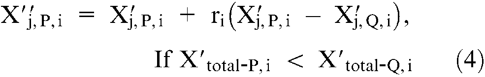
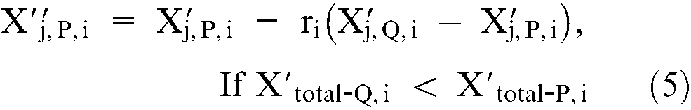
accept X″_j,P,i if it gives a better function value. All the accepted function values at the end of learner phase are maintained and these values become input to the teacher phase of the next iteration. The values of r_i used in equations (1), (4) and (5) can be different. Repeat the procedure of the teacher phase and learner phase until the termination criterion is met.

The TLBO algorithm is a parameter-free algorithm. It only requires the population size at the start. However, the population size is not considered as a parameter of this algorithm as the other algorithms like genetic algorithm (GA), artificial bee colony (ABC) algorithm, particle swarm optimization (PSO) algorithm, etc., also require a population size at the start, in addition to their respective algorithm parameters.

The next section presents the applications of this proposed algorithm for parameter optimization of the LBW process.

Application examples

Example 1

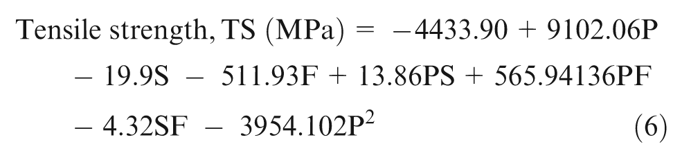
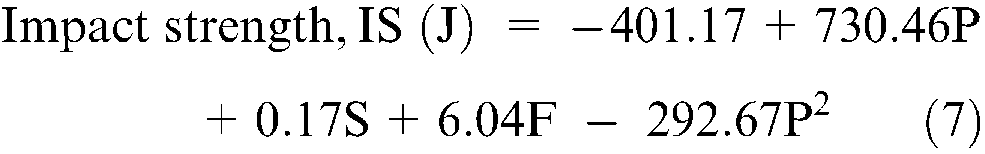
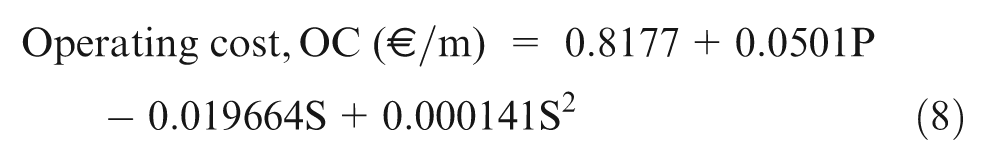
The multi-objective LBW process model attempted by Benyounis et al. ⁹ is considered in this example. The three conflicting objectives considered in the research work are maximization of tensile strength, maximization of impact strength and minimization of operating cost. The decision parameters involved in the model are; laser power (kW), welding speed (cm/min) and focal point position (mm). The objective functions as described by Benyounis et al. ⁹ are given by equations (6)–(8), respectively.

$$\text{Tensile strength},\text{TS}\left(\text{MPa}\right)=-4433.90+9102.06\text{P}-19.9\text{S}-511.93\text{F}+13.86\text{PS}+565.94136\text{PF}-4.32\text{SF}-3954.102{\text{P}}^2$$

(6)

$$\text{Impact strength},\text{IS}\left(\text{J}\right)=-401.17+730.46\text{P}+0.17\text{S}+6.04\text{F}-292.67{\text{P}}^2$$

(7)

$$\text{Operating cost},\text{OC}(€/\text{m})=0.8177+0.0501\text{P}-0.019664\text{S}+0.000141{\text{S}}^2$$

(8)

The lower and upper bounds for laser power, welding speed and focus position are given by equations (9)–(11), respectively.

$$\text{Laser power}\left(\text{P}\right)=1.03-1.37\text{kW}$$

(9)

$$\text{Welding speed}\left(\text{S}\right)=26.48-68.52\text{cm}/\text{min}$$

(10)

$$\text{Focus position}\left(\text{F}\right)=-1-0\text{mm}$$

(11)

Benyounis et al. ⁹ designed experimental tests using a three-factor five-level central composite rotatable design with full replication. Statistical software Design-Expert V7 was used and the response surface methodology (RSM) models were obtained for each response. The desirability method was used to solve optimization problems.

The output of the work obtained by Benyounis et al. ⁹ gives a pareto optimal set of solutions to obtain maximum tensile strength of 670 MPa, maximum impact strength of about 39 J and the minimum operating cost of about 0.2052 €/m. However, to check for further improvement in these results, the same model is now attempted using the proposed TLBO algorithm.

The proposed TLBO algorithm is applied to this multi-objective optimization model with a population size of 10 and the results are obtained in very few generations. The individual convergence results are shown in Figures 1–3. The combined objective function was not reported by Benyounis et al. ⁹ ; however, the same is calculated and presented in the present work. The results obtained for individual objective functions are explained below:

Figure 1.

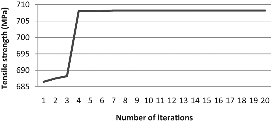
Convergence of result for tensile strength.

Figure 2.

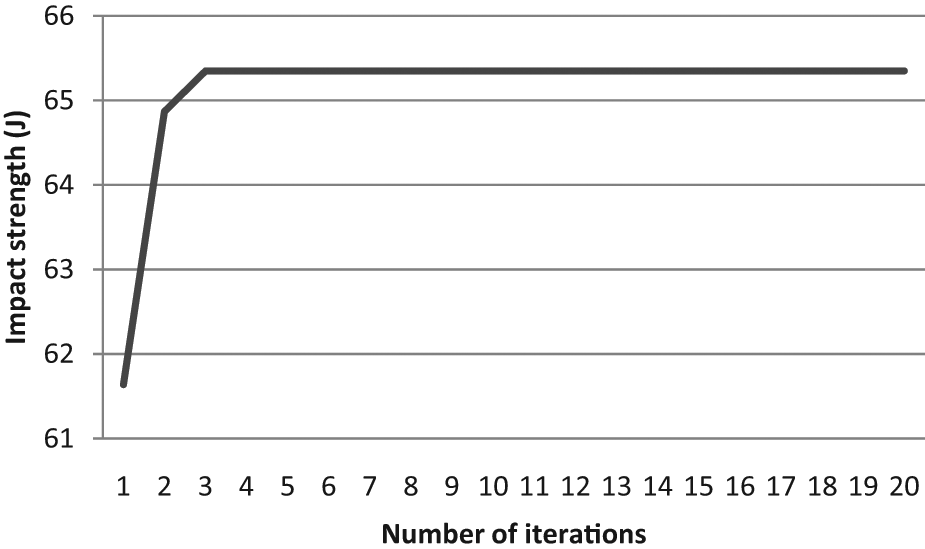
Convergence of result for impact strength.

Figure 3.

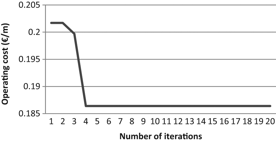
Convergence of result for operating cost.

Optimization of single objective functions

The mathematical model for the tensile strength is given by equation (6). Benyounis et al. ⁹ reported a maximum tensile strength of 670 MPa using statistical Design Expert V7 software. For this maximum tensile strength, the suggested parameter setting by Benyounis et al. ⁹ and the parameter setting obtained by the proposed TLBO algorithm are given in Table 1. It has been observed that the proposed TLBO algorithm has consistently reported a tensile strength of above 708 MPa, which is 5% more than that reported by Benyounis et al. ⁹ The convergence of results is shown in Figure 1.

Table 1.

Optimum results obtained for single objective functions of example 1

Parameters	Results of Benyounis et al. 9			TLBO Results
	TS (MPa)	IS (J)	OC (€/m)	TS (MPa)	IS (J)	OC (€/m)
Laser power (kW)	1.22	1.22	1.22	1.1974	1.2629	1.0318
Welding speed (cm/min)	60	60	60	26.48	63.5504	65.4520
Focused position (mm)	-0.8	-0.8	-0.8	0	0	0
Objective function value	670	39	0.2051	708	65	0.1864

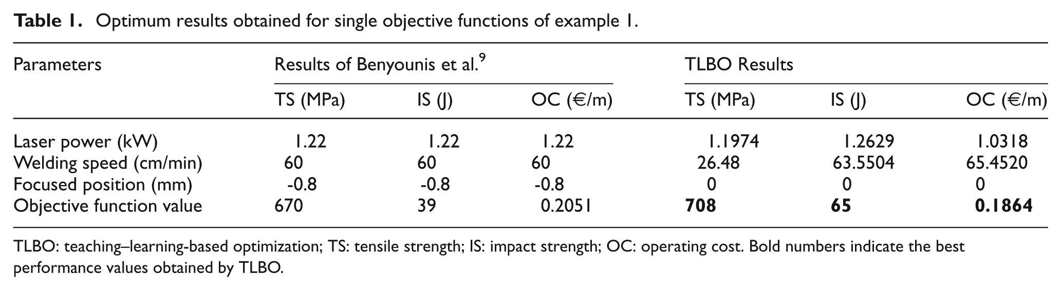
TLBO: teaching–learning-based optimization; TS: tensile strength; IS: impact strength; OC: operating cost. Bold numbers indicate the best performance values obtained by TLBO.

Equation (7) shows a mathematical model of impact strength. Benyounis et al. ⁹ reported the maximum impact strength of 39 J whereas, application of the proposed TLBO algorithm has given a much better impact strength of above 65 J. The optimum design parameters for impact strength obtained by Benyounis et al. ⁹ and the TLBO algorithm are given in Table 1 and the convergence of TLBO result is shown in Figure 2. The TLBO algorithm has reported the improvement in impact strength of above 66% over that obtained by Benyounis et al. ⁹ The convergence of results was also very fast and the result was obtained in third iteration only. Such significant improvement in the result indicates the superiority of the proposed algorithm towards the global optimum solution.

The operating cost function given by equation (8) clearly shows that the cost depends only on laser power and welding speed, whereas variation in focus position does not affect the operating cost. The minimum operating cost reported by Benyounis et al. ⁹ was 0.2051 €/m for which the optimized parameters are given in Table 1. Application of the TLBO algorithm to the same model of operating cost has reduced the operating cost to 0.1864 €/m, which is comparatively lower than the result reported by Benyounis et al. ⁹ The optimum design parameters for this operating cost obtained by the TLBO algorithm are given in Table 1 whereas the convergence of result is shown in Figure 3. The TLBO algorithm has reported over 9% improvement in the operating cost as compared to the result reported by Benyounis et al. ⁹

Optimization of combined objective function

In the present research, an attempt is carried out to obtain parameter setting in such a way that all the conflicting objectives are satisfied simultaneously. For this purpose, a combined objective function is obtained by normalizing all the individual objectives and assigning some weightages to each of these objectives. ¹⁵ The combined objective function obtained for the present work is given by equation (12)

$$\text{Min Z}=-{\text{W}}_1*(\text{TS}/\text{T}{\text{S}}_{\text{max}})-{\text{W}}_2*(\text{IS}/\text{I}{\text{S}}_{\text{max}})+{\text{W}}_3*(\text{OC}/\text{O}{\text{C}}_{\text{min}})$$

(12)

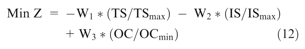
where, W₁, W₂ and W₃ are the weightages assigned to individual models of tensile strength (TS), impact strength (IS) and operating cost (OC), respectively. In the present case, equal weightage of 1/3 is given to all the respective models. TS_max and IS_max are the maximum responses reported by the respective models when these objectives are attempted separately. Similarly, OC_min is the minimum value reported by the operating cost model. The TLBO algorithm is applied to this combined objective function and the optimum parameters setting and the optimum results obtained by the algorithm are given in Table 2.

Table 2.

Optimum results obtained for the combined objective function of example 1.

Parameters	Optimum result
Laser power (kW)	1.2084
Welding speed (cm/min)	67.3472
Focused position (mm)	−1.0
Tensile strength (MPa)	697.8664
Impact strength (J)	59.5609
Operating cost (€/m)	0.1935

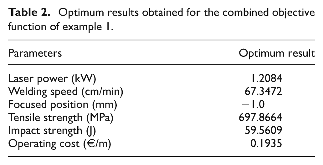
The optimum result obtained by using the combined objective function also gives the result near to the individual function value. If any particular objective is very critical in decision making, then the respective weightage may be varied accordingly to obtain the optimum parameter setting.

Example 2

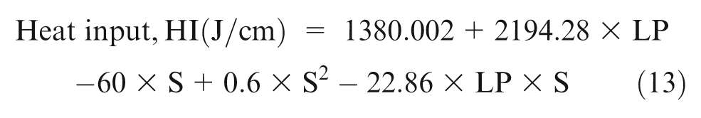
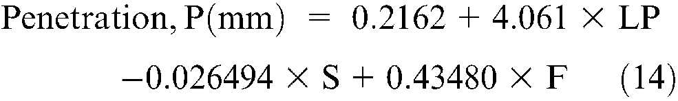
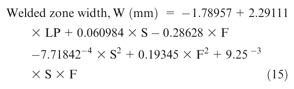
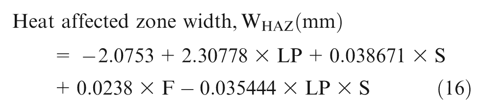
Another example is taken from the work of Benyounis et al. ³ In this work, Benyounis et al. ³ considered four different conflicting objectives related to heat input (J/cm), penetration (mm), welded zone width (mm) and heat affected zone width (mm). Various input parameters involved in the mathematical models are laser power (kW), welding speed (cm/min) and focus position (mm). The mathematical models, as given by Benyounis et al., ³ are given by equations (13)–(16).

$$\text{Heat input},\text{HI}(\text{J}/\text{cm})=1380.002+2194.28\times \text{LP}-60\times \text{S}+0.6\times {\text{S}}^2-22.86\times \text{LP}\times \text{S}$$

(13)

$$\text{Penetration},\text{P}\left(\text{mm}\right)=0.2162+4.061\times \text{LP}-0.026494\times \text{S}+0.43480\times \text{F}$$

(14)

$$\text{Welded zone width},\text{W}\left(\text{mm}\right)=-1.78957+2.29111\times \text{LP}+0.060984\times \text{S}-0.28628\times \text{F}-7.71842^{-4}\times {\text{S}}^2+0.19345\times {\text{F}}^2+9.25^{-3}\times \text{S}\times \text{F}$$

(15)

$$\begin{array}{c}\multicolumn{1}{c}{\text{Heat affected zone width},{\text{W}}_{\text{HAZ}}\left(\text{mm}\right)=-2.0753+2.30778\times \text{LP}+0.038671\times \text{S}+0.0238\times \text{F}-0.035444\times \text{LP}\times \text{S}}\end{array}$$

(16)

The lower and upper bounds for the input parameters involved in the models are given by equations (17)–(19)

$$\text{Laser power}\left(\text{LP}\right)=1.2-1.425\text{kW}$$

(17)

$$\text{Welding speed}\left(\text{S}\right)=30-70\text{cm}/\text{min}$$

(18)

$$\text{Focus position}\left(\text{F}\right)=-2.5-0\text{mm}$$

(19)

Response surface methodology was applied by Benyounis et al. ³ to the experimental data and Design-expert V6 statistical software was used to obtain linear and quadratic polynomial equations. Experimentation was conducted on the 5 mm thick plate of medium carbon steel and the responses of heat input and weld bead geometry were predicted by using these equations.

The maximum heat input and penetration reported by Benyounis et al. ³ were 2100 J/cm and 4.407 mm, respectively, by suggesting the input parameters of laser power = 1.31 kW, welding speed = 30 cm/min and focused position = –1.25 mm. Similarly, the minimum width of welded zone and heat affected zone reported were 2.398 mm and 0.573 mm, respectively. However, to check for the possibility of further improvement in this solution obtained by Benyounis et al., ³ the proposed TLBO algorithm is now applied to the same model. The results obtained by the algorithm for each response are discussed below.

Optimization of single objective functions

Four different objectives were reported by Benyounis et al., ³ which included heat input and various weld-bead geometries. The heat input largely depends on laser power and the welding speed. The mathematical model of heat input used by Benyounis et al. ³ is given by equation (13). Now the proposed TLBO algorithm is applied to the same model by using the population size and number of iterations as 20 each. The TLBO algorithm has given the maximum heat input of 2268 J/cm as compared with the result of 2100 J/cm reported by Benyounis et al. ³ The convergence of result is shown in Figure 4. The optimized parameter setting given by the TLBO algorithm and that reported by Benyounis et al. ³ are given in Table 3.

Figure 4.

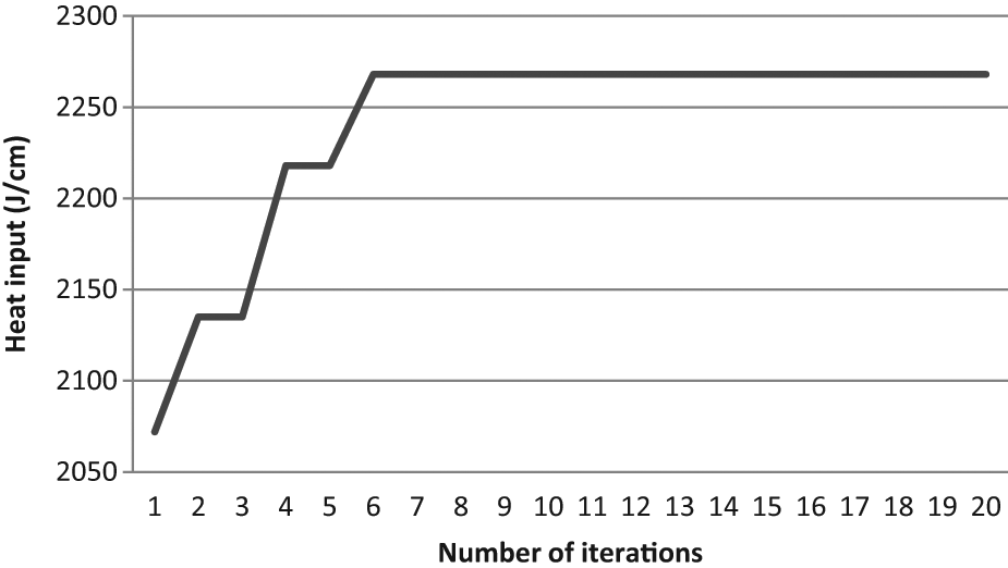
Convergence of result for heat input.

Table 3.

Optimum results obtained for single objective functions of example 2

Parameters	Results obtained by Benyounis et al. 3				TLBO Results
	HI (J/cm)	P (mm)	W (mm)	WHAZ (mm)	HI (J/cm)	P (mm)	W (mm)	WHAZ (mm)
Laser power (kW)	1.31	1.31	1.31	1.35	1.4240	1.4129	1.2011	1.4098
Welding speed (cm/min)	30	30	50	50	30	30	69.4706	69.7736
Focused position (mm)	−1.25	−1.25	0	−1.25	−0.6820	−0.1472	−0.9270	−2.3295
Objective function value	2100	4.407	2.398	0.573	2268	5.0952	1.3097	0.3345

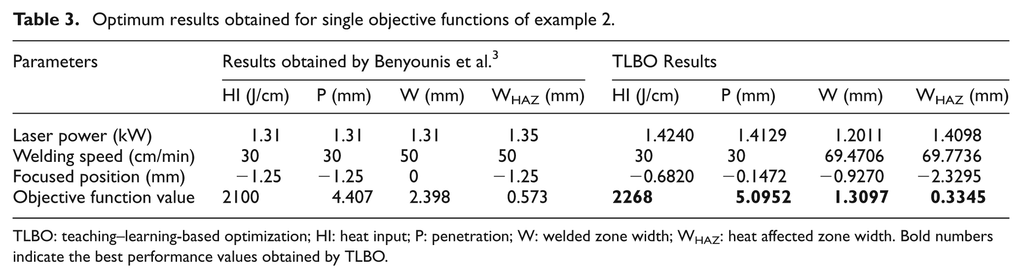
TLBO: teaching–learning-based optimization; HI: heat input; P: penetration; W: welded zone width; W_HAZ: heat affected zone width. Bold numbers indicate the best performance values obtained by TLBO

Equation (14) gives the mathematical model of penetration for which Benyounis et al. ³ showed maximum penetration of 4.407 mm. The TLBO algorithm is applied to the same model of penetration and the algorithm has given a maximum penetration of 5.0952 mm. Thus, improvement of over 15% in penetration is given by the TLBO algorithm over the result reported by Benyounis et al. ³ Figure 5 shows convergence of results by the TLBO algorithm for penetration.

Figure 5.

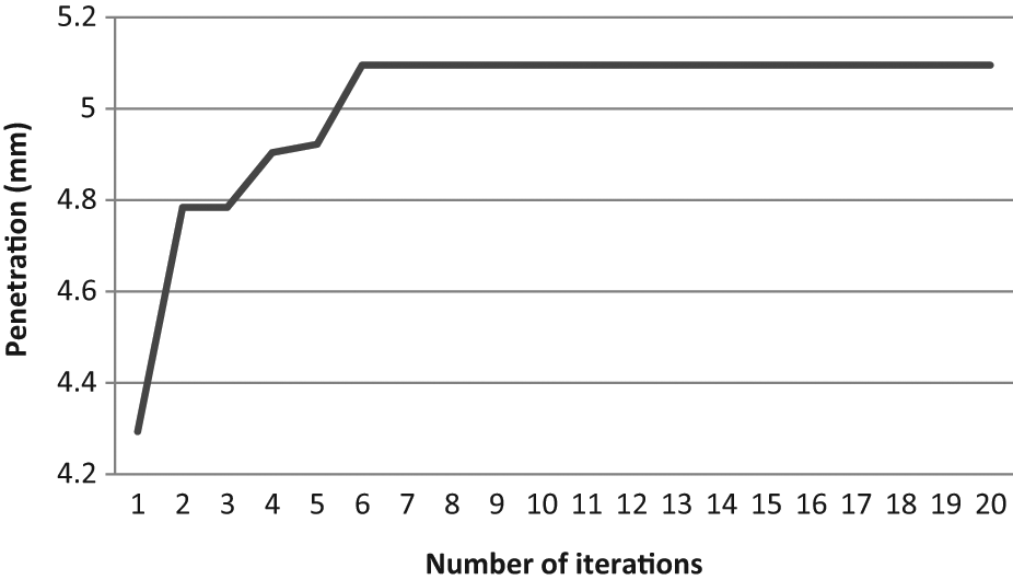
Convergence of result for penetration.

The mathematical model for welded zone width is given by equation (15). The important factors affecting the welded zone width are welding speed and focused position. Benyounis et al. ³ obtained the minimum width of the welded zone as 2.398 mm. The proposed TLBO algorithm is applied to the mathematical model of welded zone width with a population size of 20 and number of iterations of 20. The TLBO algorithm has given the minimum welded zone width of 1.3097 mm. The parameter setting obtained by the TLBO algorithm for the optimum result of the welded zone width is given in Table 3 along with the parameter settings reported by Benyounis et al. ³ In this case, the algorithm has given a significant improvement of above 45% over the result shown by Benyounis et al. ³ The convergence of result for the welded zone width is shown in Figure 6.

Figure 6.

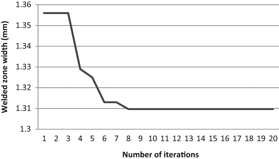
Convergence of result for welded zone width.

In the case of the heat affected zone width, Benyounis et al. ³ showed the welding speed as an influencing factor. The mathematical model for the heat affected zone width is given by the equation (16). The minimum heat affected zone width reported by Benyounis et al. ³ was 0.573 mm. The proposed TLBO algorithm is applied to the mathematical model of heat affected zone width with a population size and number of iterations of 20 each. The minimum heat affected zone width obtained by using the TLBO algorithm is 0.3345 mm. The parameter setting for this optimum result obtained by the TLBO algorithm and the parameter setting suggested by Benyounis et al. ³ for the minimum heat affected zone width are given in Table 3 and convergence of result is shown in Figure 7. The result of this model is also improved by over 34% using the TLBO algorithm.

Figure 7.

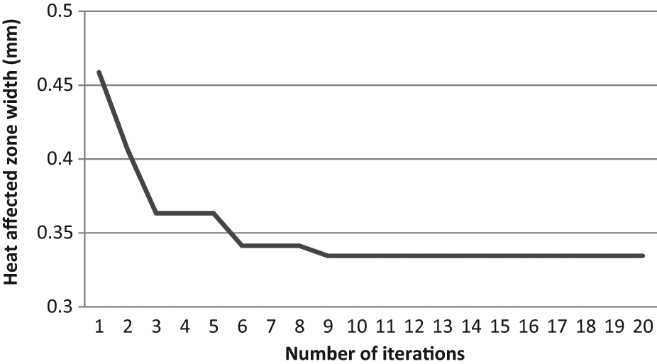
Convergence of result for heat affected zone width.

Optimization of combined objective function

In the work of Benyounis et al., ³ all four objectives were handled individually and separate optimum parameters were obtained for each objective. However, in the present work, the multi-objective problem is attempted by combining all four objectives and assigning weightages to each objective. This will give common optimum parameters that will satisfy all the objectives and constraints and also it will prove the effectiveness of the proposed algorithm. The combined objective function for the four individual responses represented by equations (13) to (17) is given by equation (20)

$$\text{Min Z}=-{\text{W}}_1*(\text{HI}/\text{H}{\text{I}}_{\text{max}})-{\text{W}}_2*(\text{P}/{\text{P}}_{\text{max}})+{\text{W}}_3*(\text{W}/{\text{W}}_{\text{min}})+{\text{W}}_4*({\text{W}}_{\text{HAZ}}/{\text{W}}_{\text{HAZ}(\text{min})})$$

(20)

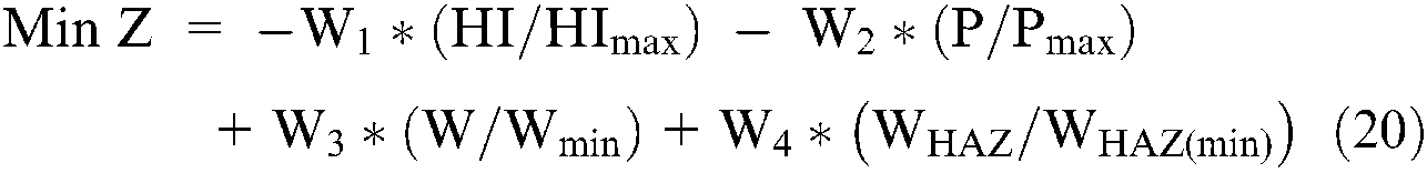
where, W₁, W₂, W₃ and W₄ are the weightages assigned to individual model of heat input (HI), penetration (P), welded zone width (W) and heat affected zone width (W_HAZ), respectively. In the present case, equal weightage of 0.25 is given to all the respective models. HI_max and P_max are the maximum response reported by the respective model when it is attempted separately. Similarly, W_min and W_HAZ(min) are the individual minimum values reported by respective models. The minimum combined objective function value reported by the TLBO algorithm for the present case is 0.4085 and the optimum parameter setting and optimum results obtained by the algorithm are given in Table 4.

Table 4.

Optimum results obtained for combined objective function of example 2.

Parameters	Optimum result
Laser power (kW)	1.20
Welding speed (cm/min)	30
Focused position (mm)	0
Heat input (J/cm)	1930.2
Penetration (mm)	4.2946
Welded zone width (mm)	2.0946
Heat affected zone width (mm)	0.5782

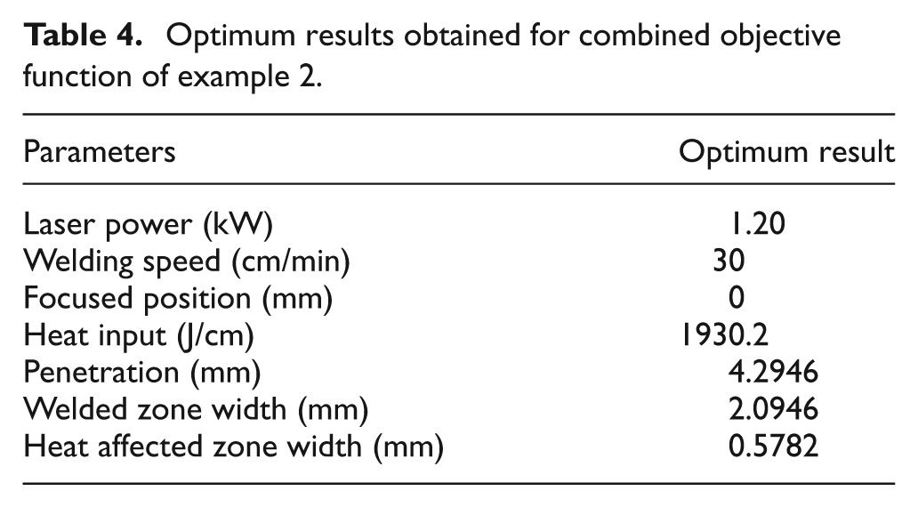
The combined objective function always gives a compromising result by satisfying all the objectives. In the present case the optimized parameters setting, also obtained by using the TLBO algorithm, has given the compromising solution for the combined objective function. The results obtained by the TLBO algorithm have proved its capability in terms of handling the multi-objective optimization problems.

Conclusion

The research work reported in this article is focused on the multi-objective multi-parameter optimization of industrial LBW process using a recently developed TLBO algorithm. Unlike other advanced optimization algorithms, this algorithm is parameter free. Two different examples are considered that consist of multi-objective models. The TLBO algorithm has given significant improvement in the results compared with the results reported by Benyounis et al.^3,9 In the first example, the optimized process parameters given by the TLBO algorithm have increased the tensile strength from 670 MPa to 708 MPa, impact strength from 39 J to 65 J and have decreased the operating cost from 0.2051 €/m to 0.1864 €/m. Similarly, in the second example, the optimized process parameters given by the TLBO algorithm have increased the heat input from 2100 J/cm to 2268 J/cm, penetration from 4.407 mm to 5.0952 mm and have reduced the welded zone width from 2.398 mm to 1.3097 mm, and heat affected zone width from 0.573 mm to 0.3345 mm.

The proposed TLBO algorithm has proved its superiority in terms of better results and faster rate of convergence for multi-objective models, as well as the individual objective functions considered in the present work. Such kind of improvement will definitely help industries to increase weld quality and to minimize production cost. This new method can also be used for parameter optimization of other manufacturing processes.