
Abstract
Drying of ceramic parts with complex geometry has been studied with emphasis on the effects of shrinkage on their final dimensions. The first step was to understand the processes governing moisture loss from a porous medium through experimental measurements yielding the coefficient of moisture expansion. As a result, non-homogeneous dimensional changes (shrinkage) occur in three-dimensional artefacts with varying cross-section. The moisture diffusion problem governed by Fick’s laws was solved numerically by analogy to the heat conduction problem. To this end the correspondence was established between physical parameters, variables and boundary conditions of heat flow and diffusion, characteristically the coefficient of moisture expansion being analogous to the coefficient of thermal expansion. The numerical model established and solved using finite element analysis predicted moisture distribution inside the part as well as the resulting change in its shape. Validation of numerical predictions was first ensured in two dimensions by modelling a simple slab and comparing with experimental measurements. Validation for a fully three-dimensional shape required use of the well-established iterative closest point algorithm for surface point matching and subsequently the creation of an error map. The reverse of this numerical model was used to predict the appropriate die geometry starting with the shape of the desired part by taking into account the variable drying shrinkage allowance, and the relevant steps are outlined.
Keywords
Introduction
Many manufacturing processes employ closed cavity dies or moulds. The material being processed is fed into the die or mould either in liquid phase or in semi-solid/semi-liquid phase and, while undergoing solidification, it also shrinks to some extent depending on the nature of the process and of the material itself. It is important for the designer of the die or mould to account for the shrinkage in order to achieve accuracy of shape and dimensions of the final part. This task becomes a challenge even when medium accuracy is required in view of the different amounts of shrinkage that each area of the part may exhibit. This is conspicuous when part shape is not regular and consists of consecutive sections whose area varies intensely, which is typical in sculptured surfaces.
In the particular case of ceramic part manufacturing using dies and moulds, the need for exact calculation of shrinkage can be addressed by modelling the drying process governed by Fick’s laws1,2 using finite element analysis (FEA).3,4
Diffusion coefficient depends on temperature, moisture content 2 and even on shrinkage 3 but it is usually taken as a constant – mean – value representative of the particular application. However, since diffusion coefficient is determined experimentally, an accurate investigation of its individual dependency on particular factors is not necessary, certainly not in the scope of this work. Besides diffusion other mass transfer mechanisms such as a combination of capillary and surface diffusion, Knudsen, Stefan and mutual diffusion or even Pouiseuille flow are either not applicable or have a negligible influence in free drying of clay. 3 Nevertheless, any potential presence of such mechanisms will automatically be embedded in the experimental measurement of diffusion coefficient in the context of Fick’s law. The latter may be replaced by Darcy’s law to model cases where mean velocity of the liquid phase depends on the flow potential that is generated by pressure differential through porous media and by the influence of gravity. 5 However, for isothermal drying in a liquid–solid system, pressure differential corresponds to moisture concentration differential, i.e. Darcy’s law is replaced by Fick’s law. Isothermal drying is taking place when energy input into the drying system balances the energy used for moisture vaporization, in the case of forced drying, or moisture evaporation, in the case of free drying in ambient temperature. This allows the temperature field to be neglected in the equations describing moisture distribution. 6
Shrinkage prediction has been addressed in drying system simulation literature only in the last few years. 7 The problem is one of moving boundary, being tackled in different ways. The simplest and commonest approach is to consider that shrinkage is due exclusively to moisture removal and derive equations relating geometric dimensions with moisture concentration. These equations are semi-empirical and can be applied to relatively simple shapes. They are used to generate the moving boundary on which the drying model is applied. Concerning mesh movement, it is possible to either re-determine stepwise the solution space at each time step or to employ the local deformation velocity of the material. One approach considers mesh movements according to experimentally determined stress–strain relationships. 8 Another approach involves superposition of Lagrangian and Euclidean reference systems 9 under the assumption that the shrinkage percentage is proportional to moisture removal; however, it is difficult to determine the effect of porosity on this assumption. 10 Thermal expansion needs also to be accounted for in non-isothermal drying. In addition, mechanical resistance – internal friction – mechanisms might become important, too. In view of the complexity of the mechanisms connected to shrinkage in drying systems and the lack of a universally adopted theoretical background, the approach adopted in the present work is analogous to that employed in thermal barrier calculations in space vehicles 11 and space telescopes, 12 i.e. experimental determination of the coefficient of moisture expansion (CME).
Numerical methods used in the literature assume that for adequately small time steps transfer conditions and part dimensions remain practically constant. Therefore, shrinkage is neglected in computing moisture content for the next time step. Then, shape is computed anew as well as the transfer conditions. The process is repeated until drying is completed.
Even after accurate prediction of the shape and dimensions of the part after shrinkage, the attained accuracy has to be derived by comparing to the ideal shape and dimensions. This requires optimum relative positioning of the ideal and the real parts as well as a robust and adequately descriptive method for quantifying their similarity. 13 Proper alignment of the two surfaces is achieved by the widely used iterative closest point (ICP) algorithm.14,15 The generation of colour-coded maps is widely used to evaluate the form error of sculptured surfaces. 16 These error maps contain information for the dimensional deviation of a manufactured free-form surface from the one designed in the computer-aided design (CAD) program, mapped onto the part geometry. In our case this method is used to compare the model predicted surface with the one measured in the laboratory.
Prediction of a suitably deformed cavity in the case of ceramic part manufacturing using dies and moulds is the third issue tackled in this paper. Further to predicting the final part shape and comparing it to the ideal, the ultimate goal is to design the die or mould that would produce the part as close to the ideal as possible. Naturally, a large amount of research has been carried out concerning proper tooling design that minimizes process-related defects of final parts which can be attributed to excessive local shrinkage, usually coupled with the rheological behaviour of the processed material. We are instead focusing on addressing global shrinkage and its effects on dimensional accuracy of the final product. In this regard any die or mould, even when designed to avoid the aforementioned effects, by default produces parts that differ geometrically from the ideal. There has been some research concerning prediction of shrinkage for the net-shape processes of injection-moulded parts17,18 and investment cast parts. 19 Especially in the latter case, two steps of shrinkage prediction should be performed, one for the wax patterns and one for the actual part. A few research teams have actually incorporated a ‘reverse deformation method’ in die and mould design, either by considering shrinkage factors 20 or FEA. 21
Shrinkage and moisture measurements concerning the drying of cast and pressed clay parts are presented first. Numerical models for shrinkage prediction are outlined next and the corresponding results obtained using a commercially available FEA package are presented. The methods used to compare ideal and shrunk part models are explained next with implementation details and results. The issue of computing the appropriate die shape to yield the required part shape is presented last, followed by a discussion and conclusions.
Experimental
Initial investigation
Moisture content and shrinkage were measured as a function of drying time for two different parts. The first was a stepped slab consisting of three consecutive progressively smaller parallelepipeds, see Figure 1, made of hard fayence, manufactured by pressing clay into a die. The second part was a sculptured face, see Figure 2, made of soft fayence, manufactured by casting clay into a die and making it, by contrast to the stepped slab, a shell with wall thickness of approximately 7 mm.
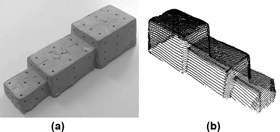
Stepped slab: (a) clay prototype; (b) scanning line model.

Sculptured face: (a) clay prototype; (b) scanned surface model.
Moisture evaporation was measured by weighing the parts every 24 h using precision scales, see Figure 3. Drying was considered to be complete when moisture evaporation in 24 h was less than 1/1000 of the original part weight.
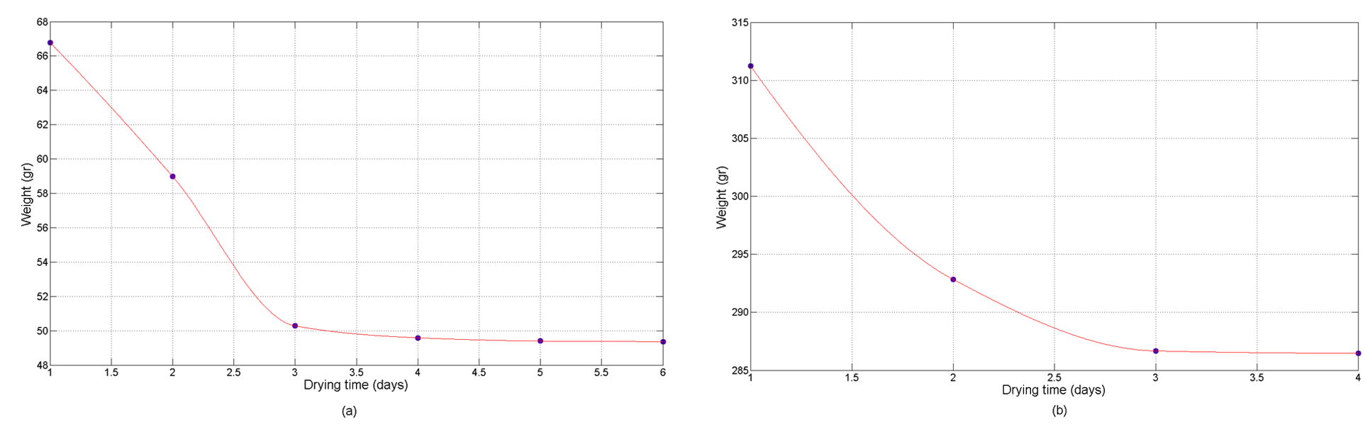
Weight variation in the drying process: (a) stepped slab; (b) sculptured face.
Shrinkage was determined by first scanning the parts and building digital models, which then enabled accurate measurements of linear distances between specific reference points on the part surface taken on a CAD system. These points had been engraved on the parts as soon as these were ejected from the respective dies, see Figures 1(a) and 2(a). The stepped slab was simple enough to scan in less than 30 min using a Hawk 222 laser scanner equipped with a Renishaw Wizprobe head. Reasonable scanning time was crucial, to ensure that no noticeable shrinkage occurred in a complete scanning session. For this reason, the face part, which was much more complex in shape, was scanned on a GOM ATOS I white light scanner on which the complete scanning session took just a few minutes. The three-dimensional (3D) models were constructed from the scanned point clouds using proprietary software of the two scanning systems at an intermediate level to construct a surface triangular mesh in STL representation, followed by surface fitting and transformation into solid using the Rhinoceros CAD software.
Shrinkage of the two parts is shown in Figure 4 across sections based on scanned point clouds. The prismatic part exhibits uniform shrinkage in the horizontal and in the vertical direction on all sections normal to its longitudinal plane. Shrinkage seems more pronounced in the vertical direction. The sculptured part exhibits non-uniform shrinkage at both lateral and longitudinal cross-sections.

Shrinkage between initial (outer profiles) and final scanned (inner profiles) forms: (a) stepped slab – lateral cross-section; (b) sculptured face – lateral cross-section; (c) sculptured face – longitudinal cross-section.
Figure 5(a) presents shrinkage of the stepped slab with time across the width of the three parallelepipeds. The three parallelepipeds shrink by different ratios, i.e. 5.76%, 4.78% and 3.90% from the largest to the smallest, respectively. The polygonal lines joining the three series of reference points along the longitudinal axis of the part, see Figure 1(a), show no significant difference in shrinkage, its mean final value being 4.15%. Figure 5(b) presents shrinkage of the four lines that join reference points of the sculptured face part along two directions as shown in Figure 2(a), ranging between 7.05% and 7.9%. There is no obvious correlation in this case, since each line crosses through continuously varying sections of the part.
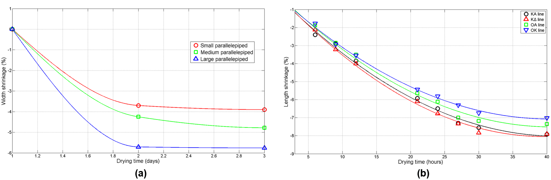
Linear shrinkage of reference lines: (a) stepped slab width; (b) sculptured face.
Coefficient of moisture expansion
In any theoretical model of clay drying it is important to express shrinkage as a function of moisture loss. In this work the correspondence between moisture systems and thermal systems is advanced further by considering shrinkage due to moisture loss by analogy to contraction due to heat loss, based on reports from space programmes on ceramic and polymer materials.11,12 A CME is defined, by analogy to the coefficient of thermal expansion (CTE), as

where ΔL is the difference in reference length Lref, β is the CME, Mf is moisture content in the final state and Mref is moisture content in the reference state. Moisture content is calculated as
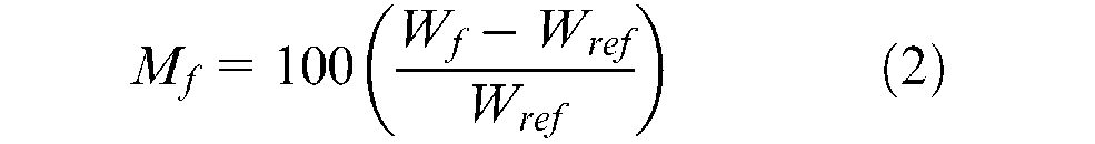
where Wf and Wref are specimen mass in the final and the reference state, respectively.
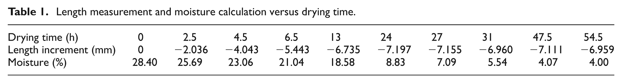
CME was calculated on a specimen made from the material under investigation in the form of a long slab, using a die of 145 mm × 20 mm × 25 mm. In the case of soft fayence initial moisture content was 28%. This was left to dry naturally in the atmosphere (4% moisture at the time of the experiment), and its weight and length were measured regularly. Application of equation (2) gives the results shown in Table 1. Then, application of equation (1) gives the value of CME as 20.29 × 10⁻³.
Length measurement and moisture calculation versus drying time.
Numerical modelling of clay drying
Diffusion analogy to heat conduction
Fick’s law of diffusion has an obvious analogy to Fourier’s law of heat conduction – hence the term ‘diffusion analogy’. 22 The theory of diffusion in isotropic media is based on the hypothesis that the rate of mass transfer of diffusing substance through unit area of a section is proportional to the concentration gradient measured normal to the section. It is expressed mathematically by the following equation

where F is the rate of transfer per unit area of the section, C is the concentration of diffusing substance, x is the spatial coordinate measured normal to the section and D is the diffusion coefficient. Equation (3) represents Fick’s First Law for one-dimensional systems. The minus sign denotes that diffusion occurs in a direction that is opposite to the increase in concentration.
Fick’s First Law is complemented by the following equation, which applies to time-dependent one-dimensional systems, and constitutes Fick’s Second Law

Equations (3) and (4) can easily be modified to accommodate two-dimensional (2D) and 3D systems, as well as anisotropic media.
In order to benefit from the wealth of solutions of the heat conduction equations, the correspondence between physical parameters, variables and boundary conditions of heat flow and diffusion problems should be examined. The relevant heat flow equations are presented below


where θ is temperature, K is heat conductivity, ρ is density and c is specific heat, so that cρ is heat capacity per unit volume, x and t are space and time coordinates, and F is the amount of heat flowing in the direction of x, increasing per unit time through unit area of a section which is normal to the direction of x.
In order that the two sets of equations, equations (3) and (5) and equations (4) and (6), should correspond, one may identify concentration C with temperature θ and take
Regarding correspondence between boundary conditions, the most important in the case of free drying of clay is: prescribed surface temperature corresponds to prescribed concentration just within the surface. This is the only boundary condition relevant to this study; a comprehensive list can be found elsewhere. 22
To summarize, by solving equations (3) and (4) we determine the evolution of moisture distribution inside the part and its shrinkage due to moisture evaporation is determined through equation (1).
Slab drying pilot model (2D)
In order to build a model that predicts shrinkage caused by drying of a clay part, it is necessary to determine two coefficients: the diffusion coefficient D and the CME. While the former is commonly used and can be found in the literature, the latter has been calculated experimentally, see subsection ‘Coefficient of moisture expansion’, and needs to be verified through a corresponding model. Thus, a simple 2D pilot model of a slab drying is built, which duplicates the experimental configuration. If the model is able to accurately predict the slab length during and at the end of drying, then the method of using CME to model shrinkage of more complex parts should be plausible.
The pilot model is built and solved using the commercial FEA package ANSYS. The diffusion analogy discussed in subsection ‘Diffusion analogy to heat conduction’ allows the use of thermal elements to create a pseudo-thermal field where temperature corresponds to moisture and physical parameters and boundary conditions are chosen accordingly. Structural elements are also used, so the model is able to account for deformation due to shrinkage effects. The coupling between thermal and structural fields can be achieved in one of two ways.
First, a solution is obtained for the transient pseudo-thermal field. Then the calculated moisture distribution at the end of drying (the last time step of the transient analysis) is fed as input (loading) to the structural field, which, in turn, calculates the expected deformation of the part. This method ignores the intermediate effects of deformation on moisture distribution during drying (all but the last step of drying are accounted for), but is fast and computationally inexpensive.
Alternatively, special coupled-field elements are used which are able to handle thermal as well as structural loads. The solution is obtained through direct-coupled field analysis of the transient problem. At the end of each time step the pseudo-thermal solution is used to calculate the structural field deformation, which in turn is taken into consideration during the next time step. This dynamic interaction between pseudo-thermal and structural fields continues throughout all the subsequent time steps, until the drying process is complete. This method simulates the actual process more realistically and accurately, at the expense of being slower and more computationally expensive.
In order to verify the experimentally determined CME, the model should produce shrinkage data for intermediate times during the drying process, ideally corresponding to the measuring times of the experiment; thus the second method is used. The modelling philosophy and necessary steps to build the pilot model within the ANSYS environment are presented below.
A 2D eight-node solid element appropriate for modelling slabs is chosen (plane223) and designated as coupled-field element (thermal-structural, keyopt11). Next, material properties are input; diffusion coefficient takes the place of heat conductivity and CME takes the place of CTE. Appropriate values for diffusion coefficient are taken from the literature, 23 while CME is set to the experimentally calculated value. Density and specific heat are set equal to unity, ensuring the creation of a pseudo-thermal field with the desired behaviour (see ‘Diffusion analogy to heat conduction’ subsection).
Part symmetry should be used in order to reduce computational load, so only half of the slab is designed as a parallelogram of appropriate dimensions which is divided into square elements with edge of 0.5 mm, see Figure 6(a).
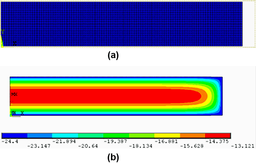
Simulation results for slab at 1 h drying time: (a) final shape; (b) moisture distribution.
For reasons relating to internal procedures within the FEA solver used, reference moisture should be set to zero, so that moisture loss leads to negative moisture values. This is purely a matter of convention and does not affect the analysis, since the equations used refer to moisture differences rather than absolute values. In addition, moisture at the free edges is set to constant −24.4%. This corresponds to free drying in atmosphere of steady moisture content, as discussed earlier. Note that for negative moisture differences, CME gives part shrinkage. Proper boundary condition for symmetry is assigned to the left edge, see Figure 6(a).
Solution options selected include enabling the small-displacement transient Newton–Raphson method, setting simulation time to 54.5 h with constant time step of 0.5 h and activation of stepped loading. Results are stored separately for all time steps.
Figure 6(a) shows slab deformation at the end of drying and Figure 6(b) shows the moisture distribution after 1 h of drying.
In order to verify the pilot model, predicted slab length is compared with experimental values at several points during the drying process. The results, which are summarized in Figure 7, exhibit good agreement between numerically predicted and experimentally measured values (0.26% relative error at complete drying). Clearly, diffusion analogy and use of CME are valid tools for predicting shrinkage due to drying of a clay part.
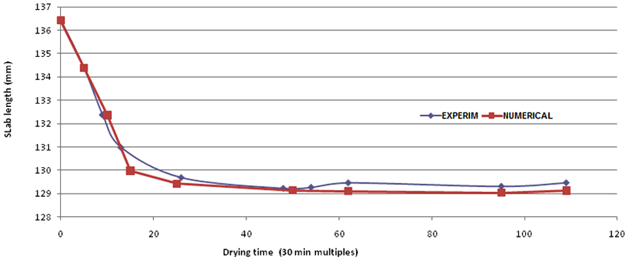
Comparison of numerically computed and experimentally measured length variation with drying time for simple slab.
Sculptured surface shrinkage drying model (3D)
The same modelling philosophy applies in the case of a free-form sculpted surface, with a few modifications required due to the more complex part geometry.
Apart from different geometry input and comparison method, a different kind of element is necessary from the one that was used in the simple 2D slab model. A 3D 10-node tetrahedral solid element is selected (solid227), which is appropriate for coupled-field modelling of complex shapes. Use of symmetry is impossible, thus the boundary condition of constant moisture is applied to the entire external surface. Material properties and solution options are set accordingly.
Figure 8(a) shows shrinkage of the part in front view, the dotted line corresponding to its initial profile. It is worth noting that its thickness deformation is negligible, which is expected since variations are more pronounced along larger dimensions. Figure 8(b) shows moisture distribution at various cross-sections after 1 h of drying.
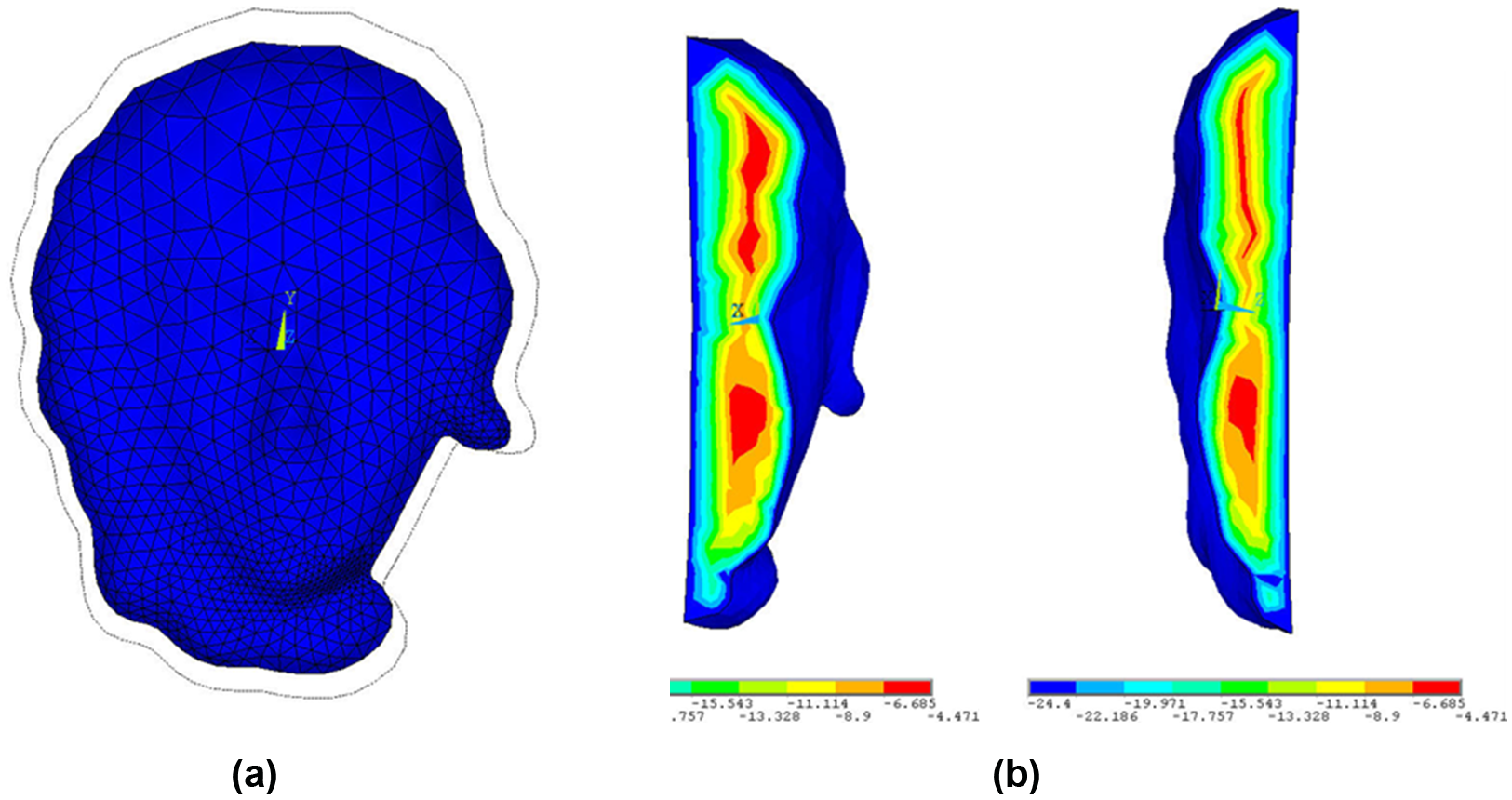
Simulation results for sculptured face at 1 h drying time: (a) final shape; (b) moisture distribution.
3D complex shape comparison for shrinkage computation
The need for quality control of free-form surfaces, used widely in many fields of modern industry, has led to advanced inspection techniques able to implement non-traditional tolerancing methods. The generation of error maps is commonly used to visualize the dimensional differences between ideal and manufactured parts. An error map is a colour-coded representation of normal deviation of each point in a cloud from the ideal surface. 16
What naturally precedes the extraction of the error map is the process of surface registration. As a general rule the coordinate system of the coordinate measuring machine used in the dimensional inspection of a complex part is different from the coordinate system of the CAD model, against which the comparison takes place. Thus the measured part and the ideal model need to be realigned. This is usually achieved through the ICP algorithm, 14 which optimally aligns two sets of points to a common coordinate system.
Surface registration through ICP algorithm
The ICP algorithm was originally proposed by Besl and McKay 14 and further developed by a number of researchers, see for instance Yu et al. 15 The idea behind it is to match each point in one cloud to its closest point in the other cloud and calculate the transformation that minimizes the root mean square distance between the two clouds.
Let QI and PJ be point clouds with I and J number of points and
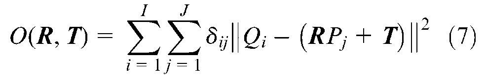
where
A simple example that illustrates the application of the ICP algorithm is presented in Figure 9. Based on the initial unaligned position of the two point sets (I), a matching of the closest points between them is generated (II). Then a transformation is calculated (III) that leads to a new matching set (IV). A final transformation leads to optimal alignment of the two clouds (V).
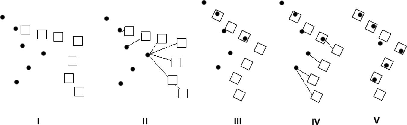
Illustration of the steps of the ICP algorithm: (I) unaligned point clouds; (II) closest point matching; (III) transformation; (IV) new matching; (V) aligned point clouds.
Error map generation
Consider the point cloud obtained from 3D scanning of the finished ceramic part. With the help of appropriate software this point cloud can be converted to a 3D surface, by smoothly interpolating or simply triangulating between its points, thus yielding a true surface representation of the actual part with precision depending on the specifics of each application. Now consider that this surface is optimally aligned with the point cloud calculated through shrinkage simulation via application of the ICP algorithm. We can visualize the local form error between actual and simulated parts by colour coding each point in the calculated cloud, based on its normal distance from the measured surface.
In the case of a triangulated surface, calculating the normal deviation is a problem of point-to-plane distance between each point in the cloud and its nearest triangle, see Figure 10. When normal shooting from multiple neighbouring triangles meet a given point, then the distance is calculated from their shared boundary to the point (P4). The same holds true if the point is met only at projections of multiple neighbouring triangles (P2).
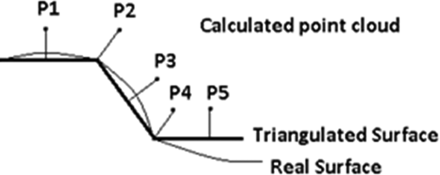
Simple representation of point-to-plane distance.
In the case of a smooth surface, calculating the normal distance of each point is more computationally expensive but yields more accurate results. Most metrology as well as some 3D modelling software packages have implemented functionality for the automatic generation of error maps, with or without triangle tessellation.
Application in 3D sculptured surface model
Two point clouds representing the shape of the sculptured face serve as input for the shape comparison computation: the cloud that results from solving the 3D shrinkage simulation (moving cloud − 19,263 points) and the one that resulted from scanning the actual part after complete drying (static cloud − 19,116 points). The static point cloud is also converted to a smooth surface with the help of the Rhinoceros software, in preparation for the extraction of the error map. Figure 11(a) shows the calculated point cloud and the smooth scanned surface before registration.
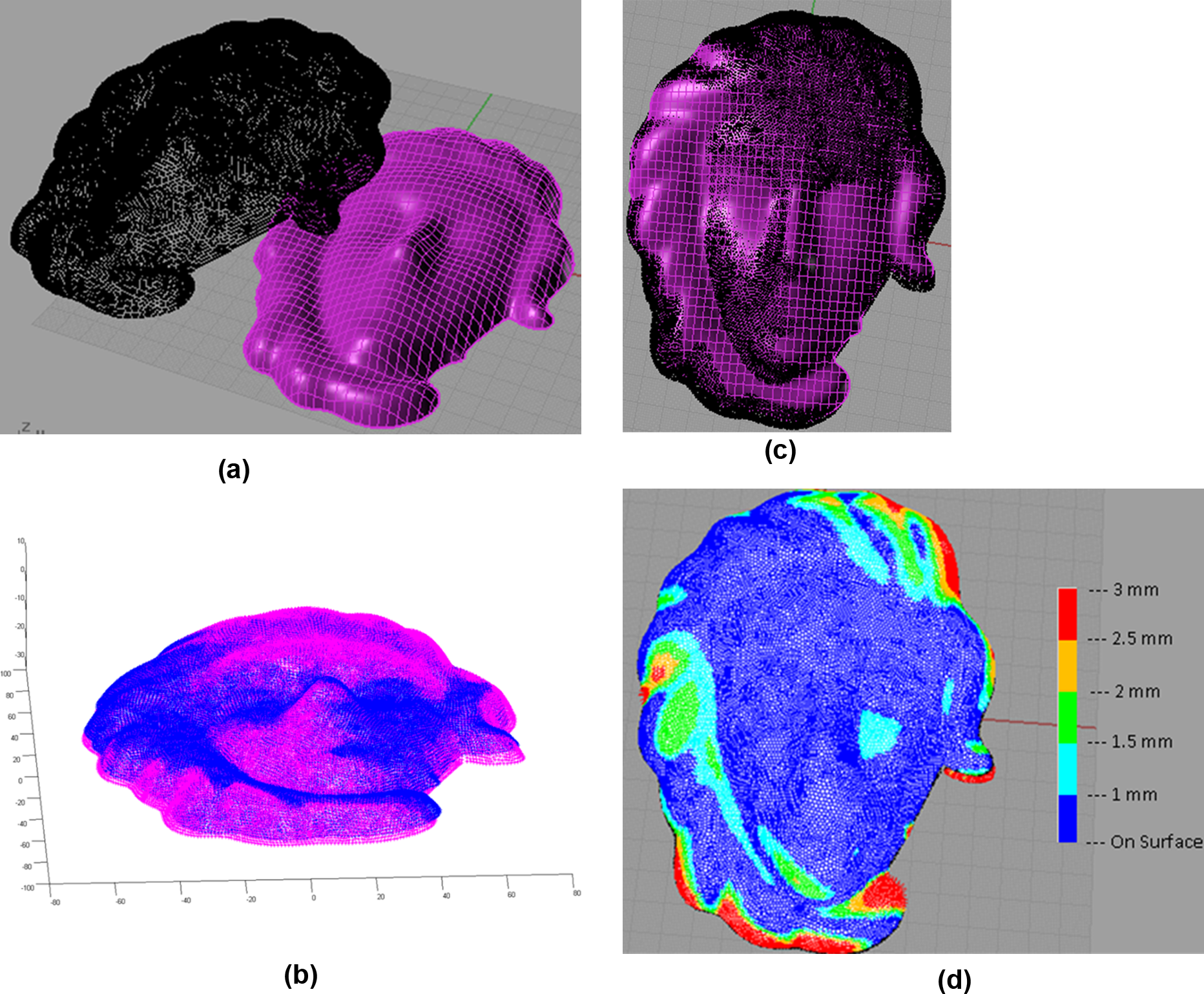
(a) Calculated point cloud and actual scanned surface in the Rhinoceros graphical environment before registration; (b) point cloud registration via ICP algorithm in MATLAB; (c) calculated point cloud and actual scanned surface in the CAD environment after registration; (d) error map of predicted point cloud in comparison to the actual scanned surface.
The two point clouds are aligned by means of the ICP algorithm implemented in MATLAB. An outline of the necessary steps is given below:
Input point clouds to be registered in matrix form.
Initialize parameters.
Optimization loop: Determine closest points. Calculate transformation. Apply transformation. Check for convergence.
Save optimal rotation and translation matrices.
Apply optimal transformation to moving point cloud.
Plot registration in 3D.
Figure 11(b) shows a 3D plot of the registered point clouds. After the optimal transformation of the moving cloud is applied, the result is re-imported into the Rhinoceros software. The resulting proper alignment of the moving cloud and the scanned surface is shown in Figure 11(c). An error map of absolute distance between the predicted point cloud and the real surface is automatically generated by the software and is shown in Figure 11(d). It can be seen that the majority of points lie close to the surface. The agreement between predicted and actual part in 3D is satisfactory; namely mean absolute distance is 799
Die modelling
Drying shrinkage allowance computation methodology
The philosophy for modelling clay part shrinkage discussed earlier is based on diffusion analogy and the use of a CME, rather than dealing directly with the intricacies of moisture transport and evaporation. This enables ‘inverting’ the model in order to calculate the required die/mould shape for producing a part of desired geometry. This ‘reverse shrinkage model’ does not correspond to some natural process, as there is no actual moisture absorption taking place. Nevertheless it is a useful tool that fulfils a very tangible need: to compute drying shrinkage allowance for die modelling.
The ‘reverse shrinkage’ model is built with the same method described in detail in the subsection ‘Sculptured surface shrinkage drying model (3D)’, with a few minor differences concerning input and loading. First, in the forward model a solid obtained by scanning of the mould served as input. In the reverse case the die shape is not given but rather the desired output of the model. Thus in this case, a 3D model of the final part is used as geometry input. Second, the loading must also be reversed. It is reminded that in the original model initial moisture content was set to zero, which is merely a convention, and the outer surface ‘loading’ received negative values, in order to simulate moisture loss and, consequently, shrinkage. All that is needed is to use the same absolute values of moisture on outer surfaces, only with a positive sign this time. This way the goal of reversing the moisture loss is realized. Simply put, by these simple modifications, an inverted history of the drying process is simulated and the original shape of the part at the time it exited the mould is calculated, which constitutes the desired die geometry.
Post-processing of reverse simulation results
Figure 12(a) shows a contour plot of predicted die shape superimposed on the final part shape (mesh), in the case of a bust of Hippocrates. The two shapes are arbitrarily aligned in the centre of the circular blue area; the plot’s usefulness is clearly inspectional for the purpose of die modelling.
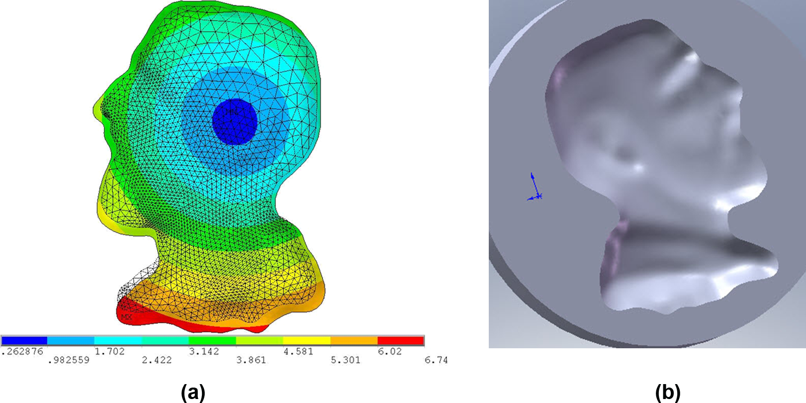
Die shape: (a) projection superimposed on final part shape; (b) negative volume in 3D.
The first step is to filter out results that are not relevant to our specific needs. The reason behind this is that solution data regarding interior nodes are only useful in the forward model, where one needs to monitor the drying process inside the part. In the reverse case of predicting the die cavity shape, only deformation data for the outer surface of the model are needed. These are obtained by selecting all the nodes lying on the exterior of the part (select > entities… nodes… from full… exterior) and saving their initial coordinates in matrix form (list > nodes… coordinates), as well as their relative displacement on all axes (postproc > list results > nodal solution > displacement vector sum). Their vectorial sum is calculated using MATLAB and saved as a text file. Thus a set of points is acquired that accurately describes the mould geometry accounting for shrinkage allowance.
The raw deformation results obtained from the FEA environment need to be modified properly for use in a 3D modelling package capable of constructing surfaces from point clouds.
The next step is to create a set of surfaces that contain all points in the cloud. This is done with the help of Rhinoceros CAD software. Guided by this surface mesh, an interpolation of appropriate number of smooth surfaces is created, depending on the specific geometry and accuracy requirements for each individual part. These surfaces are then knitted together producing a 3D model of the simulation results. The die cavity model is obtained through Boolean volume subtraction of this model from a solid block.
Resulting die
In Figure 12(b) the calculated die shape is presented. The mesh consists of 9670 points and the die cavity volume is 124.771 mm3, while the part volume is 106.710 mm3, volume shrinkage being 14.5%.
Note that the die model produced in this study is of relatively low accuracy, due to limitations set by the available scanning equipment. Nevertheless, it satisfactorily serves the purpose of demonstrating a case study of a complete and robust methodology which allows one to obtain a 3D model of the mould considering drying shrinkage of the given final part.
The use of more advanced scanning machinery and possibly a powerful array of computers for the simulation would produce industry-calibre quality results.
Conclusions
The dominant mechanism that causes drying of a clay part is diffusion of moisture molecules through its mass. Molecular diffusion is described by Fick’s laws and exhibits full analogy to heat conduction. Solutions of the heat conduction problem may be used for solving diffusion (thus shrinkage) problems, as long as the proper correspondence of physical parameters, variables and boundary conditions is considered between the two analogous problems. Experiments conducted in the present study prove that shrinkage due to moisture loss can be calculated through the use of a CME, which is analogous to the CTE. Based on the above, a finite element model was created which calculates moisture distribution in the interior of the part during the drying process, as well as its deformation caused by the resulting shrinkage.
Comparison of the simulation results against the real finished part using 3D shape matching based on the ICP algorithm and error maps exhibits highly satisfactory agreement. This model is reversible, thus allowing prediction of the precise die shape for production of a given part, taking into consideration shrinkage allowance. Reverse simulation results need to be processed, with the help of standard CAD modelling software, in order to obtain the 3D model of the die, by means of surface interpolation between vertices, surface knitting and Boolean operations.
The methodology is applicable to other manufacturing processes provided that a numerical model exists that predicts shrinkage of the original cavity-induced shape. To predict die shape this numerical model must be reversible as in the drying process presented above. Alternatively a metamodel, such as an artificial neural network, can be created to connect between final and initial shape. Work along this direction is underway in designing dies for investment casting parts and for their wax patterns, as well as in composite part manufacturing.
Footnotes
Appendix
Funding of part of this work by ELKA S.A. is gratefully acknowledged.