Sage Journals: Discover world-class research

Abstract

Residual stress distribution in an automotive component produced by forming and welding processes has been predicted by finite element methods. Multi-step process simulations have been synthesized to predict the coupled residual stresses. For the qualitative verification of the distribution, a neutron diffraction detection technique is adopted for residual stress measurement. Stamping simulation is carried out first and the results are mapped onto the mesh for welding simulation. Springback simulation is also performed to estimate the stamping residual stress distribution. Although the welding phenomenon is complex in the construction of a model, a simple simulation model is proposed with several assumptions and verified with experimental results. Temperature-dependent material properties are used for the welding simulation. Stress–strain relations on various temperatures are obtained from the Johnson–Cook model of SAPH380. Each process simulation result is compared with a measured one and a good correlation is achieved. The high residual stresses in the wall area of the sample can be successfully predicted with the sequential stamping and welding simulation. From simulation results, large weld residual stresses are obtained when the stamping effects are included, but not as large as the linear summation of weld and stamping residual stresses. The stamping or welding simulation alone cannot predict the large wall stress generation on the final product, but the sequential non-linear simulation successfully predicts the high stresses at the wall region.

Keywords

Residual stress stamping welding X-ray diffraction finite element analysis

Introduction

Automotive components made of sheet metals are produced by a sequential manufacturing process composed of stamping, trimming, joining and finishing. A lower control arm (LCA) is one of the suspension components of a vehicle, which constraints the movements of a wheel. The component consists of an upper and a lower panel with a reinforcement panel. The thick lines displayed in Figure 1 are indicating weld beads whose total length is about 1 m. In order to satisfy the mechanical performance of the LCA with as small a weight as possible, many kinds of computer-aided engineering (CAE) techniques are currently being used in the automotive industry. A finite element (FE) model for performance estimation is often constructed based on the computer-aided design (CAD) data and thus manufacturing effects have been ignored in many cases. However, owing to many steps of manufacturing, residual stresses are generated in the product and material properties are also changed from the original ones. These features may enhance or weaken the mechanical performances and thus many researchers have been interested in evaluating these manufacturing effects.^1–3

Figure 1.

LCA in a front suspension system: (a) CAD model of a LCA; (b) locations of weld beads in the LCA.

Since lots of vehicle components are manufactured by stamping, its effects on vehicle crashworthiness have been studied.^4,5 It has been reported that the work hardening increases energy absorption ability of a structure during collapse behavior. It is well known that the effects of residual stresses, as well as weld notch, significantly influence the durability of a component owing to mean stress effects under various cyclic loading conditions. Tensile residual stresses may reduce fatigue lives of components. Therefore, it is important to predict the residual stress distribution in a final product at the initial design process. Since the LCA is produced by joining the stamped panels, the final residual stress distribution depends on the stamping and welding process together. Residual stresses on the product should be obtained after considering the sequential process effects. The predicted mechanical performances have better correlations with experiments if the manufacturing effects can be considered properly.

Sheet metal forming is the first manufacturing process of an LCA, which induces work hardening in the original sheets. Accurate tool design is very important to prevent blanks from failure or wrinkling, and thus, many previous works on the effects of tool parameters like blank shape, tool loads and punch speed can be found in the literature.^6,7 Since tool design is not the concern of this study, the CAD model of the product is based to generate tool models. Even though the geometries of the virtual tools from the CAD model are not exactly the same with real ones, the variation is not considered in this study. Thickness reduction with uneven distribution may lead to stress concentrations, which is usually the weak point in mechanical performances. On the other hand, mechanical strength is enhanced as a result of work hardening. Although work hardening may be able to compensate for the thickness reduction, mechanical performances like crashworthiness and durability may be improved or become worse. More reliable results will be achieved when the stamping effects are considered in the mechanical performance prediction.

After the stamping process, the upper and lower panels are transferred to a weld fixture and then joined together with high intensified heat and filler material. The heat source can be modeled with various assumptions and several models are found in literature. It has been reported that Goldak’s double ellipsoidal heat distribution is more accurate than the Gaussian heat source distribution.^8,9 The heat distribution is not implemented in the present study because the heat source is concentrated on the narrow area compared to the overall size of the product. The movement of the heat source along weld beads should be considered because the bead is long enough compared to the length of the product. Thermal expansion and contraction will add weld residual stresses to stamped panels, which will make residual stress estimation more complicated. If the residual stress distribution can be predicted before prototype manufacturing, design cost and time can be saved as a result of exact performance evaluation.

In this study, the coupled residual stresses owing to stamping and welding are to be analyzed by corresponding FE methods together with a measurement technique. The X-ray diffraction measurement technique is adopted to investigate the residual stress distribution in the LCA. Accuracy of the measured stress is dependent on the surface condition and it is not possible to measure all points owing to the limitation of the apparatus. Because of this constraint, FE methods are used together to analyze the residual stress distribution. Stamping effects are considered as initial conditions in the weld residual stress evaluation. Thickness and effective plastic strain distributions obtained after stamping simulation are mapped into the mesh for welding simulation. Tools are modeled based on the CAD model for incremental stamping simulation, but the blank geometry of the real product is acquired by a three-dimensional (3D) scanning apparatus.

Since the welding process is very complex and needs a large amount of modeling time, it is necessary to simplify the thermo-mechanical problem from on application point of view. Seam weld simulation has been carried out with an implicit algorithm and a relatively simple modeling scheme is proposed to approximate the moving heat source. Thermo-elastic-plastic properties are used and a temperature-dependent stress–strain relation is acquired from the Johnson–Cook model at various temperatures.^10–12 The temperature and stress distributions are compared with the measured results and good correlations are achieved. With these simulation methods, together with measurements, residual stress tensors in the product can be verified, and hence coupling effects of multi-step manufacturing are studied.

Measurement of residual stresses in LCA

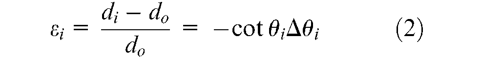
Mathar¹³ measured residual stresses by detecting the amount of strain release after drilling a small hole near a target point. However, since the original residual stress distribution may be influenced by the small hole, the accuracy was not high. Nowadays, residual stresses can be detected using non-destructive-testing (NDT) techniques, such as magnetic Barkhausen emission, ultrasonic wave detection or X-ray diffraction methods,^14–17 The X-ray diffraction method is selected in the present work and the measurement setup is shown in Figure 2. This method is accurate but has some limitations in selecting target points that don’t disturb the rotation of the probe. When a beam with wavelength $λ$ is transmitted through polycrystalline, a portion of the waves are diffracted and it can be expressed by Bragg’s law as

n λ = 2 d_{i} \sin θ_{i}

(1)

where $n$ is an integer, $θ$ is Bragg’s angle of plane and d is lattice spacing; see Figure 3. The lattice space d will be changed under residual stresses from the strain-free space d_o. Under the assumption of elastic and isotropic material, stress state can be calculated with the strain determined from equation (2). The orientation of the principal strain is decided by the geometry of the specimen. Some research groups have reported yield level residual stresses in the weld bead with this measurement technique.^15,16

ε_{i} = \frac{d_{i} - d_{o}}{d_{o}} = - \cot θ_{i} Δ θ_{i}

(2)

Figure 2.

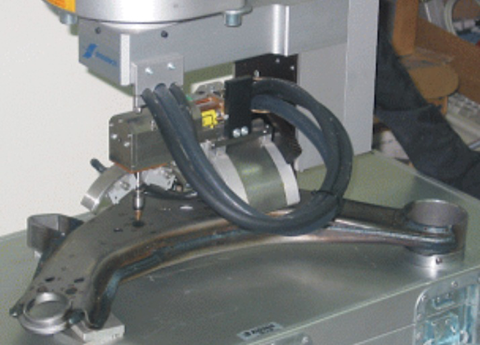
Residual stress measurement by the X-ray diffraction technique.

Figure 3.

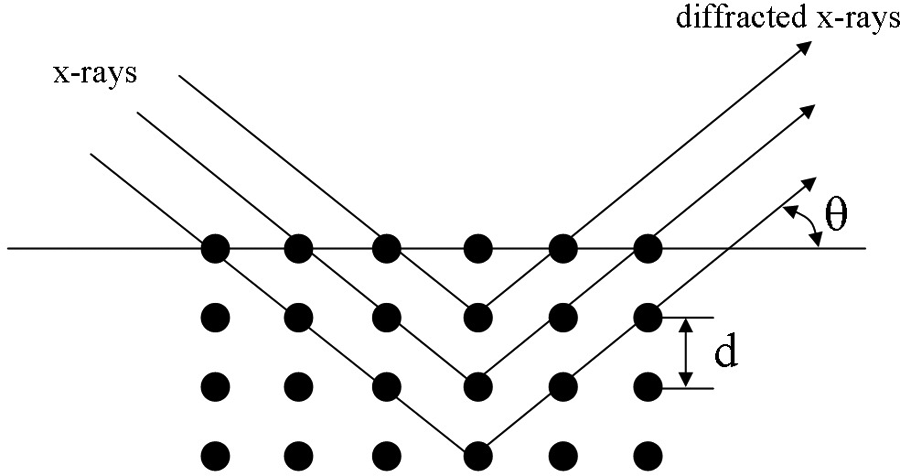
Schematic diagram to explain Bragg’s law.

Figure 4 is the measured residual stresses of the LCA at the indicated sections to the normal direction of each section. The nearest points to weld beads are measured since the bead is very rough and filler material has a different grain size to the panels. The residual stresses measured on the final product contain stamping and welding effects together. High tensile residual stress is detected at point 5, which is located in the heat affected zone in the wall area. Residual stresses in the heat affected zone are over 300 MPa and around 200 MPa at the other points. In order to verify the portion of stamping effects on the final stress distribution, a stamped panel before the welding process is picked out and stamping residual stresses are measured. The results are compared in Figure 5, which shows residual stresses increase after welding except the large deformed area owing to stamping. Since the drawing ratio of the LCA is small, stamping stress $σ_{XX}$ at the indicated local coordinate systems is below 100 MPa, except the large deformed region. It is expected that stresses at the corners will be higher than these results, but it was very hard to obtain results owing to the limitation of the equipment. Although the NDT technique is very useful for analyzing residual stresses, the method alone is not perfect owing to many constraints in the detection of stresses. Therefore, FE methods have been adopted to verify the residual stress distribution on the LCA.

Figure 4.

Residual stresses to the normal direction of the section on a final product: (a) section and measured points; (b) section A–A′; (c) section B–B′.

Figure 5.

Comparison between the stamping and coupled residual stresses to the direction X: (a) near the ball joint; (b) center, (c) near the G-bush.

Stamping simulations

In order to verify the work hardening effects on the weld residual stress distribution, stamping simulations have been carried out by LS-DYNA3D.¹⁸ Tools for stamping are modeled as represented in Figure 6(a). As the punch travels down with a prescribed velocity profile of which the maximum is 2 m/s, the sheet metal deforms in the die. Stresses in the blank are calculated with Mat_Transversely_Anisotropic_Elastic_Plastic constitutive model and the hardening curve of SAPH380 is represented in Figure 6(b). Hughes–Liu shell formulation with selective reduced integration is used. Explicit time integration with mass scaling is applied since the velocity is low enough to be assumed as quasi-static. A large tool load is applied to the binder to prevent wrinkling, and a static friction coefficient of 0.12 is used. The friction coefficient is a non-linear parameter affected by various forming conditions. In this study, an averaged value was used, which was measured when the viscosity is about 50 cSt and roughness is about 0.13 µm.¹⁹

Figure 6.

Tool setup for the stamping simulation.

To check the possibility of failure together with the accuracy of the simulation, simulated thicknesses at several points are compared to the measured results, as shown in Figure 7. The measured points are displayed in Figure 7(a) on each section with the simulated thickness distribution. Point 1 and point 3 are located at the wall with the indicated directions. Since the maximum thickness reduction in the simulation is below 20%, it can be inferred that failure does not occur in the panels. Maximum thickness reduction is observed at the point 1 or point 3 in the wall region in both the simulation and the measurement. Although the simulated thicknesses do not match exactly with the measurements, it is only within a 5% difference. Figure 8(a) shows deformed shapes and the effective stress distributions in panels obtained after the stamping simulation. Effective stress before springback is around 700 MPa at round corners in the wall and about 250 MPa at the other flat area.

Figure 7.

Comparison between numerically and experimentally obtained thicknesses: (a) simulated thickness distribution; (b) comparison at section A–A’; (c) comparison at section B–B’.

Figure 8.

Variation of the effective stress distribution (MPa).

The stress tensors obtained from stamping simulation satisfies the static equilibrium condition as long as the punch and the die keep contact with the blank, respectively. However, a new stress state should be calculated if the punch and the die are released from the blank. Elastic strains of the blank are released under the unloading condition, which results in a new stress equilibrium. The new stress state obtained after springback means the residual stress distribution of the stamping process. The amount of springback is calculated with the implicit algorithm to obtain stress states without dynamic oscillations. It can be seen in Figure 8(b) that the effective stresses are reduced particularly in the wall region. The size of elements used in the stamping simulation are much smaller than those of the welding simulations since, in order to discretize a die, at least four elements are necessary around each corner to prevent elements from kinks or sharp edges. For this reason, a mapping strategy should be used to consider the stamping results as initial conditions in welding simulation. In this study, thickness and effective plastic strain distribution are mapped onto the mesh for welding simulation, as showed in Figure 9.

Figure 9.

Thickness mapping onto a new mesh for weld simulation: (a) thickness distribution after stamping simulation; (b) thickness distribution for weld simulation after mapping.

Welding simulation

Heat transfer analysis

The second manufacturing step of the LCA is seam welding, which joins the upper and lower stamped panels by melting filler material. During the heating and cooling process, thermal deformation induces residual stresses in the work piece. Welding simulation is a non-linear thermo-mechanical coupled problem. As mentioned in the previous section, stamping effects will be included as initial conditions in the welding residual stress analysis. The temperature field is determined from heat transfer analysis and transferred into the analysis of thermal deformation. The governing equation for heat transfer is as

ρ c_{p} \frac{\partial T}{\partial t} = \frac{\partial}{\partial x_{i}} (k_{ij} \frac{\partial T}{\partial x_{j}}) + q in D

(3a)

k_{ij} \frac{\partial T}{\partial x_{j}} n_{j} = - k_{0} (T - g) + h on \partial D

(3b)

T = T_{0} at t = 0

(3c)

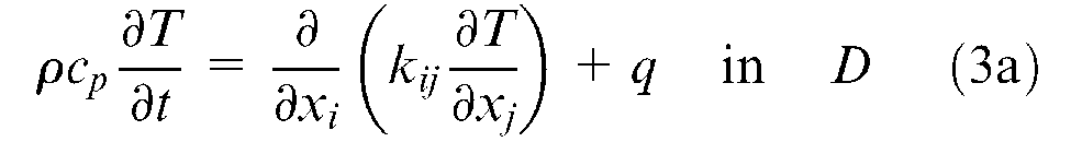
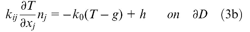
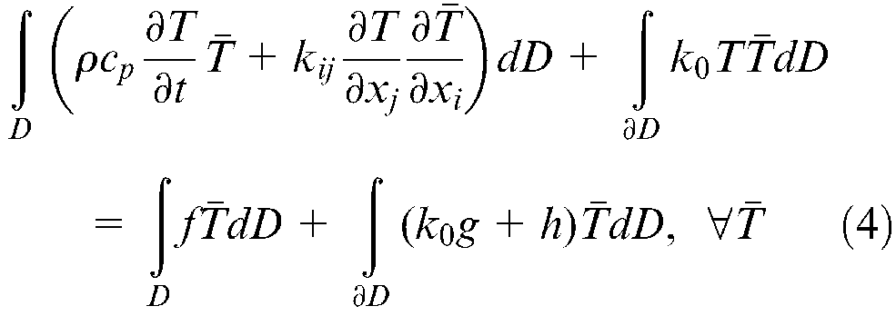
where ρ is density, c_p is specific heat per unit volume, k_ij is heat conductivity, q is heat generation, g and h are the specified temperature and the heat flux on some boundary surface. In welding problem, q is calculated with the electric power of a weld touch. A weak-form for FE analysis can be obtained as the principle of the first variation is applied to equation (3).

\int_{D} (ρ c_{p} \frac{\partial T}{\partial t} \bar{T} + k_{ij} \frac{\partial T}{\partial x_{j}} \frac{\partial \bar{T}}{\partial x_{i}}) dD + \int_{\partial D} k_{0} T \bar{T} dD = \int_{D} f \bar{T} dD + \int_{\partial D} (k_{0} g + h) \bar{T} dD, \forall \bar{T}

(4)

Many researchers have studied the modeling of the heat input from a weld torch. Gery at al.⁹ used a moving heat source based on Goldak’s double-ellipsoid heat flux distribution in order to predict transient temperature distribution at a butt joint. Goncalves et al.²⁰ studied thermal phenomenon in base metal during welding with optimization methods. Heat flux generated during the welding process was estimated and fusion efficiency was also estimated with consideration of the phase change and temperature-dependent thermal properties. Since it is known that residual stresses are influenced by the metallurgical phase transformation, thermo-elastic-plastic constitutive models are developed to investigate the change of yield strength owing to phase transformation.^21,22

In this study, heat flux from a weld torch is modeled with a simple equation in which the heat distribution effects are not included since the weld bead is narrow compared to the size of the LCA. A heat source calculated with equation (5) is applied to elements previously generated on weld beads.

q = η \frac{EI}{W_{elem_set} L_{elem_set}}

(5)

where $η$ is efficiency, E and I are voltage and current respectively, and W and L are width and length of an element set for weld bead. It was reported by Goncalves et al.²⁰ that the weld efficiency is 50 ∼ 60%, hence 0.55 is used in this study. Other parameters used in the welding simulation are summarized in Table 1.

Table 1.

Properties for the calculation of heat source for welding analysis.

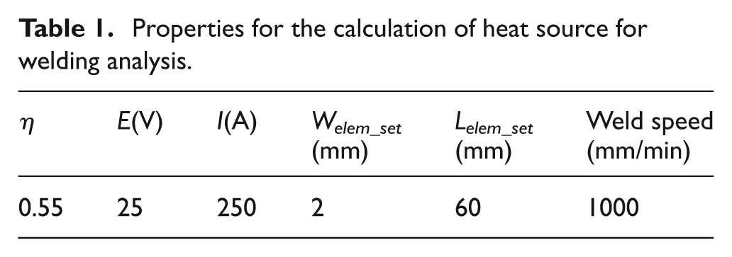
$η$	E(V)	I(A)	W_{elem_set}(mm)	L_{elem_set}(mm)	Weld speed (mm/min)
0.55	25	250	2	60	1000

It is difficult to automatically generate elements on weld beads as a weld torch moves along the beads in arbitrary 3D space. Therefore, weld elements are generated before the simulation and grouped every 60 mm to simulate the movement of a torch. Heat flux is given to the weld element groups with respect to the corresponding weld speed in Table 1. For example, if the length of a weld element group is 60 mm then heat is applied for 3.6 s. The profile is assumed as a square shape with short transient duration to avoid sudden heat loading as represented in Figure 10. This modeling scheme is relatively simple but reliable enough to study weld residual stress distribution. Since the maximum temperature in the weld bead reaches the phase change temperature, the latent heat effect has to be considered. The new specific heat is calculated with equation (6), which adds the latent heat to the original specific heat during the phase change duration

c_{p}^{'} = \frac{H_{L}}{T_{L} - T_{S}} + c_{p}

(6)

where $H_{L}$ is latent heat, $T_{L}$ is melting temperature and $T_{S}$ is solidifying temperature.

Figure 10.

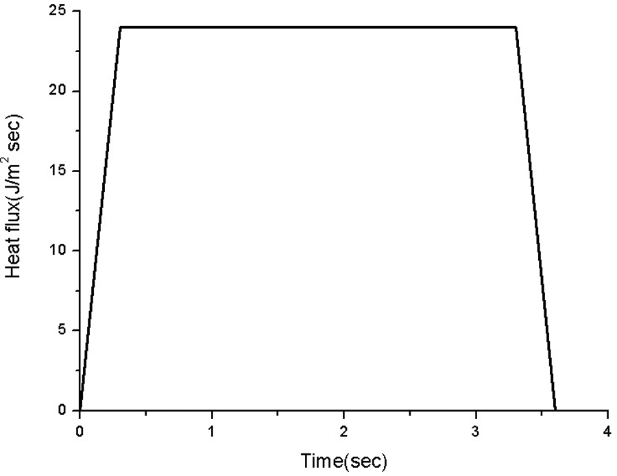
The profile for heat flux in a weld simulation.

Thermal deformation

The temperature field obtained from the heat transfer analysis is used in the thermal deformation analysis. The elastic co-rotational stress rate is determined from the total strain rate and thermal strain rate

σ_{ij}^{\nabla} = C_{ijkl} ({\overset{\cdot}{ε}}_{kl} - {\overset{\cdot}{ε}}_{kl}^{T}) + {\overset{\cdot}{θ}}_{ij} dT

(7a)

{\overset{\cdot}{θ}}_{ij} = \frac{d C_{ijkl}}{dT} C_{klmn}^{- 1} {\overset{\cdot}{σ}}_{mn}

(7b)

where ${\overset{\cdot}{ε}}_{kl}$ is total strain rate, ${\overset{\cdot}{ε}}_{kl}^{T}$ is thermal strain rate and $C_{ijkl}$ is the temperature-dependent elastic constitutive tensor. When treating plasticity, a return mapping algorithm is used. Thus the stresses are updated elastically and corrected on to a yield surface plastic integration path. The thermal strain rate can be expressed with the thermal expansion coefficient

{\overset{\cdot}{ε}}_{ij}^{T} = α \overset{\cdot}{T} δ_{ij}

(8)

During the welding process, high heat energy is transferred into the work piece and then cooled by ambient conditions; the material undergoes a wide range of temperature variations. In order to track the exact stress path, temperature-dependent material properties have to be used. The properties used in this study are represented in Figure 11. A LCA is made of sheet metal SAPH380, which is widely used in the automotive industry and temperature-dependent thermal properties can be found in literature.^23–25 Among the temperature-dependent properties, it was reported that the most important property in residual stress analysis is temperature-dependent yield strength.²⁵ However, it needs many kinds of experimental data on a wide range of temperatures. In this study, stress–strain relations on various temperatures are calculated with the Johnson–Cook model SAPH380, which is widely used in the modeling of strain-rate dependent material behavior. Coefficients of the model are obtained from quasi-static and high strain rate tensile tests up to several thousand per second. The heat generated from high strain rate deformation, over 10 °C/s, does not have enough time to transfer into the environment; it can be assumed to be an adiabatic condition. Internal plastic deformation energy is used to calculate temperature variations

\overset{\cdot}{T} = \frac{ξ}{ρ c_{p}} σ_{ij} {\overset{\cdot}{ε}}_{ij}^{p}

(9)

where $ξ$ is the thermal fraction of 0.8 to 0.9.²⁶ The stress–strain relations of SAPH380 in the form of the Johnson–Cook model¹¹ is

\bar{σ} = (265 + 580 {\bar{ε}}^{n}) (1.0 + 0.039 \ln \frac{\bar{\overset{\cdot}{ε}}}{{\bar{\overset{\cdot}{ε}}}_{0}}) (1 - T^{*^{0.43}}) (MPa)

(10a)

where T^* is the homologous temperature represented by

T^{*} = \frac{T - T_{room}}{T_{melt} - T_{room}}

(10b)

where T is the temperature of the specimen, and T_melt is the melting temperature of the specimen. The first term in equation (10a) is the strain hardening term, the second is the strain rate hardening term, and the third is the thermal softening term. The calculated stress–strain curves with the Johnson–Cook model, after omitting the second term, are shown in Figure 12.

Figure 11.

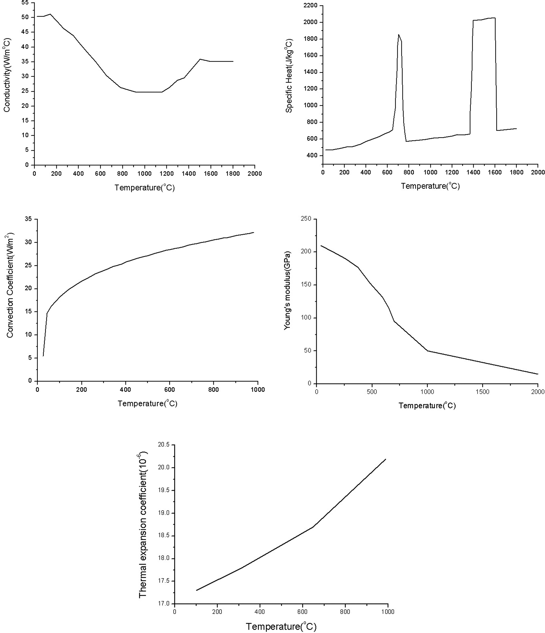
Temperature-dependent material properties for a thermal deformation analysis.

Figure 12.

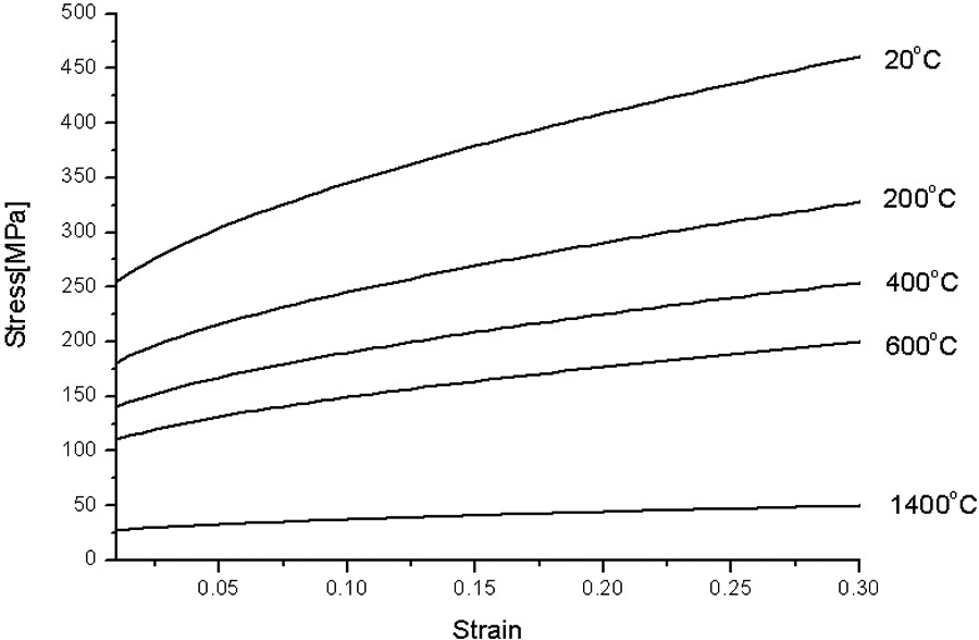
Stress–strain curves at the various indicated temperatures.

Residual stress analysis

An FE model for the analysis of thermal deformation is shown in Figure 13 with boundary conditions. A total of 19 element groups are modeled in the weld bead and the first two of them are displayed as an example. The temperature distribution calculated with the moving heat source model is shown in Figure 14. The maximum temperature is over 1000 °C at the weld bead and several hundred degrees at the heat affected zone. In order to verify the suitability of assumptions mentioned before, temperature measurements have been performed with two samples. Four thermo couples are attached respectively at each sample; see Figure 15. It is not possible to attach a thermo couple directly on the weld bead in order not to disturb the movement of the weld torch. Points on the heat affected zone are selected instead, which are located at the middle of the vertical panel wall. Figure 15 is the experimental setup and measured temperature profiles. Maximum temperature reaches 400 °C at a close point to the bead. At far points from the bead, around 100 °C is taken owing to the heat conduction from the weld bead.

Figure 13.

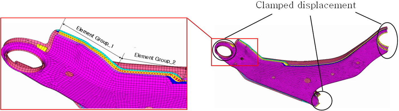
Finite element mesh representing weld element groups for a weld simulation.

Figure 14.

Temperature distributions with a moving heat source: (a) after 3.1 s; (b) after 7.1 s; (c) after 21 s; (d) after 24.4 s.

Figure 15.

The results of temperature measurements: (a) sample I; (b) sample II.

Simulation results are compared with the test results in Figure 16, which shows good correlations. The simulated initial slopes are much steeper than those of the test results but temperature peaks are quite similar in both cases. Although the heat generation is considered as a group-wise event in the present simulation, the total amount of the heat input is the same in both cases. However, the heating rate is much faster in the case of the simulation. Thus, the initial slopes of the temperature histories are different but temperature peaks are similar to each other. Since thermal strain rate is the function of the temperature rate, the slopes of the curves in Figure 16 relate to the thermal strain rate. The calculated thermal stress rate during heating is larger than that of the experiment. The cooling rate is also much faster in the case of the simulation in the early state, but reaches equilibrium at almost the same time. It means the thermal stress rates during cooling become similar with elapsed time. The final equilibrium is achieved after one hour and, hence, the effects of the difference in initial slopes can be neglected. Temperature calculations by the group-wise heat source model is relatively simple but gives quite a good result.

Figure 16.

Comparison between experimentally and numerically obtained temperature histories: (a) measurement; (b) simulation.

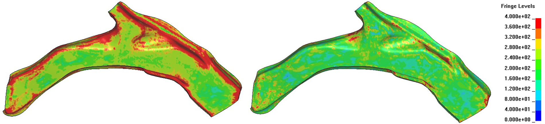
Two weld simulations have been performed for the verification of stamping effects. The first one is performed without any stamping effects. The second one uses stamping results as initial conditions. Figure 17 is the effective stress distributions of the two simulation results. High effective stresses at the wall can be observed only in the case of considering the stamping effects. Since effective stresses after springback are not as high as displayed in Figure 17(b), the high stress distribution at the wall is representing the sequential process effects of stamping and welding.

Figure 17.

Comparison of the weld residual stress distributions: (a) without stamping effects; (b) with stamping effects.

In order to scrutinize the stamping effects on welding residual stress, point 1 and point 4 are selected, which are marked on the upper-left side of Figure 15. Figures 18 and 19 are time histories of effective stresses, temperatures and plastic strains obtained from simulations at the selected points. Figure 18 gives the results of the welding simulation without stamping effects and Figure 19 gives the coupled simulation results. The effective stresses in both cases begin to increase before the heat source arrives at point 1 owing to global deformation of the LCA. As the heat source comes close to the point 1, temperature quickly increases while stress goes down owing to thermal softening. After the temperature reaches its maximum value, cooling begins and the stress starts to increase again. Plastic strain at point 1 increases faster during heating and almost stays constant during cooling. Since the thermal properties for the temperature calculation are not influenced by the stamping effects, temperature changes are the same regardless of the stamping effects. However, the amount of a stress drop during heating depends on the initial state of stress, strain and the variation of temperature. Actually, the temperature histories are identical in both cases, thus the amount of stress drop is decided by the yield surface at the maximum temperature as well as the initial stress state. From both figures it can be seen that the stress drop is larger when the stamping effects are included in the simulation. However, the stress increase during cooling is almost the same in both cases because the variation of temperature is identical. As a result, large weld residual stresses are obtained when the stamping effects are included but not as large as the linear summation of weld and stamping residual stresses (Figure 20). The stamping or welding simulation alone cannot predict the large wall stress generation on the final product but the sequential non-linear simulation successfully predicts the high stresses at the wall region. Figure 21 shows the flowchart of the entire process from the simulation of stamping and welding to the experimental validation.

Figure 18.

Time histories of weld simulation results without stamping effects at the indicated points: (a) effective stress and temperature histories; (b) plastic strain histories.

Figure 19.

Time histories of stamp welding coupled simulation results at the indicated points: (a) effective stress and temperature histories; (b) plastic strain histories.

Figure 20.

Stress distribution after springback $(σ_{XX})$ .

Figure 21.

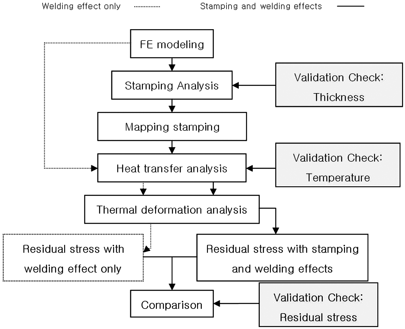
Flowchart of the simulation and experiments.

Conclusions

Residual stress distribution in a LCA is calculated by FE methods. The stamping or welding simulation alone cannot predict the large wall stress generation on the final product; however, the sequential non-linear simulation (i.e. welding simulation) with consideration of the stamping effect was found to show excellent predicts of the high stresses at the wall region. The neutron diffraction method is used to qualitatively investigate the residual stress level on the real product. High residual stresses at the wall region near the weld beads are detected. The measurement also reveals that the residual stresses in the stamped panels increase after welding in a non-linear manner. For the welding simulation, a simple modeling method is proposed with several assumptions and verified with test results. A moving heat source is considered by a group-wise heat input. Temperature-dependent stress–strain relation is obtained from the Johnson–Cook model SAPH380, which is well known for strain-rate-dependent material behavior. The test results indicate the simulation method leads to different temperature rates in early state, but maximum temperatures and cooling rates are almost similar. Stamping effects, such as uneven thickness distribution and work hardening, are obtained with an incremental simulation method and applied to weld residual stress analysis as initial conditions using a mapping method.

Footnotes

This research received no specific grant from any funding agency in the public, commercial, or not-for-profit sectors

References

Lee

Biglari

Wimpory

. Treatment of residual stress in failure assessment procedure. Eng Fracture Mech 2006; 73: 1755–1771.

Hiroyuki

. The effect on fatigue life of residual stress and surface hardness resulting from different cutting conditions of 0.45%C steel. Int J Mach Tools Manuf, 2005; 45: 131–136.

Han

Young

Chrysanthou

. The effect of pre-straining on the mechanical behaviour of self-piercing riveted aluminium alloy sheets. Mater Des 2006; 27: 1108–1113.

Huh

Kim

. Crashworthiness assessment of front side members in an auto-body considering the fabrication histories. Int J Mech Sci 2003; 45(1): 1645–1660.

Chen

Liu

Knoerr

. Residual forming effects on full vehicle frontal impact and body-in-white durability analysis. SAE Technical Paper, 2002; 2002-01-0640.

Sala

. A numerical and experimental approach to optimize sheet stamping technologies. Part I: mild steel press-forming. Mater Des 2001; 22: 285–298.

Holmberg

Thilderkvist

. Influence of material properties and stamping conditions on the stiffness and static dent resistance of automotive panels. Mater Des 2002; 23: 681–691.

Klobcar

Tusek

Taljat

. Finite element modeling of GTA weld surfacing applied to hot-work tooling. Computational Mater Sci 2004; 31: 368–378.

Gery

Long

Maropoulos

. Effects of welding speed, energy input and heat source distribution on temperature variations in butt joint welding. J Mater Processing Technol 2005; 167: 393–401.

10.

Umbrello

M’Saoubi

Outeiro

. The influence of Johnson–Cook material constants on finite element simulation of machining of AISI 316L steel. Int J Mach Tools Manuf 2007; 47: 462–470.

11.

Huh

Kang

Han

. A tension split Hopkinson bar for investigating the dynamic behavior of sheet metals. Experimental Mech 2002; 42(1): 8–17.

12.

Huh

Lim

Kim

. Formability of the steel sheet at the intermediate strain rate. Key Eng Mater 2004; 274(1): 403–408.

13.

Mathar

. Determination of initial stresses by measuring the deformation around drilled holes. Trans ASME, Iron & Steel 1934; 56: 245–249.

14.

Moorthy

Shaw

Hopkins

. Surface and subsurface stress evaluation in case-carburised steel using high and low frequency magnetic Barkhausen emission measurements. J Magnetism Magnetic Mater 2006; 299: 362–375.

15.

Larsson

Holden

Bourke

MAM

. Measurement and modeling of residual stress in a welded Haynes 25 cylinder. Mater Sci Eng A 2005; 399: 49–57.

16.

John

WHP

Anna

Suraj

. Residual stresses measurement by neutron diffraction and theoretical estimation in a single weld bead. Int J Pressure Vessels and Piping 2006; 83: 381–387.

17.

Chen

Kovacevic

. Finite element modeling of friction stir welding-thermal and thermo-mechanical analysis. Int J Mach Tools Manuf 2003; 43: 1319–1326.

18.

LS-DYNA, Version 970 User’s Manual.

19.

Lee

Keum

Wagoner

. Modeling of the friction caused by lubrication and surface roughness in sheet metal forming. J Mater Process Technol 2002; 130–131: 60–63.

20.

Goncalves

Vilarinho

Scotti

. Estimation of heat source and thermal efficiency in GTAW process by using inverse techniques. J Mater Process Technol 2006; 172: 42–51.

21.

Kim

. Numerical implementation of a thermo-elastic-plastic constitutive equation in consideration of transformation plasticity in welding. Int J Plasticity 2005; 21(7): 1383–1408.

22.

Deng

Murakawa

. Prediction of welding residual stress in multi-pass butt-welded modified 9Cr.1Mo steel pipe considering phase transformation effects. Computational Mater Sci 2006; 37: 209–219.

23.

Huh

Kang

. Electro-thermal analysis of electric resistance spot welding processes by a 3-D finite element method. J Mater Process Technol 1997; 63: 672–677.

24.

Han

Zhao

. Dynamic simulation of the temperature field of stainless steel laser welding. Mater Des 2007; 28: 240–245.

25.

Zhu

Chao

. Effects of temperature-dependent material properties on welding simulation. Comput Struct 2002; 80: 967–976.

26.

Mason

Rosakis

Ravichandran

. On the strain and strain rate dependence of the fraction of plastic work converted to heat; an experimental study using high speed infrared detectors and the Kolsky bar. Mechan Mater 1994; 17: 135–145.

Analysis of coupled residual stresses in stamping and welding processes by finite element methods