
Abstract
By control of their constituents, interfaces and architectures, composite materials can display a much broader suite of beneficial material properties than is possible for single-phase materials. Furthermore, advanced manufacturing techniques are increasing the freedom to operate of composite designers. While much can be achieved with idealised models of composites, models are needed that more accurately reflect the non-ideal placement of reinforcement, matrix-free regions and manufacturing defects that occur in practice. At the same time, imaging techniques, and X-ray computed tomography in particular, have radically increased the level of information that can be obtained in three dimensions and over time about real composite microstructures, both about the as-manufactured condition and their behaviour in-service. This review considers all aspects of image-based modelling of composite materials across the length scales. It also discusses establishing the appropriate constitutive equations for deterministic and stochastic (e.g., fibre fractures) elements of behaviour, as well as methods for validation. A range of actual and potential applications from the literature are showcased throughout. It explores approaches to bridging the scales and techniques, such as surrogate and homogenised models, to ensure models are computationally feasible. It covers a wide range of composites, spanning polymer, metal and ceramic matrices, continuous and short fibres, as well as particulate reinforcements. It also briefly extends to how such approaches can be applied to other ‘composite’ systems, such as concrete and hard metals. Overall, this is a one-stop review for those considering multiscale modelling of composites based on realistic, often multiscale, composite architectures.
Keywords
Introduction
Composite materials offer almost limitless scope for the design of material architectures that bring together the attributes of different phases to deliver properties that can be anisotropic, and that can be varied locally to optimise performance across a component or structure. In addition, the various interfaces within a composite can be controlled to deliver functionalities not even possessed by the constituents that make them up (e.g., tough ceramic composites from brittle constituents). Nowhere is this design freedom more evident than in nature, 1 where composites rule supreme, delivering a range of useful properties from quite ordinary constituents through complex hierarchical structures from the Bouligand structures giving rise to the iridescence of beetles, 2 to the interdigitated layers comprising co-oriented needles, plates, and a polycrystalline matrix conferring upon sea urchin teeth the self-sharpening wear resistance needed to grind rocks. 3
This freedom to operate has yet to be widely explored in manufacturing despite the need for composite materials across aerospace, marine and many other sectors and the advent of ‘additive’ manufacturing methods that offer greater design flexibility. This is in part because we do not have the models needed to explore this space in detail. This problem is compounded by our reliance on an extensive and time-consuming testing pyramid (see Figure 1) requiring expensive sets of tests across the various length scales. Consequently, if we are to expand the use of composite materials and explore the opportunities they present, we need to enhance modelling capability across all length scales. This requires a digital twin for both composite manufacturing and for predicting composite performance. Many of the larger length scales can be modelled by finite element modelling, although the question of manufacturing defects and uncertainty require further attention. Here, we focus primarily on the scales relevant to modelling at the coupon scale. According to the reinforcement type and composite architecture, these range from modelling the matrix, reinforcement and interface, to the tow (fibre bundle level), to the textile or laminae scale to the coupon scale.
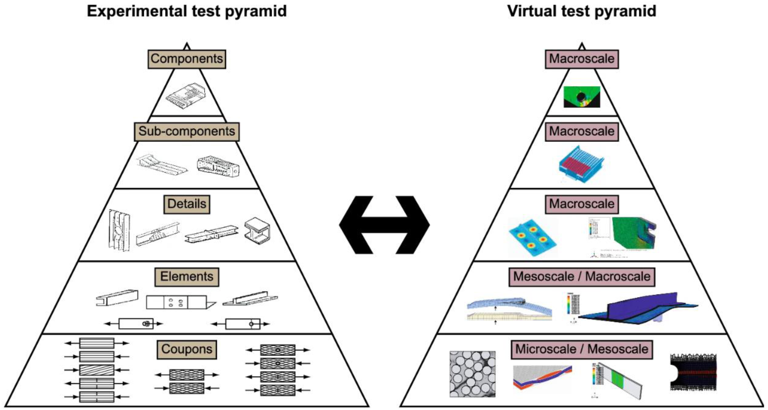
To lower the cost of composite manufacturing and certification, the multiscale experimental test pyramid needs to be complemented by its digital twin. 4
The simplest approach to composite modelling is to try to capture the essence of the composite without considering the separate phases explicitly through a continuum model (as illustrated in Figure 2(b)). In this case, the influence of the reinforcement is described using continuum composite laws. These can include continuum damage accumulation parameters. To capture the influence of the interface, the phases must normally be included explicitly, and the computationally simplest way of doing this is via an idealised unit cell taken to repeat many times throughout the composite (see Figure 2(c)). In the case illustrated, the properties of the ‘matrix’ could be adapted to consider the effect of the fine scale pores visible in Figure 2(a). As to whether the simplest unit cell is sufficient may depend on whether volume-averaged properties, such as stiffness, are required or properties more dependent on local aspects, such as damage or fracture. It can also depend on whether composite variability and/or manufacturing defects need to be incorporated into the representative volume element (RVE). In many cases, the RVE, or sometimes the statistically equivalent RVE, 5 which is the smallest volume that must be modelled to accurately capture the behaviour of interest, must be considerably bigger than an idealised unit cell. Either synthetic or imaged-based RVEs of increasing complexity and size can be employed (see Figure 2(d)–(f)), but at the cost of significantly increased computational demands. Often, 3D image-based models are generated from 2D Scanning Electron Microscope (SEM) images such as that in Figure 2(a), although 3D models based on X-ray Computed Tomography (X-CT) are becoming more common. Indeed, it is sometimes referred to as X-ray tomography aided engineering.
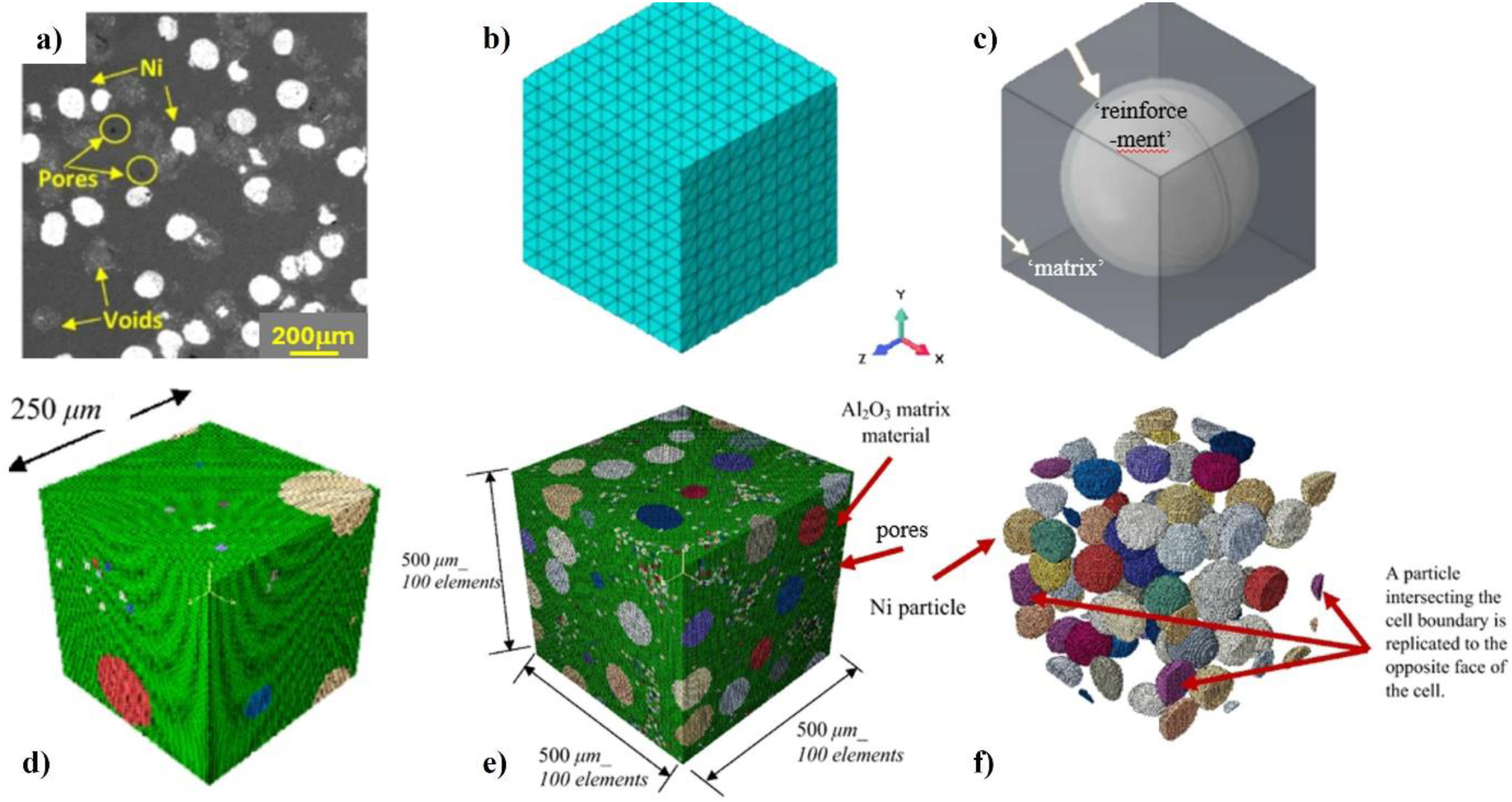
(a) A 2D SEM image of a sintered Ni particle/ Al2O3 matrix composite, (b) a continuum representation exploiting a composite model, (c) a simple idealised unit cell, (d) small (125,000 elements) and (e) larger (1 million elements) representative volume elements that capture many features of the composite, and f) periodic nature of RVEs created by DREAM.3D from the 2D image in (a) (images from 6 ).
In practice, a combination of these approaches is often employed in multiscale modelling (see sub-section: Multiscale modelling). For instance, an image-based model can be used to capture the defects and arrangement of fibres within a laminate, while a continuum model is used to carry these properties over into a laminate and then to the component scale.
This review covers all the processes needed to construct, apply and validate image-based modelling from the capturing of image data, building the models and the underlying constitutive equations to their application in manufacturing and the prediction of in-service properties. It is relevant to the modelling of a wide range of reinforcement morphologies. This includes the particulate reinforcements typical of discontinuous metal matrix composites, hard metals (cemented carbides) and cementitious materials (e.g., concrete). While in some cases, the level of particulate reinforcement is varied through the component, generally, such composites do not require consideration of any longer microstructural length scales, and so image-based models can be relatively small. Polymer-matrix short-fibre systems are attracting increasing interest due to their ease of manufacture and recycling, as well as their ability to use recycled fibres. These introduce the complexity of anisotropy. Much of the review is focused on long fibre composites, mainly polymer and ceramic matrix composite systems. The fibres can be arranged in the form of various textiles as well as in laminae, resulting in the need to produce complex multiscale models. Layered composites building on natural examples, such as nacre, are also being explored as a means of making tougher high-temperature ceramic composites, while structured (lattices) and unstructured (foam) porous materials can be thought of as air composites and are also benefiting from microstructural design through image-based modelling. Some of these composite systems are discussed in the Applications p section.
Capturing image data
The first step of image-based modelling is to collect realistic images that capture the key features at the appropriate scale(s). This could be of the whole component or only a small sample that is needed to generate an RVE to form an image-based sub-model. 7 X-ray imaging methods can now provide 3D images of unparalleled detail, 8 but in some cases, it is sufficient, simpler, and more cost-effective to capture 2D images and to use these as the basis for 3D modelling.
2D microscopy of composites
Much of what we have learnt about structure/property relationships in composite materials has been gained from optical or scanning electron imaging of composite sections. 9 Great care must be taken when sectioning to avoid introducing artefacts. Two-dimensional imaging methods are generally much cheaper than their 3D equivalents, and one can examine large areas at high resolution to help ensure their representativeness. Three-dimensional quantities such as fibre orientation 10 and length 11 distributions can be obtained from these sections, often by analysing images taken at multiple depths, or in perpendicular directions at selected locations by a process called stereology, which has been reviewed for composites by Lukas and Chaloupek. 12
In some cases, 2D image-based models are sufficient, for example when modelling well-aligned long fibre materials or isotropic particulate materials such as concrete. 13 In other cases, sufficiently realistic 3D images can often be inferred directly from the 2D images. Indeed, some software, such as DREAM 3D 14 (now DREAM3D-NX), can create realistic 3D microstructures from quantities (e.g., particle size, shape distribution and the radial distribution function) obtained directly from 2D images, as shown in Figure 2. One of the first codes to do this was CEMHYD3D, 15 designed to create 3D cementitious RVE microstructures. Recently, a generative machine learning algorithm called sliceGAN 13 has been developed to create realistic 3D images from a single 2D slice in cases where the properties are isotropic (Figure 3(b)), or from two or more perpendicular planes when they are not (Figure 3(c)).
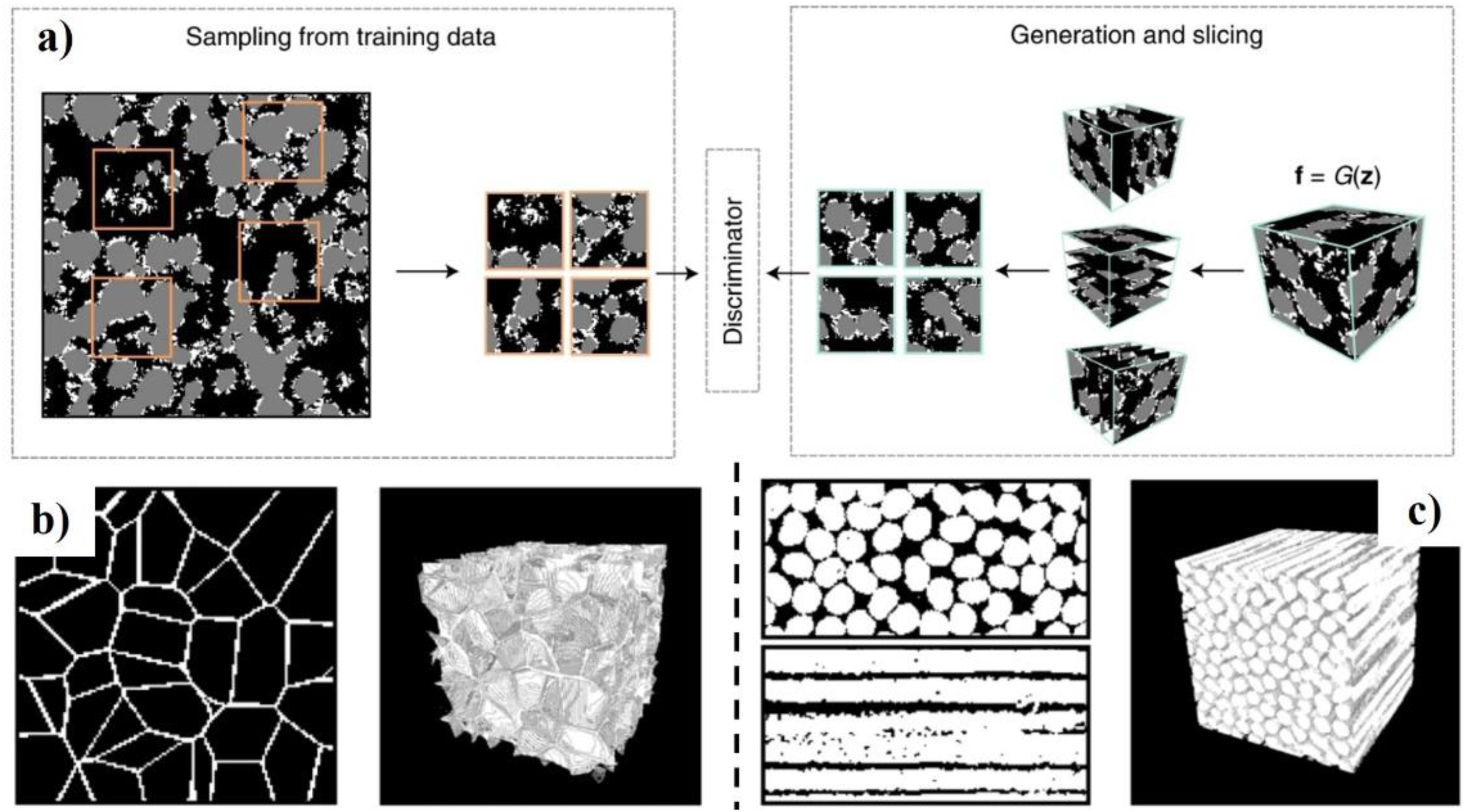
Inferring 3D images from a 2D image, (a) first, real images are sampled from the 2D training sample, a fake volume is then generated and sliced along x, y and z. This yields a compatible pair of datasets, which can both be fed to a 2D discriminator. Exemplar binarised training data (left hand image) and inferred 3D volume (right hand image) for (b) a cellular foam and (c) a fibre composite. 13
It is also possible to combine serial sectioning with scanning electron or optical imaging to create 3D image volumes using ion beams (100 μm sized volumes), 16 laser beams (mm volumes)17,18 or mechanical sectioning methods 19 (10–100 s of mm volumes). While such methods can be used to create an image stack sufficient to create an image-based sub-model of, say, the fibres within a laminate, only mechanical sectioning is really of a length scale suited to creating meso- or macroscale models of woven or composite laminate architectures. 20
X-ray computed tomography (X-CT)
With the increasing demand for real-time 3D characterisation and advancements in spatial resolution, X-CT has emerged as a powerful tool for multiscale imaging (micro-, meso- and macroscale) of composite structures, manufacturing defects and in-service damage.21–23 Figure 4(a) shows how a series of X-ray radiographs, or projections, of a sample acquired as it is rotated can be processed using a reconstruction algorithm to obtain a 3D image of the specimen. We usually distinguish two kinds of tomography: laboratory (or lab) tomography, using an X-ray tube as source, and synchrotron tomography using a synchrotron light source. Lab sources generally provide a conical beam containing a range of X-ray energies depending on the accelerating voltage and target material, while synchrotron sources usually provide a parallel beam that is more brilliant, enabling significantly shorter acquisition times.
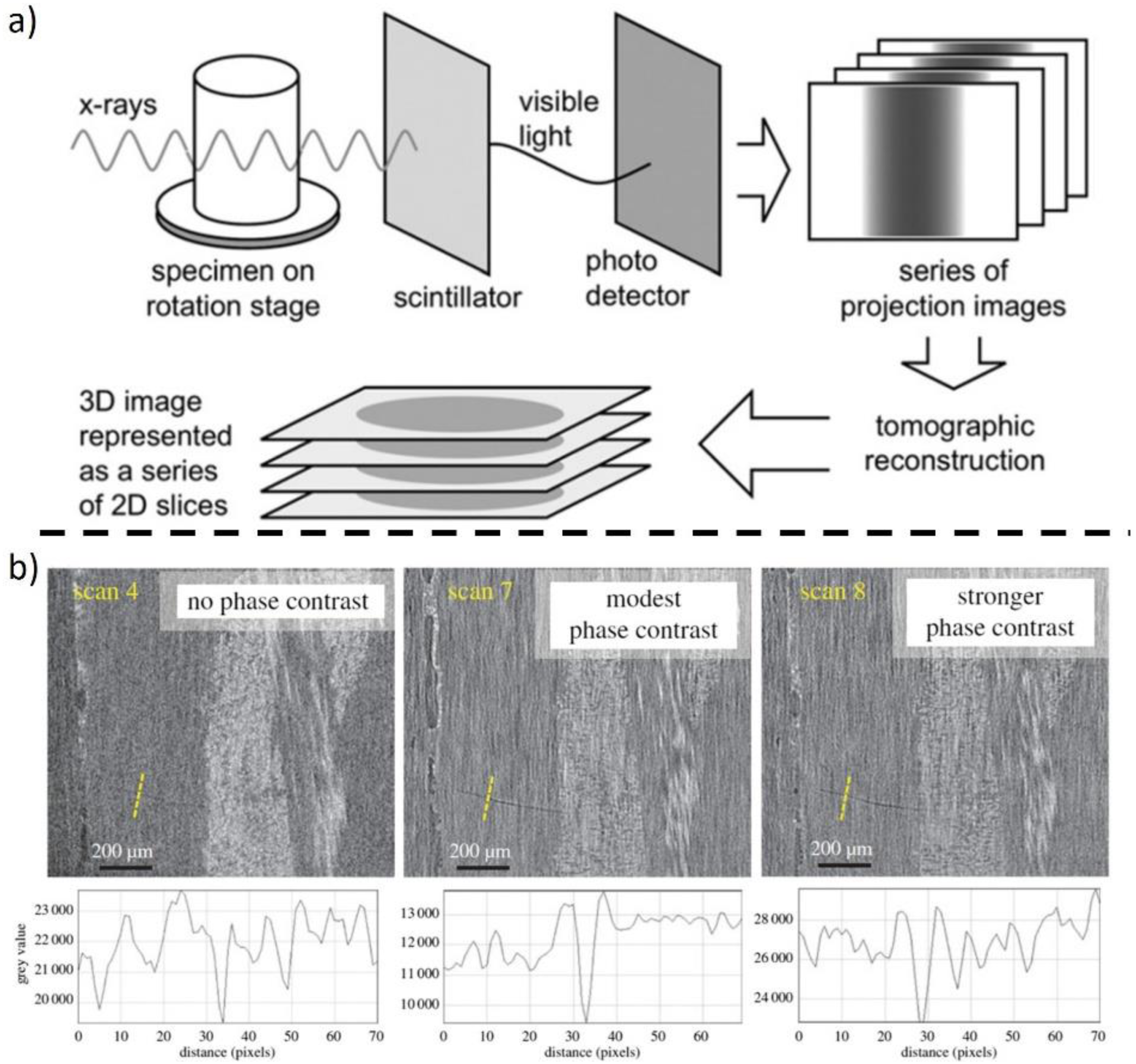
(a) schematic illustrating the X-CT image acquisition process 24 and (b) three virtual X-CT slices corresponding to the same plane in a 3D glass-fibre woven composite without phase contrast, with modest in-line phase contrast and with stronger phase contrast. The grey scale line profiles correspond to the dashed yellow line. 25
Two contrast modes are possible in conventional X-CT: a) absorption (or attenuation) contrast, which is the most common and is available with both laboratory and synchrotron sources; and b) phase-contrast, which requires a coherent beam and usually requires a synchrotron source. 8 They derive from the imaginary (β) and real (δ) parts of the refractive index, n, which is usually written as,

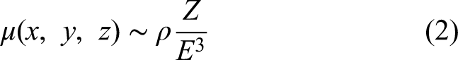
Absorption contrast results from the reduction of intensity of X-rays as they pass through the sample constituents, absorption tomography is then an image of the local attenuation coefficient μ(x, y, z). The attenuation coefficient broadly varies (neglecting absorption edges) as8,23:
X-ray phase contrast 8 imaging is particularly useful for weakly attenuating materials, 21 as material interfaces can be enhanced by detecting the phase shifts. Several experimental approaches exist for detecting phase shifts. The simplest is propagation-based phase-contrast imaging (also called in-line phase contrast imaging),26,27 which arises when the beam is sufficiently coherent, usually using synchrotron radiation, and the sample-to-detector distance is large enough (see Figure 4(b)). Phase contrast imaging provides enhanced edge definition and improved feature detectability in carbon fibre-reinforced polymer (CFRP) composites, as shown in Figure 4(b). In practice, the measured image is a combination of phase and absorption contrast, their contribution can be tuned a posteriori using filters, such as a Paganin filter. 28
The spatial resolution of X-CT images is generally around 2–3 pixels. 21 For a given pixel size, the field of view is limited by the size of the detector (typically a 4–12 mega-pixel array). However, by stitching projections or volumes together, the field of view can be increased (at the cost of a higher acquisition time). 29 In many cases, the main limitation is not the acquisition of the images, but the processing of the huge volume data. Given the multiscale nature of many composites, this limitation must be borne in mind alongside the computation limits when choosing what aspects of the composite require image-based methods, e.g., the arrangement of the individual fibres, the fibre tows, or the individual laminates.
As illustrated in section: Applications, a key advantage of X-CT over destructive sectioning is that it allows repeated 3D imaging to follow structural changes during manufacturing, or in response to in-service environments or loading histories. This can be done by continuous capture whereby the sample is continuously rotated relative to the X-ray source, or by in-situ or ex-situ time-lapse imaging to monitor longer timescale events. In general terms, synchrotron beamlines are better suited to short timescale, microscale, small sample studies, while lab sources are better suited to longer timescale and larger specimen/component studies. In both cases, this means that X-CT is not just an excellent means of setting up image-based modelling strategies but also for validating the predictive capability of the resulting models (see sub-section: Validation with experimental results).
Small-angle scattering tensor tomography
It is often not feasible to image individual fibres at sufficient resolution, or with sufficient contrast, by X-CT to segment them individually. In such cases, indirect methods come into play, for example exploiting two-dimensional small-angle X-ray scattering (SAXS) to reveal microstructural anisotropy.30–34 One means of doing this is to use an array of circular gratings32,35 (see Figure 5(a)), enabling anisotropic scattering information to be extracted at each image pixel by measuring the change in the circular fringes before and after inserting the sample into the beam path. After reconstructing the local 2D small-angle X-ray scattering signal, scattering tensors describing the local 3D scattering character of each voxel within the sample33,34 can be computed from which the degree of fibre orientation in 3D can be inferred,32,35 as shown in Figure 5.
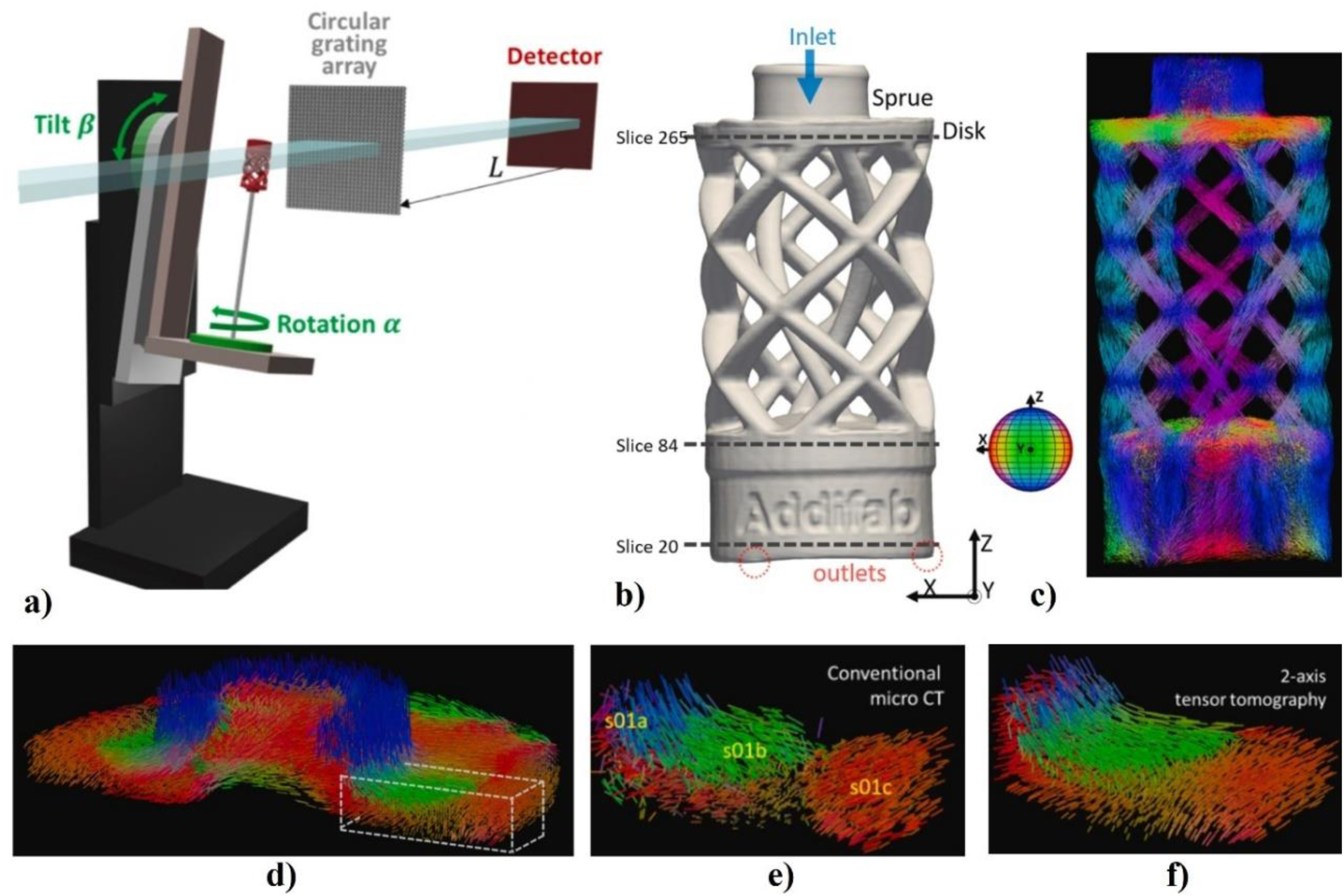
(a) schematic of small-angle X-ray scattering (SAXS) tensor tomography setup, (b) carbon fibre-reinforced freeform injection moulding, (c) preferential orientation of the fibres in each voxel, (d) 3D tensor tomography view around the inlet sprue region with the dashed box showing the location of the magnified region of interest acquired by (e) conventional X-CT image showing the orientation of the actual fibres and (f) tensor tomography showing the inferred orientations. 34
Building image-based models
Except when modelling the whole component, a key question is how big a region is needed to represent the composite at the length scale of interest. Computational complexity and imaging limits typically prohibit image-based modelling across all three length scales (micro-, meso- and macroscale) simultaneously. As a result, hybrid approaches combining image-based models with continuum models are common. In this context, it is critical to choose a 2D area, or a 3D image volume, that is large enough to be representative of the structural scale of interest, but not so big that the calculation is computationally infeasible. A lot of research has been undertaken to determine how big the RVE should be.36,37 In this respect the definition proposed by Drugan and Willis 38 is helpful: ‘‘It is the smallest material volume element of the composite for which the usual spatially constant (overall modulus) macroscopic constitutive representation is a sufficiently accurate model to represent mean constitutive response’’.
In this section, we consider the image processing (sub-section: Segmenting images into distinct phases) and meshing and mapping (sub-section: Turning phases into finite element meshes) that are key elements of the image-based modelling workflow shown in Figure 6 before going on to look at the assignment of properties to the constituents in section: Constitutive equations.
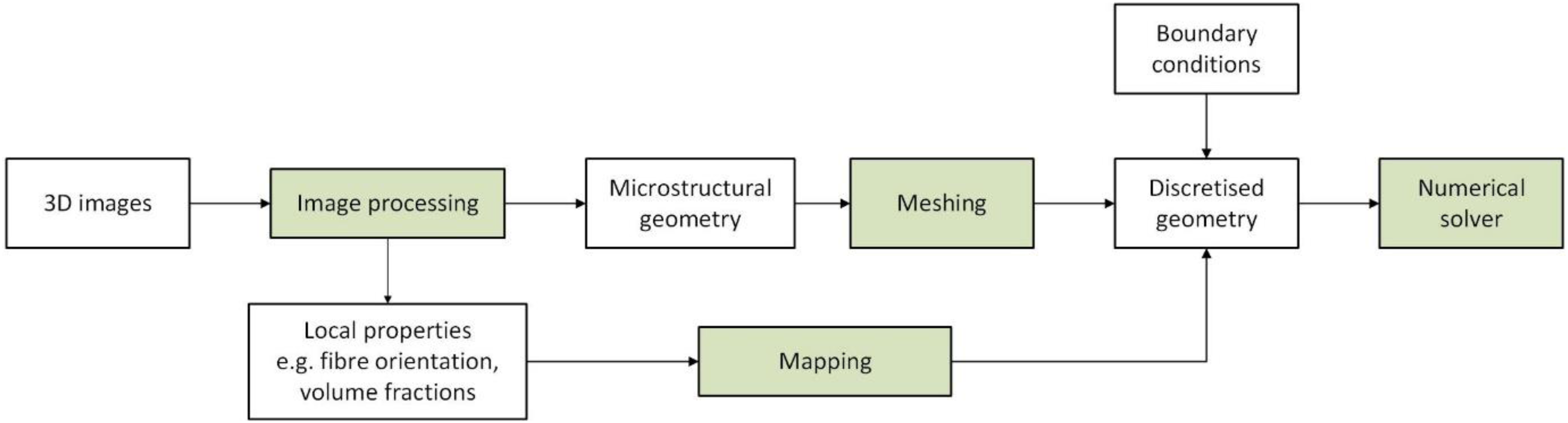
Typical workflow for image-based simulation. The green boxes indicate the processing steps that may involve dedicated development for different material systems.
Segmenting images into distinct phases
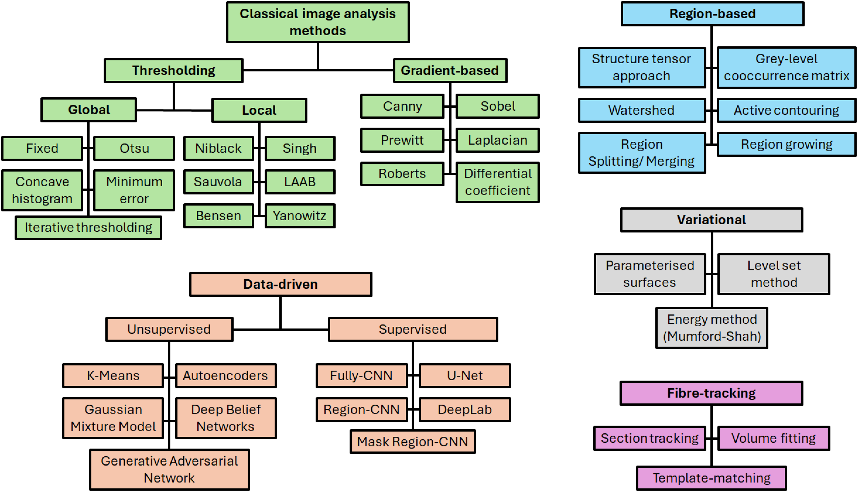
A key aspect when using image-based data is the need to assign (or segment) different regions of the images to specific phases or features e.g., matrix, voids/pores and yarns/fibres. This can be achieved through a number of approaches under the broad theme of segmentation. The simplest and still the most widely used method, global thresholding, is to assign pixels to different phases according to specific greyscale ranges. This method is prone to noise in the image, changes in illumination across the image volume or between different X-CT scans and it cannot accurately segment objects or regions that have overlapping intensity values. Various more sophisticated segmentation approaches have been developed,39–41 as shown in Figure 7 and Table 1. We classify them into the following categories: classical approaches based on intensity and gradient such as thresholding and edge detection algorithms, region- and feature-based algorithms, variational and model-based methods, data-driven methods and fibre tracking methods. Often, a complex segmentation problem requires a combination of these methods to achieve satisfactory results. A range of software has been developed for segmentation and meshing of X-CT images of composites: the most widely used of these are listed in Table 2.
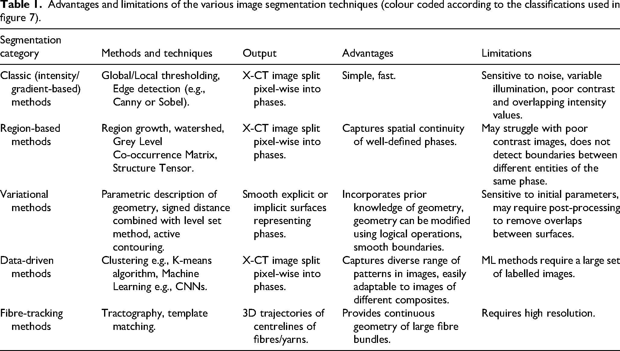
Advantages and limitations of the various image segmentation techniques (colour coded according to the classifications used in figure 7).
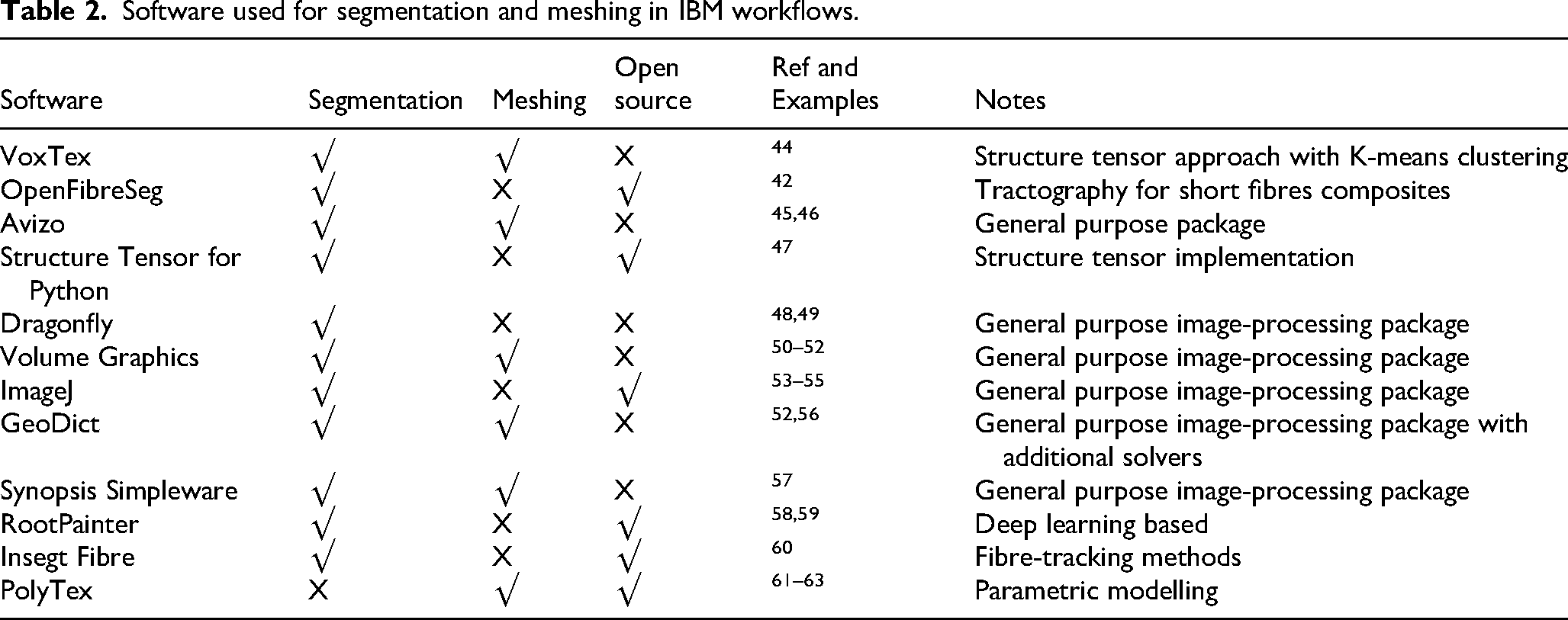
Software used for segmentation and meshing in IBM workflows.
Classical segmentation approaches
A classical computer vision approach to segmentation is to use thresholding and/or edge detection algorithms.
Region-based methods
This class of methods aims to divide an image into regions based on similarity criteria, such as texture or local fibre orientation, by grouping pixels into regions based on their similarity and then merging or splitting regions until the desired level of segmentation is achieved. One such method is watershed, a classical computer vision algorithm that splits the regions using gradient of the image to construct edges between the regions, which is still used in conjunction with more advanced techniques.
One other method is the grey level co-occurrence matrix, a statistical method which counts frequency of pairs of pixels with given intensities and spatial positions appearing in an image. The homogeneity metric, which can be easily derived from the grey level co-occurrence matrix, can be used to separate yarns in a dry fibre textile 69 but may struggle when applied to carbon fibre composites having a high fibre volume fraction (>55%) because of the poor contrast between phases. 53
Segmentation of textiles and laminates can also be performed using local fibre orientations (for example using the structure tensor method – see sub-section: Mechanical models for elements and interfaces). Typically, the distribution of local orientations obtained using the structure tensor is clustered around the “as-designed” fibre orientations in a composite. Similar to the grey level co-occurrence matrix, segmentation based on these orientations results in a good quality segmentation in case of dry textiles 70 and UD laminates but may struggle segmenting closely packed yarns in textile composites unless combined with variational methods.71,72
Variational methods
In many cases of IBM, some parameters of the geometry are already known e.g., principal fibre orientations or structure of a textile. This prior knowledge can be used to create a parameterised or implicit model of the composite geometry that then can be fitted to the X-CT-image using e.g., energy minimisation methods.
Many of the implementations of variational methods require some user input in the form of yarn centroids or yarn outlines.61,72,73 The input is used to seed the parameters of the model that is fitted to the X-CT image. Bénézech et al. 72 optimised a parameterised geometry of yarns in a woven textile against the greyscale image, comparing the similarity in greyscale and local orientation obtained by structure tensor method. The interpenetration between yarns is prevented by penalising a regularisation term in the minimisation function. Other metrics can also be used for variational optimisation or Kriging of parametric surfaces e.g., point clouds that describe the surface of yarns in a textile,61,74 pixel intensity, 73 or edges of yarns in selected cross-sections. 53
This method has been further improved 53 by using a function that allows a mesh representation of yarns to drive the optimisation process. Such variational methods still rely on manual pre-processing of the 3D image which can be time-consuming. However, these methods offer the advantages of precise representation of the realistic mesostructures even in low-resolution and noisy images (as demonstrated in 48 ), and the ability to segment individual yarns (instance segmentation) even when they are touching each other, which is difficult to achieve for example when using the structure tensor method.
An advantage of using parametric or implicit surfaces is that they allow easier manipulations of the surfaces such as Boolean operations, additional smoothing, shrinking of yarns to create gaps between them, or resampling of the geometry independently of the original X-CT image resolution. However, generating implicit surfaces may result in the overlap between these surfaces requiring additional post-processing by e.g., level-set methods or other methods. 67
Data-driven methods
Generally, data-driven methods may include any method that requires statistical analysis of data. This includes classical clustering methods as well as machine learning algorithms such as convolutional neural networks (CNN). Clustering methods, such as the K-means algorithm, which groups data points based on their proximity to the centre of a cluster, have shown their efficiency in analysing distributions of local fibre orientations to discern warp and weft yarns in X-CT images of textiles. 75
Machine learning methods can be divided into semantic codes which involves classifying and labelling individual pixels based on their ‘semantic’ meaning (e.g., groups all fibres) and ‘instance’ segmentation which involves identifying and outlining individual objects at the pixel level (e.g., a fibre). They can be supervised, 76 where the algorithm “learns” from the training data set by iteratively making predictions on the data and adjusting for the correct answer, or unsupervised, 77 where they work on their own to discover the inherent structure of unlabelled data. While supervised learning models tend to be more accurate than unsupervised learning models, they require upfront human intervention to label the data appropriately. New variants are emerging at pace, such as FCN, U-Net, DeepLab, UNet++, TransUNet, Swin-Unet, and Segment Anything Model (SAM), 78 driven in large part by the medical imaging sector.
Deep learning techniques are increasingly being applied to segment microscale features (fibres, matrix, interphase and pores) for example in a SiC/SiC composite. 79 By training a U-Net with manually labelled 2D images, the authors demonstrated a segmentation accuracy that could not be achieved using classical segmentation techniques, due to the low contrast between fibres and matrix. Sinchuk et al. 48 showed that their Convolutional Neural Network (CNN) model was able to accurately segment features, such as yarns and voids, of a plain weave CFRP from low-resolution low-contrast noisy X-CT images. Blusseau et al. 80 used two U-Nets to track the centrelines and the cross sections of yarns, respectively, to segment an X-CT image of a textile composite. Individual yarns were then segmented through a watershed transform of the distance function map of yarns with yarn centres as markers. This approach only requires the manual selection of yarn centres, which is easier to obtain than the selection of yarn envelopes, facilitating the preparation of the training data to some extent. However, as a supervised learning approach, CNN models still require a considerable number of annotated datasets. This has been offset by including virtually generated data in the training dataset, see e.g.,81,82. In, 82 label images with individual yarns labelled differently were obtained from physics-based compaction simulations, then a U-Net model was trained to map these ‘instance’ segmented images to greyscale images, mimicking the X-CT images. Using the synthetic images, the authors then employed the Mask-RCNN model for the instance segmentation of yarns.
Fibre-tracking (tractography)
Similar to model-based and variational approaches, a prior knowledge of the geometry can be used to track long cylindrical fibres in X-CT images. Slice-by-slice approaches are popular and involve detecting the centres of individual fibres at different cross-sectional slices, then linking the fibre centres to form 3D representations of the fibre centrelines (trajectories). This approach is adopted by the ‘Insegt’ open-source code which has been used to study micro buckling under uniaxial compression. 83 Czabaj et al. 84 proposed a template-matching algorithm to determine fibre centroids on every slide and used a Kalman filter to track fibre trajectories in 3D. The accuracy of fibre tracking depends strongly on the image resolution. Typically, it requires at least 6 pixels 85 across each fibre which means that a voxel size of 1 µm or better is required for carbon fibres, while the larger and higher contrast glass fibres (9 µm–25 µm in diameter) can be adequately tracked at lower resolution. 84 Probabilistic methods of matching the fibre centroids, e.g., 86 may allow using lower resolution images. Automatic fibre tracking may lead to some erroneous results such as missing fibre sections or incorrect fibre shapes, which requires additional post-processing, as shown in Figure 8. Commercial packages now tend to include fibre tracking analyses as standard. Digital image correlation algorithms have also been used to track individual fibres across cross-sections of a carbon fibre reinforced ceramic composite, either on physical serial slices 87 or those extracted from X-ray tomograms. 88
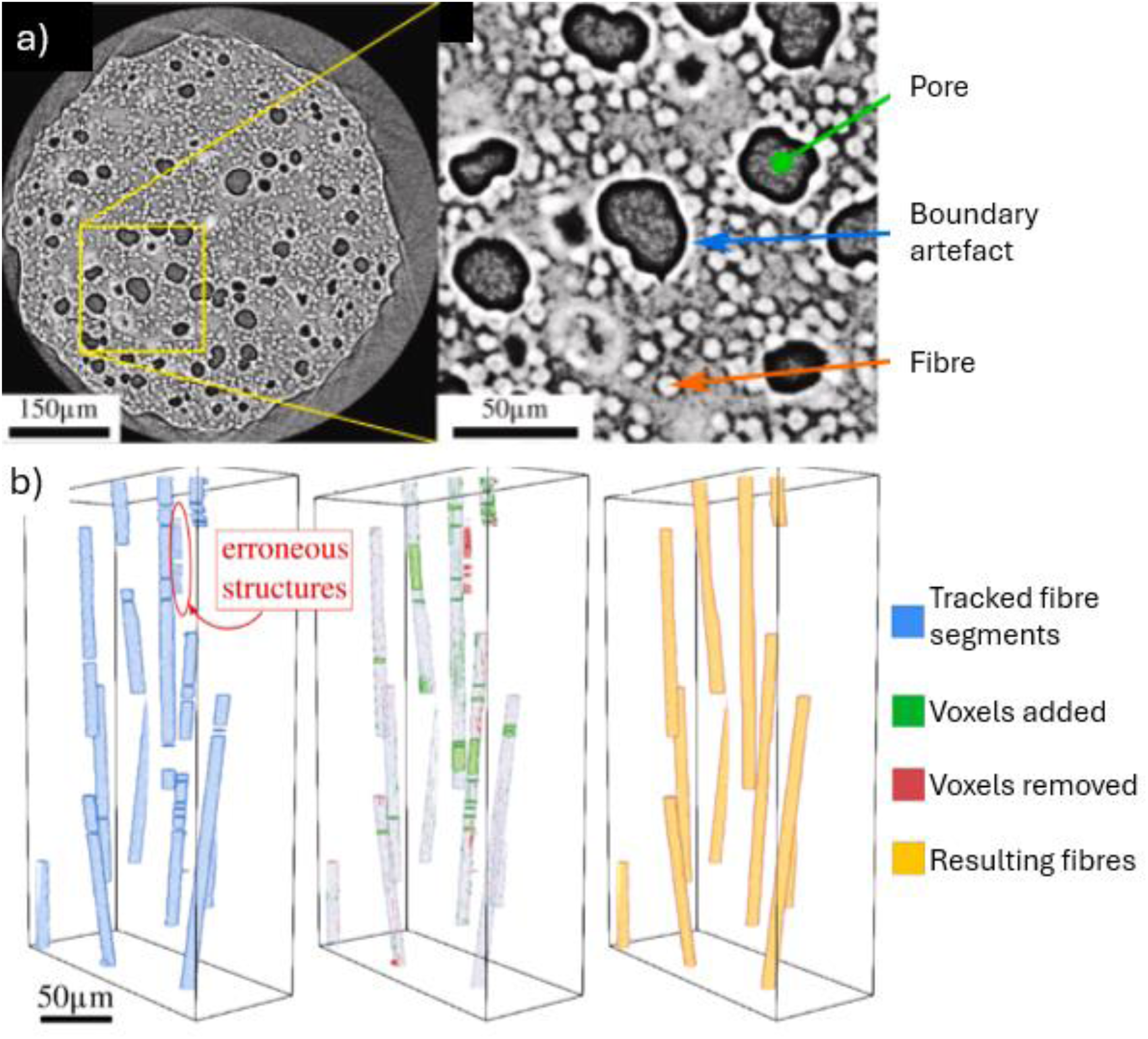
(a) sample 2D slice of tomographic scan of a PEEK 40 wt.% CF filament (after histogram equalisation), and (b) post-processing showing (left) fibre segments from the fibre tracking analysis, (centre)) morphological closing to add missing (green) segments and to remove a few erroneous (red) features and (right) the resulting fibre volumes. 42
Turning phases into finite element meshes
Meshing workflow
Discretisation for a geometry is closely linked to the numerical solver employed in the workflow. For instance, Finite Element (FEM) and Finite Volume Method (FVM) solvers, which are among the most widely used numerical methods in the engineering community, require a discretisation with nodes and elements (sub-domains formed by interconnected nodes). Other solvers, such as FFT-based and Finite Difference Method solvers, only require a regular grid. For such cases, image discretisation can be performed at either the initial resolution or after down-sampling (i.e., reducing the resolution by grouping pixels or voxels), which significantly simplifies the meshing process. Meshless solvers, such as the Discrete Element Method, Smoothed Particle Hydrodynamics and peridynamics are available in the computational mechanics community, but applications in image-based simulation are not yet popular, possibly due to their limitation in accuracy of stress/strain predictions and the lack of standard software packages. Producing high quality FEM meshes of the complex 3D geometries typical of textile composites remains a challenge, as discussed elsewhere. 89 FE meshes for composites are generally classified into two categories: conformal and non-conformal (voxel) meshes. The difference between these two types of meshes lies in how they represent the boundaries between the phases as illustrated in Figure 9. Obtaining a conformal mesh is typically more desirable, but more difficult, than generating a voxel mesh.
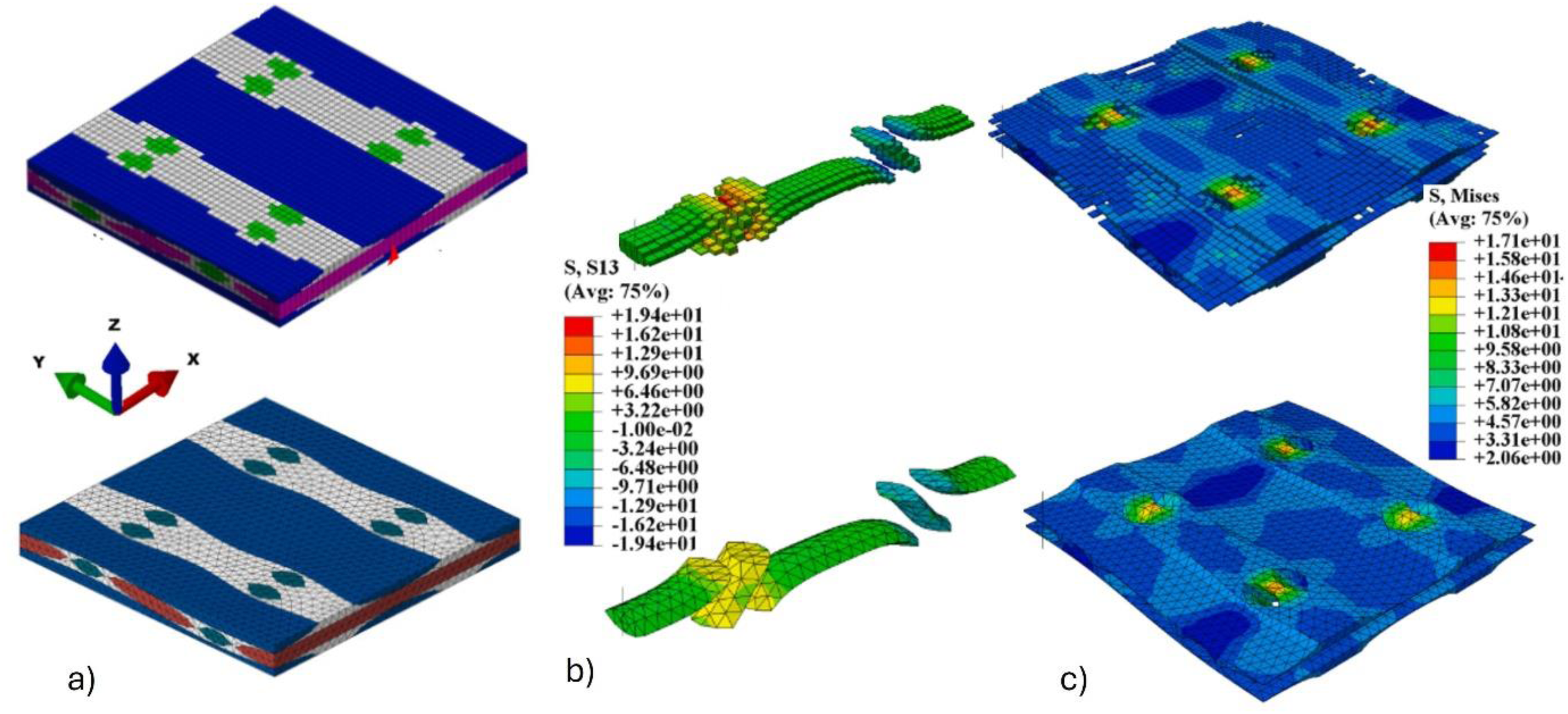
Voxel (top) and conformal (bottom) RVE representations of a 3D woven composite subjected to warp tensile loading showing (a) the meshes, (b) shear stress in one of the binder yarns, (c) comparison of von Mises stress fields. 90
The nature of X-CT images lends them to
The generation of a conformal mesh begins with post-processing of a segmented X-CT image. Initially, surfaces of the phases need to be generated. This can be done by extracting interfaces directly from a voxel mesh of the segmented X-CT image and applying an explicit smoothing algorithm e.g., Laplacian smoothing94,96 directly on these surfaces or those constructed using marching cubes algorithm from the voxel mesh. 97 Alternatively, implicit surfaces may be constructed by defining a signed distance function for each phase (e.g., fibres or yarns) and employing a level-set method to determine their boundaries. The resulting boundaries then can be smoothed using Gaussian filter (“blur”) to remove irregularities that Laplacian smoothing is unable to eliminate. 67
Once the surface meshes have been obtained, it is possible to generate a volume mesh. Typically, a tetrahedral volume mesh would be created for composites and a mesh consisting of hexagonal or triangular prismatic elements would be generated for models of dry fibre reinforcements 98 or laminates.66,81,82 An example of a conformal mesh of a textile composite is shown in Figure 9. This example illustrates a mesh that is generated by applying an explicit smoothing to a voxel mesh to obtain surface meshes of the yarns. The surface mesh is then remeshed to improve their quality and the resulting surface meshes are used to generate a tetrahedral volume mesh. In some cases, for example when a macro-scale model of a composite is required, a generation of the mesh can be relatively simple. Seon et al. 99 generated a hexahedral mesh of a composite laminate with local waviness by morphing a rectangular grid mesh to fit segmented X-CT data.
Challenges when generating meshes for composites
Some of the challenges in generating conformal meshes relate to general difficulties of meshing finite element models containing small features such as sliver-like regions between yarns, which require excessively small element size near these features. A common approach to address this issue is to increase the size of the problematic regions to allow for larger element size. In the case of textile composites, this would typically mean introduction of an artificial gap between yarns, which is made feasible by the implicit description of the geometry. However, these adjustments need to ensure that the overall and local fibre volume fractions remain realistic.
Another common difficulty when using X-CT images to build a model of a composite is the question of selecting an RVE of an appropriate size. For numerical simulations at the micro- and meso-scales, it is often desirable to prescribe periodic boundary conditions (PBCs) on the edges of the RVE because PBCs require smaller RVEs to be statistically representative of the homogenised properties.37,95,100 However, the 2D and 3D images used for image-based modelling are unlikely to have an inherently periodic structure. Some solutions have been developed for this problem such as modifying the geometry of the model to enforce periodicity at micro- 101 or meso-scales, 102 or using modified periodic boundary conditions, such as weakly periodic boundary conditions. 103 In all cases, it is important to remain vigilant because the boundary may not be sufficiently representative of the real microstructures.
Constitutive equations
Mechanical models for elements and interfaces
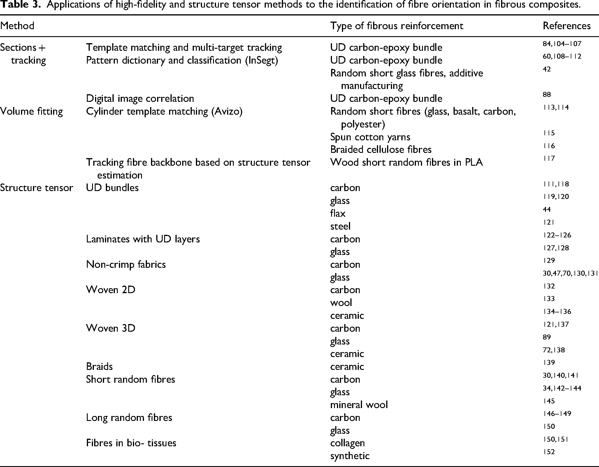
Once segmented into the constituent regions, the properties representative of each region and their interfaces to other regions must be applied. This can be for specific phases (e.g., matrix, reinforcement, interfaces), but also to ‘composite’ domains (e.g., yarn, laminae). The former is relatively straightforward; in the latter cases the properties can be determined from a smaller (image-based) sub-model or inferred from a knowledge of the fibre orientation. The orientation of fibres and hence the mechanical properties to be assigned to each finite element can be obtained directly from X-CT if the individual fibres have been tracked (see sub-section: Segmenting images into distinct phases and Table 3). In other cases, the average fibre orientation within each element can be determined by SAXS tomography (sub-section:Small-angle scattering tensor tomography, or by structure tensor analysis from X-CT images even when the contrast or resolution is not sufficient for the individual fibres to be segmented (see Table 3).
Applications of high-fidelity and structure tensor methods to the identification of fibre orientation in fibrous composites.
Structure tensor analysis47,130,142 allows local fibre orientations to be estimated without tracking individual fibres. In the structure tensor method, the principal direction and the degree of microstructural anisotropy can be calculated from the structure tensor 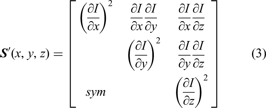
Structure tensor analysis can be undertaken using open-source or commercial software (see Table 1). Using this approach, the degree of local fibre orientation distribution can be inferred for each volume element in a finite element model and the relevant mechanical property tensor assigned.
Once the parameters of the fibrous material in the elements are identified, the anisotropic stiffness matrix is calculated using micro-mechanical theories,153–155 and then the homogenised stiffness matrix of the material is calculated. This is performed either using analytical homogenisation methods, such as orientation averaging or Mori-Tanaka, 156 or with FE homogenisation, which involves the solution of six boundary value problems, corresponding to different elementary loading patterns. 157 When assigning the properties to a yarn in a woven or braided material, it is important that the properties are aligned with the fibre orientation direction at each location rather than the overall coordinate directions (e.g., the warp or weft directions).
Image-based models play an important role in modelling inelastic behaviours. For example, the resin matrix of polymer matrix composites (PMCs) is typically modelled with an isotropic elasto-plasticity constitutive law. 158 As a consequence, the behaviour of lamina or fibre yarns at the mesoscale is often described with elastic-plastic models, though anisotropy is required due to fibre orientations. Several studies have demonstrated that incorporating plastic behaviour is crucial for the model to accurately reproduce experimental measurements (see. e.g.,159,160).
Damage initiation and propagation criteria
There is a plethora of mechanisms by which damage can occur in composite systems (See Figure 10) and these include:
Sequence of microscale damage and crack propagation for a ply of a double notched (−45°/90°/+45°/0°/−45°/90°/+45°/0°)s carbon fibre epoxy composite sample under progressively increasing tension along the fibre-axis (z) using a phase-field regularised cohesive zone model (PF-CZM) with softening laws. 161
One approach is not to model such microscale damage explicitly (with its heavy computational cost) but to use a continuum damage mechanics (CDM) approach 163 within a FE framework. Here, the accumulation of microscopic damage such as matrix cracks, fibre breakage, and delamination at finer scales can be accounted for indirectly treating the material as a homogeneous continuum instead, allowing for analysis of the overall structural response as damage evolves throughout the material. In certain cases, microscale image-based modelling can be used to develop CDMs at a coarser length scale. CDM requires two material models: one for damage initiation and one for damage evolution. It uses damage parameters to describe the damage in composite constituents which start at zero (no damage) and progress to one (completely damaged). These increase gradually such that damage can progress within an element as well as throughout the mesh. Separate damage initiation criteria can be used to describe matrix, fibre, interfacial and intralaminar failure. The degradation in the mechanical response can be gradual as the damage variable increases or represented by a step-jump. Beyond quasi-static material models, dynamic behaviour, such as impact 164 and fatigue 165 have also been modelled for fibre reinforced composites. However, image-based modelling of these dynamic behaviours is in its infancy. It is anticipated that this will increase as more experimental data from X-CT observations become available.
Crack propagation modelling can be broadly divided into two different strategies: sharp interface and diffuse interface approaches where the crack is smeared over a small but finite length. In the FE modelling, the fracture process is typically modelled across the three constituent phases (fibres, matrix and interfaces) using pre-inserted cohesive interface elements. This has the drawback that it is possible that the locations of the cracking mechanisms are not quite right, which may affect the micro-damage processes and their responses on the global scale model, although adaptive meshing can be used to vary the crack path. 166 Crack growth is allowed to progress through each of the three phases without restriction. Matrix cracking and interfacial debonding behaviour can most simply be modelled by the breaking of cohesive elements using one of two criteria, namely a maximum stress failure criterion, which is based on the highest ratio of the stress to the peak stress in each of the three orthogonal material directions, or a quadratic criterion, which is based on a quadratic combination of all three ratios, with the latter criterion being particularly useful in modelling mixed-mode behaviours. 161
Much less commonly, meshless methods have been applied. They avoid a predefined fixed connectivity between the nodal points used to define the geometry. As a result of the connection-free nature of the nodal discretisation, any crack propagation paths can be efficiently embedded geometrically within the numerical model. Often, they are used in conjunction with CDM to model damage evolution and crack propagation. Despite the higher accuracy and flexibility, meshless methods tend to be more difficult to master. Of these methods, the extension of FEM into XFEM is gaining traction. 167 It retains some advantages of the FEM but allows the singular stress state at a crack tip to be reproduced while allowing multiple cracks or arbitrary crack propagation paths to be simulated on an independent unaltered mesh. Critically the mesh does not need to conform to the virtual crack path.
Modelling/simulation
Here we consider IBM at specific scales (sub-section:Modelling at specific scales ) before looking at multiscale modelling (sub-section: Multiscale modelling). Figure 11 summarises the way information flows between these scales. It is worth noting that the output from microscale modelling can be used to develop the constitutive relations for yarns/tows for those composites having mesoscale features, such as 2D woven composite materials. Theseoutputs can also be directly used as inputs for macroscopic modelling of composites without mesoscale features, such as unidirectional composites. In this respect, the key issues limiting the application of IBM are chiefly image resolution and segmentation. Resolution is a double-edged sword, in that for IBM, higher resolution imaging is not necessarily better; rather, it depends on the specific scale of the analysis and objectives. For high-resolution images, extensive microscale surface waviness can trouble FE mesh quality, as well as giving difficulties in segmenting individual fibres in microscale models.
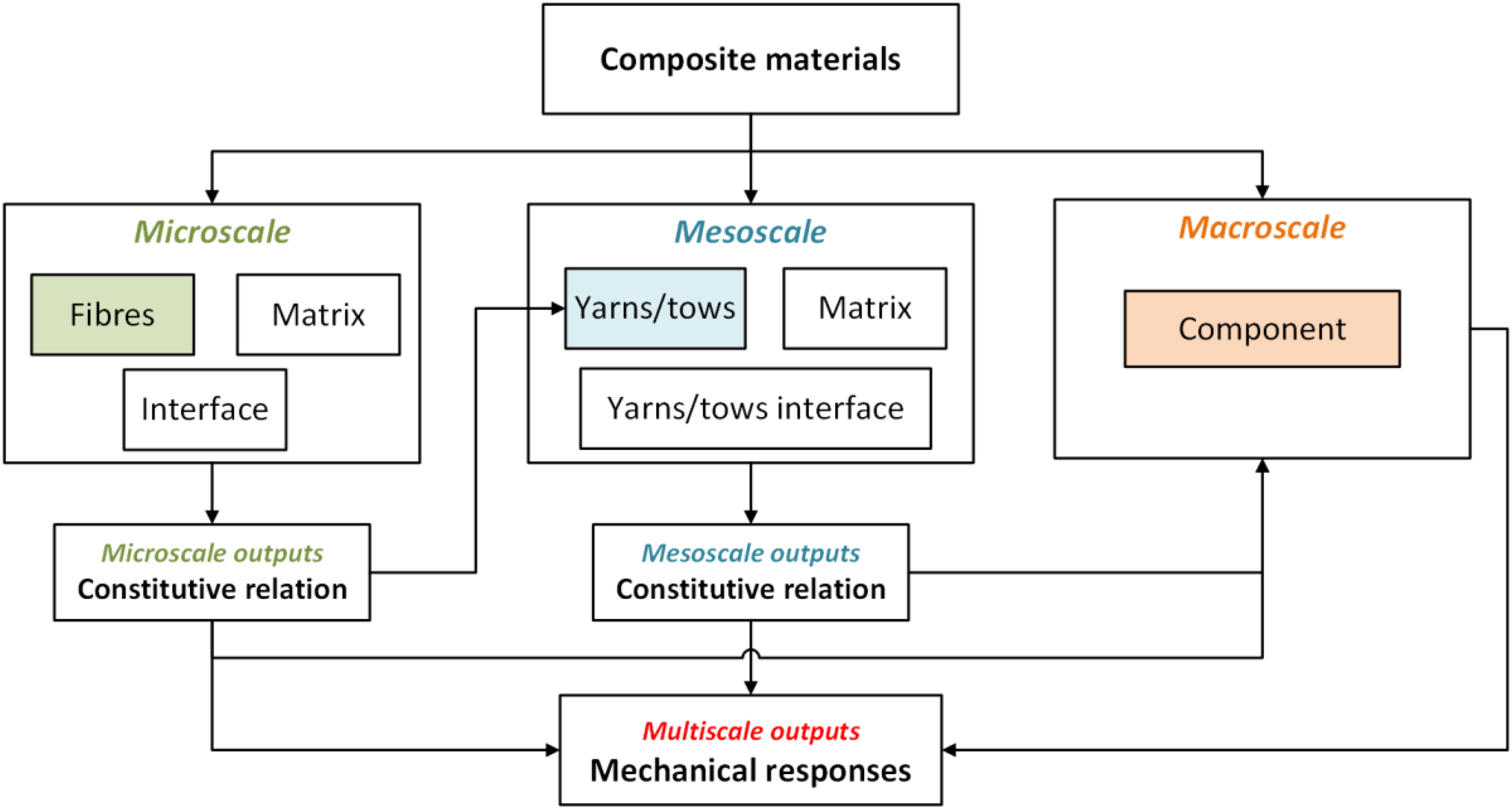
Strategies for composite modelling at different scales.
Modelling at specific scales
Modelling interfacial debonding through cohesive surfaces or elements requires that the segmentation process creates surfaces which are ideally relatively smooth. Sub-section: Segmenting images into distinct phases has identified strategies that can help to achieve this. Fibres may be straight at the scale considered, but segmentation errors often lead to slight misalignments or waviness due to noise. These errors can be critical in predicting some microstructurally sensitive properties, such as compressive strength. Meshing is often difficult when fibres are very close to each other, leading to poor mesh quality and convergence issues due to distortions. Nevertheless, these high local fibre volume fraction regions are crucial in predicting damage development, failure and permeability.
170
The embedded elements method may help resolve meshing issues, but it does create volume redundancy concerns and the combination with cohesive zone modelling (CZM) is not straightforward.171,172 Microscale models also need accurate information on the fibre orientation,
168
meaning that simply meshing segmented images is insufficient. Often this is needed at the individual fibre scale rather than the fibre bundle scale which means that high-fidelity methods can be more appropriate than structure tensor methods (see Table 3).
Surface imperfections, such as pits or bumps extending over tens of micrometres, impose constraints on FEM by limiting the element size. This significantly increases computational demands and complicates numerical damage simulation. High-resolution imaging, typically achieved through lab-based X-CT at 4–8 μm resolution,
21
can provide detailed and accurate information about surface flatness, which may include many surface imperfections at the micrometre level. Material defects, such as porosity and cracks, will often need to be considered in macroscale image-based modelling. Typically, most synchrotron scanners have fields of view at the centimetre scale, although a notable exception is the BM18 beamline at the European Synchrotron Radiation Facility. Consequently, whole component scanning is usually undertaken using lab X-CT scanners. Many composite components are essentially flat panels which are not easy to scan in conventional scanners. In some cases, laminography
174
can be used to overcome this issue. If the lower-scale model is RVE-based, then it can be difficult to pass on damage-related information because most homogenisation methods often focus on the elastic properties. This inherently limits the accuracy of macroscale models. This issue and potential solutions are discussed in more detail in sub-section: Multiscale modelling.
Multiscale modelling
Although image-based methods are often appropriate at specific scales (micro, meso, macro), one often needs to link the image-based and continuum-based models in a multiscale manner, where the effective behaviour of the upper scale is derived from averaging the behaviour at lower scales. Numerical homogenisation is a well-established technique for composites, 175 at least when the length scales are well separated, and one can determine a periodic RVE. A clear separation of scales between the meso- and the macroscales can break down where the size of the heterogeneities at the mesoscale is comparable to that of the sample. Also, determining a proper RVE37,176 for complex composite structures 177 can be challenging as the underlying microstructure changes continuously within the specimen. This difficulty is exacerbated in image-based approaches that account for both geometric178–181 and material variabilities,182–184 resulting in fully stochastic models. Direct simulation of large-scale specimens, while resolving all the microstructural details demands the use of high-performance parallel computing and dedicated domain decomposition methods185,186 with specialised preconditioning techniques.187,188
Alternative, more computationally efficient, strategies have been proposed by constructing an approximate heterogeneous macroscale model where the underlying microstructure is not fully resolved, but is still taken into account. One may, for example, filter the underlying (micro-/meso-scale) heterogeneities, 189 or perform only local homogenisation to determine varying apparent properties138,190–194 at a scale compatible with the computation at hand. These approaches could be extended into the framework of multiscale FEM195,196 by projecting or condensing concurrent solutions at a lower scale onto the computational mesh.197,198 Finally, global-local approaches 199 allow the coupling effort to focus only on regions of interest where a fine description of the lower scale is required. However, ensuring the continuity between the local and global models, especially when strong heterogeneity crosses the interface, remains a significant challenge.200,201
Surrogate modelling202,203 serves as a mathematical approximation technique that replaces high-fidelity simulations or experiments by learning the input-output relationships from existing data. It is widely used to accelerate complex analysis and optimization tasks by significantly reducing computational cost while maintaining acceptable predictive accuracy. This is particularly important in progressive damage simulations, where finite element (FE) analyses involve severe geometric and material nonlinearities and demand intensive computational resources. Various surrogate modelling strategies have been developed to suit different simulation scales, each with distinct assumptions and trade-offs. Among the most widely adopted approaches are Gaussian Process Regression (GPR), Reduced-Order Modelling (ROM), and Artificial Neural Networks (ANNs). GPR is a kernel-based Bayesian regression technique that offers high predictive accuracy along with uncertainty quantification, making it especially effective in small-data scenarios - though it comes with considerable computational expense. 204 ROM reduces the dimensionality of high-fidelity models by projecting them onto a low-dimensional subspace, enabling fast predictions at the cost of reduced accuracy in highly nonlinear regimes. 205 ANNs, loosely inspired by the architecture of the human brain, are capable of capturing complex nonlinear patterns from large datasets, but they often require extensive training data and suffer from limited interpretability.202,206–208
Given the varying requirements across scales, surrogate modelling approaches should be tailored accordingly. At the microscale, where capturing fine-grained nonlinear behaviour is essential, high-accuracy methods such as GPR are typically preferred. At the mesoscale, a balance between accuracy and computational efficiency is often sought, making both GPR and ANNs viable options. At the macroscale, the focus shifts primarily to computational speed, favouring surrogate strategies like ROM and ANNs. Despite their growing adoption, surrogate models still face several challenges, most notably the lack of integrated multiscale surrogate frameworks that can seamlessly bridge different physical scales within a unified modelling architecture. However, the developing ANNs, which demonstrate superior cross-scale modelling capabilities, offer valuable insights into the development of multiscale surrogate modelling strategies. For example, Kim et al. 208 developed a deep learning driven surrogate model for a nanocomposite (see Figure 12) to investigate its inelastic behaviour of microstructure. The surrogate model was able to mimic both the macroscopic stress strain response and the microscopic strain field with a dramatic decrease in computation time.
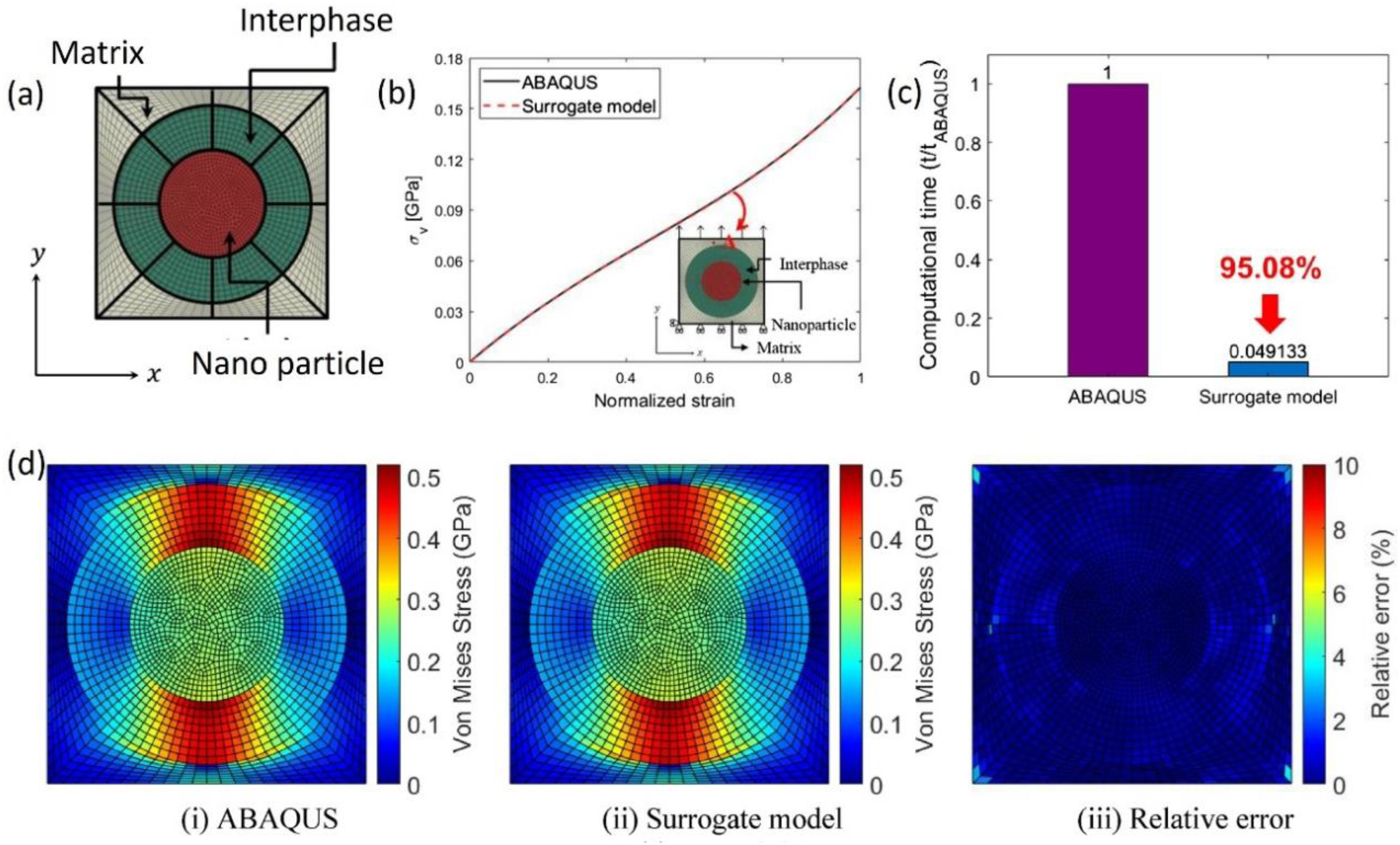
Surrogate modelling of nanocomposites. (a) unit cell for the nanocomposite (FE model), (b) macroscopic stress-strain response and (d) microscopic stress field comparison of the surrogate and FE models, comparison of (c) the computational time and (d) the von Mises stress fields associated with the surrogate and FE models. 208
Applications
It is not possible in this review to cover all the applications of image-based modelling undertaken so far; rather the following sections are illustrative of the applications that can be served by such approaches and the aspects that need to be considered when doing so. Many of the examples are taken from the polymer composites area, but the approaches can easily be applied to other composite systems.
Composite manufacturing
Many polymer, metal and even ceramic matrix composites are formed by infiltrating the dispersed reinforcement (often in the form of a textile or fibre preform) with a fluid (e.g., liquid resin, slurry or molten metal). In all cases, the aim is to produce a fully dense composite in the shortest possible time. In the case of metal matrix composites, the temperature and time at temperature are often minimised to prevent interfacial reaction. In polymer infiltration pyrolysis (PIP) of ceramic matrix composites, the number of infiltration steps is of concern, while in polymer infiltration of polymer matrix composites, air entrapment and fibre-free/resin-rich areas are of interest. As a result, X-ray imaging is being increasingly used to study the infiltration processes aided by simulations used to design and optimise the infiltration processes. 209
Changes in the reinforcement distribution can occur during processing, either compacting and thereby closing pore channels, or separating them to create reinforcement-free regions. 210 To capture this, Yousaf et al. 46 have used the digital element approach 211 to model how nesting and compaction of carbon fibre textiles can reduce the pore spaces and, thereby, the changes in permeability as the pore channels close with increasing pressure. 45 In other cases, textile reinforcements (dry or prepreg) are deliberately deformed into a desired 3D shape (i.e., draped) onto a mould. In such cases, X-CT can be used to help develop mesoscale simulations that incorporate the typical modes of textile deformation – shear, biaxial tension, and compaction. 212
With regard to liquid composite moulding processes, a great deal of work has been undertaken using image-based modelling to predict the permeability of fibrous networks. These approaches have considered both the mesoscopic pore channels between tows and the microscopic channels within them. In this respect, a round-robin study (international Virtual Permeability Benchmark) 170 has evaluated the state-of-the-art of existing numerical approaches for microscale permeability prediction by considering a single fibre bundle region of interest (400 fibres wide and having a length of ∼500 µm) that had been extracted from an X-CT scan of a twill-weave fibre glass-reinforced composite. The round-robin study concluded that the predictions of axial permeability showed less scatter (presumably because of the simpler flow paths) than the transverse permeability and also that for microstructures with unknown principal directions, or with anisotropic effects, applying symmetric or no-slip boundary conditions was not appropriate and a method that determines the full permeability tensor is needed. The permeability of such microstructurally realistic models can then be used as an input for mesoscale calculations of flow through the fabric to deduce its macroscopic permeability. This was the topic of the second phase of this round-robin on the image-based permeability prediction, 213 which highlighted the need to take great care in selecting an image with a mesostructurally representative RVE, which may or may not contain continuous inter-tow flow paths that dominate the intra-tow flow.
With regard to woven fibre composites, Ali et al. 56 found that for a 3D angle interlock carbon fibre composite the percentage of areal gaps in the warp direction were less than in the other two directions, but that these were reduced less than for the other two directions upon compaction. The flow channels for flow in the weft direction are shown in Figure 13(a). Similar approaches would also be appropriate for ceramic processing by PIP, where the situation is complicated by the fact that the channels reduce in size and connectivity each PIP cycle as full densification is approached.
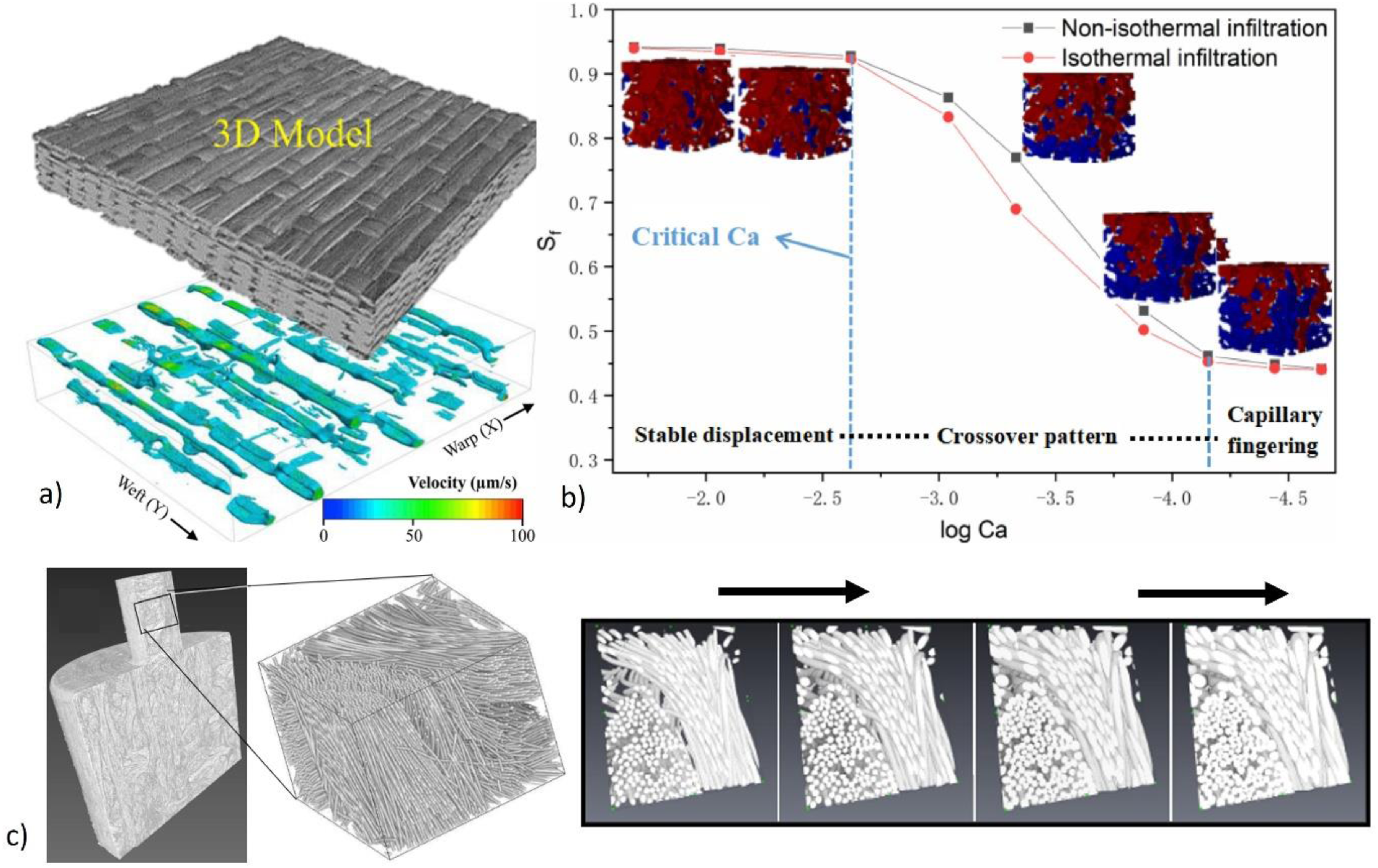
Examples of infiltration modelling. (a) X-CT image-based model for a 3D angle interlock carbon fibre fabric (top) and resin flow fields (bottom) showing flow paths in the weft direction, 56 (b) predicted flow of liquid Al metal through an IBM of porous SiC showing the steady-state fluid saturation, Sf, with respect to capillary number, Ca. The insets show the non-isothermal distribution of fluid (red) in the SiC (blue), 214 (c) time-lapse sequence showing a micro-scale pore chemical vapour infiltration simulation based on a 3D image of a C-fibre preform from an X-CT scan (left). 215
Image-based infiltration studies have also been undertaken for particulate composites. For example, Guo et al. 214 used a pore-scale, non-isothermal two-phase flow numerical model to describe the infiltration of liquid Al metal into a SiC porous preform. They found that the infiltration pattern transitions from stable displacement to capillary fingering due to changes in the local meniscus dynamics, and that void trapping stability is higher in the capillary fingering pattern (see Figure 13(b)). As a result, there is a critical capillary number (Ca) value, above which the local macroscopic void concentration can be avoided.
CMCs such a C/C composites are often produced by chemical vapour infiltration (CVI) involving the infiltration of a heated fibrous preform by the chemical cracking of a vapour precursor. The density of materials prepared by CVI relies on processing conditions and the microstructure of the preform. Similar image-based methods to those described above can be used, but with gas transport modelled rather than liquid transport. In Figure 13(c), a random-walk-based infiltration framework has been applied for the fibre-scale modelling of chemical vapour infiltration of a carbon fibre preform.215,216
Elastic properties
One of the primary applications of image-based modelling in composite materials is predicting elastic properties. Studies leveraging advanced imaging techniques, such as micro-CT and X-ray scattering tensor tomography,30–35 have enabled researchers to extract detailed information about the effect of fibre orientations, volume fractions, and local microstructures of composites, which can both elucidate the knock-down associated with imperfect fibre/yarn alignment and manufacturing defects, as well as point the way to improved composite designs. Overall, the feasibility and quality of IBM depends on two main factors: a) image quality and resolution; and b) image recognition, which involves extracting modelling information from the image, such as image segmentation and image structure tensor computation. As regards image quality and resolution, a detailed discussion can be found in section: Capturing image data. It is noteworthy that small-angle X-ray scattering (SAXS) tensor tomography (see sub-section: Small-angle scattering tensor tomography) can provide precise tensile modulus predictions for voxel sizes up to fifteen times larger than the fibre diameter. 30
Since, image recognition is strongly correlated with the type of composite material studied, this section considers different types of composite materials in turn. For unidirectional composite laminates, the most straightforward image recognition approach is to identify individual fibres from the image, making the study of fibre misalignments/waviness highly intuitive and compelling, including fibre centre line identification217,218 and machine learning (ML).
219
Structure tensor methods (see section: Constitutive equations)
121
are a good choice to process the images when their resolution is limited. There are two methods used in conjunction with the structure tensor method to enable IBM stiffness prediction. The first are
With regard to woven and braided composites, IBM studies are not as extensive as those on unidirectional composite laminates. Such studies have been hampered by the lack of suitable data segmentation methods. In this respect woven composites are easier to segment than braided composites because the yarn angle differences in woven composites are more pronounced (usually 0/90°), making the yarns (including warp and weft) easier to identify, enabling structure tensor and ML methods. For example, Liu et al. 89 employed voxel models (using structure tensors) derived from X-CT images to predict elastic properties. For braided composites, 220 segmentation can be difficult to accomplish as they exhibit strong periodicity in both the circumferential and axial directions and typically have small braiding angles. Consequently, reports to date have required lots of manual intervention. For example, Liu et al. 221 refined mesoscale models for five-directional braided composites, incorporating fabric compaction and yarn torsion to enhance the geometric model. However, recent progress on automated segmentation of 2D braided CFRP tubes using fibre-tracking methods (see section 3.1.5) is compared against an idealised textile model, which is formed by sweeping an ellipse, constrained to a fixed interface, along the mathematical path defined by the braiding process, in Figure 14. It is evident that the idealised model gives rise to a gap where the bundles cross, which decreases the stress distribution on the interface of cross-section area, compared to the IBM. While the predicted elastic properties are similar (Figure 14(c)) it is likely that this would lead to differences in the initiation of damage.
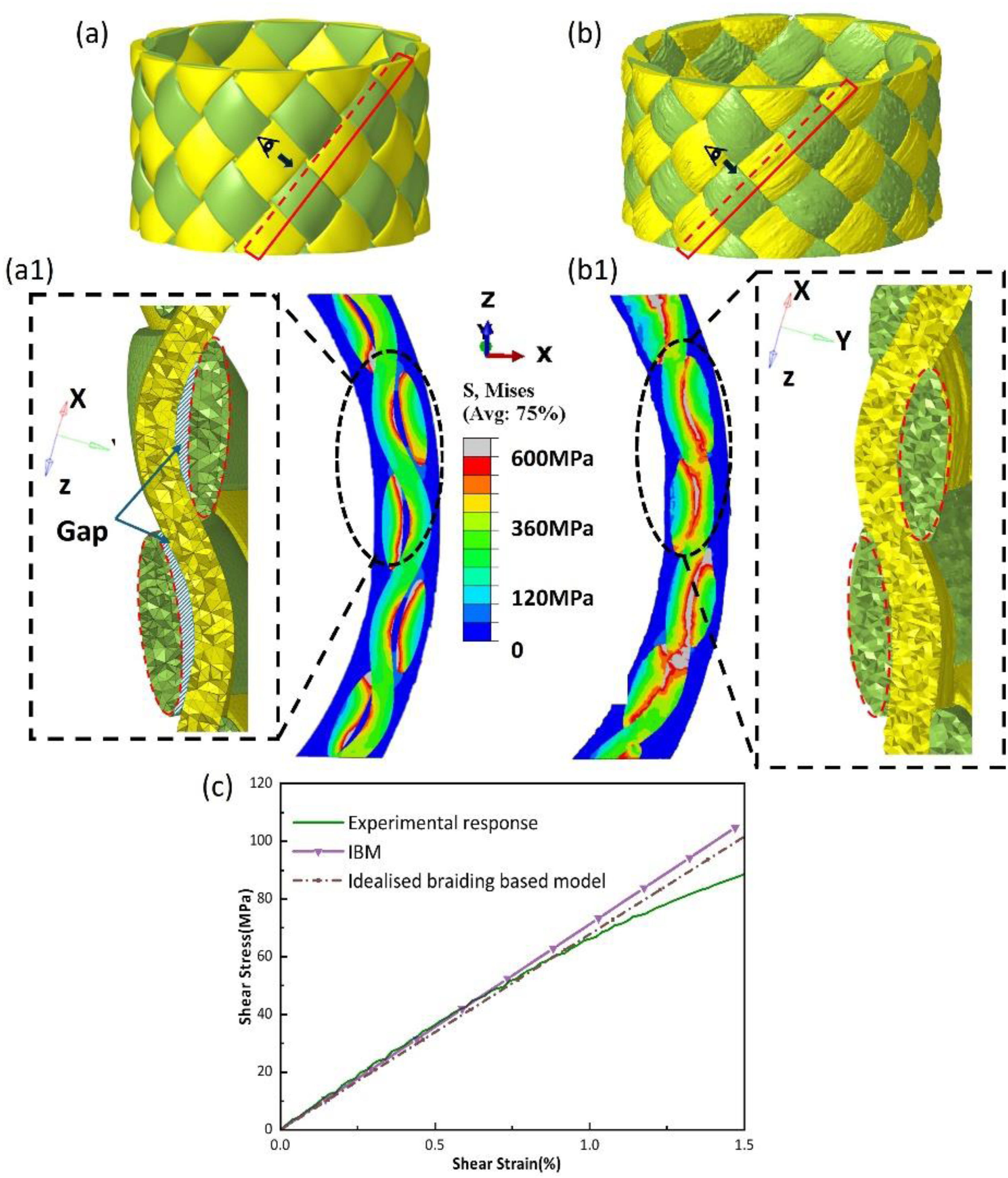
The comparison of the predictions of the elastic behaviour of an idealised textile model (a) and an X-CT derived IBM (b) of a braided composite. (a1) and (b1) show the braided bundle geometry (left) and the corresponding elastic torsional response (right) for the two cases, (c) displays the predicted elastic strain-stress responses alongside the experimentally measured response. (Courtesy He and Withers).
Thermal and transport properties
Given the importance of ceramic matrix composites (CMCs) and carbon-carbon (C/C) composites for high-temperature applications it is not surprising that much of the literature on IBM of these materials focuses on determining thermal properties, e.g., the linear thermo-elastic response135,222 or the thermal conductivity.223– 226 For example, researchers223,224 have determined the thermal conductivity of respectively 2D C/C and 2.5D CMC from image-based models which include material porosity. Lopez et al. 226 suggested a methodology using the advanced reduced-order modelling and machine learning to efficiently compute thermal properties on the images for a range of values of porosities and fibre distributions. Zahid et al. 225 accounted for an imperfect interface and contact conductance when IBM a 4D C/C, which led to more favourable results than idealised modelling 227 Foster et al. 136 used U-Net, a deep convolutional neural network implemented in Dragonfly, to separate the warp and weft tows of a compression-moulded silica phenolic composite comprising an 8-harness satin (8HS) silica fibre cloth. The local tow orientation vector, describing the longitudinal direction of the filaments in the fabric, was determined using the structure tensor analysis of the images. The in-plane conductivities were well matched, but the out of plane (OOP) conductivity derived from the image-based geometries showed a much more significant deviation from the analytical model when compared to the in-plane values. This is because the analytical model could only achieve the volume fractions observed in the X-CT images at undulation values that were much lower than the observed average undulation.
The mathematical similarity between heat conduction and mass diffusion has enabled similar approaches to be applied to other transport phenomena. For instance, Sinchuk et al.228,229 and Cao et al. 230 employed image-based models to assess moisture diffusion in PMC and to predict the resulting hygroscopic stresses, emphasizing the significant influence of porosity on these processes. Image-based models have also proven valuable in simulating the diffusion and reaction of oxidative species in self-healing CMCs103,231 demonstrating that the geometric variability inherent in real materials leads to non-uniform healing processes. Perrot 103 developed a 2D IBM method, enabling more accurate analysis of the self-healing processes considering oxygen diffusion, glass formation and flow dynamics, as illustrated in Figure 15. The results validated the effectiveness of the proposed method and display liquid (glassy) phase distribution, shown as Figure 15(c), which has a key influence on crack re-opening and healing process and further triggered further research on this topic, such as simulate material degradation to predict its service life.
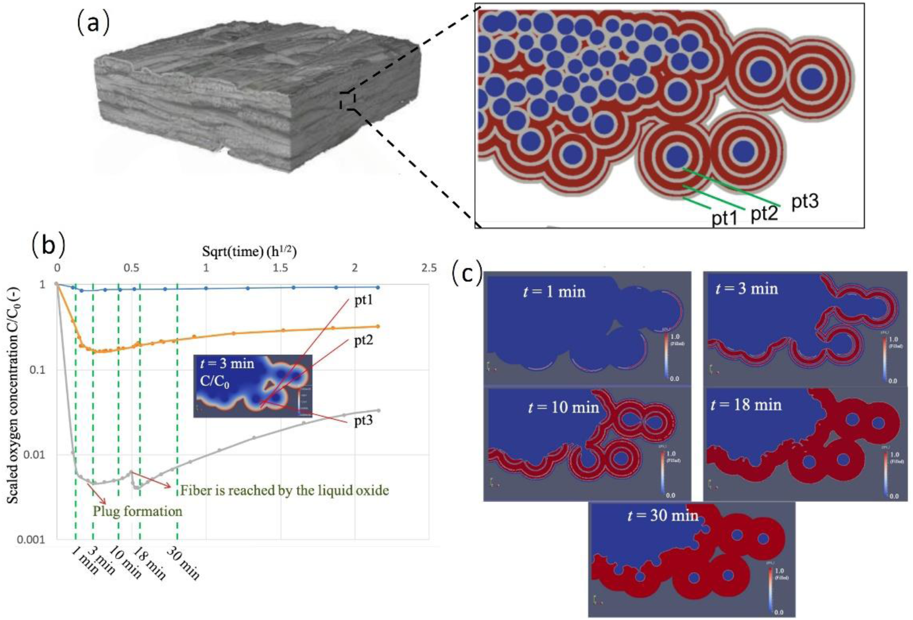
Modelling the oxidation of self-healing of SiC fibre ceramic-matrix composites (CMCs). (a) a mesoscale X-CT image (left), along with a magnified volume rendered image (right) showing fibres (rendered blue) and sealing matrix (red/grey). The evolution of the oxygen concentration at points pt1-3 is displayed in (b). (c) time-lapse sequence showing the predicted liquid (glassy) phase distribution from the IBM simulation. 103
These approaches can be readily extended to investigate other critical properties, such as thermal or electrical conductivity in fibrous systems, provided that the interfacial resistance is accurately captured.
Damage modelling
Understanding the sequence and importance of various damage mechanisms is critical for improving composite design for better efficiency and durability. Damage modelling reveals how pre-existing defects, interface strength and the composite constituents and architecture can influence the structural strength and failure processes. Damage modelling of composites spans microscale, mesoscale, and multiscale approaches, with each offering unique insights into failure mechanisms.
Regarding microscale IBM, the challenges and limitations have been discussed in sub-section: Modelling at specific scales. Generally, microscale IBM is a better candidate for numerically exploring the damage behaviour because it can take into account (a) defects, such as voids and fibre misalignment, and (b) the real distribution of the fibres, which can, for example, be far from ideal in natural fibre-reinforced composites. Iversen et al. 232 used fibre tracing to identify fibres of natural fibre composite and build the microscale FE model to simulate its damage behaviour, which validated that IBM is a reliable approach to include the non-uniform properties of fibres.233,234 Liu et al. 235 used fibre centre point tracking (see sub-section: Segmenting images into distinct phases; Fibre-tracking (tractography)) to distinguish fibres to build a 2D IBM model of UD composites to consider the influence of fibre arrangements and resin porosity on mechanical performance. The resulting IBM accorded well with the experiment results including the compressive modulus, strength and resin porosity which strongly influence the transverse compressive performance. Wan et al. 236 employed the structure tensor method to characterise the microscale fibre distribution and geometry within sheet moulding compounds (SMC). Based on this characterisation, two distinct models were developed to analyse the material's tensile response: (a) a model incorporating the actual fibre distribution, and (b) an equivalent homogenised model. The results indicate that the IBM model (a) yields a more accurate prediction of the tensile modulus. However, both models produce comparable results in terms of tensile strength, showing no significant discrepancy.
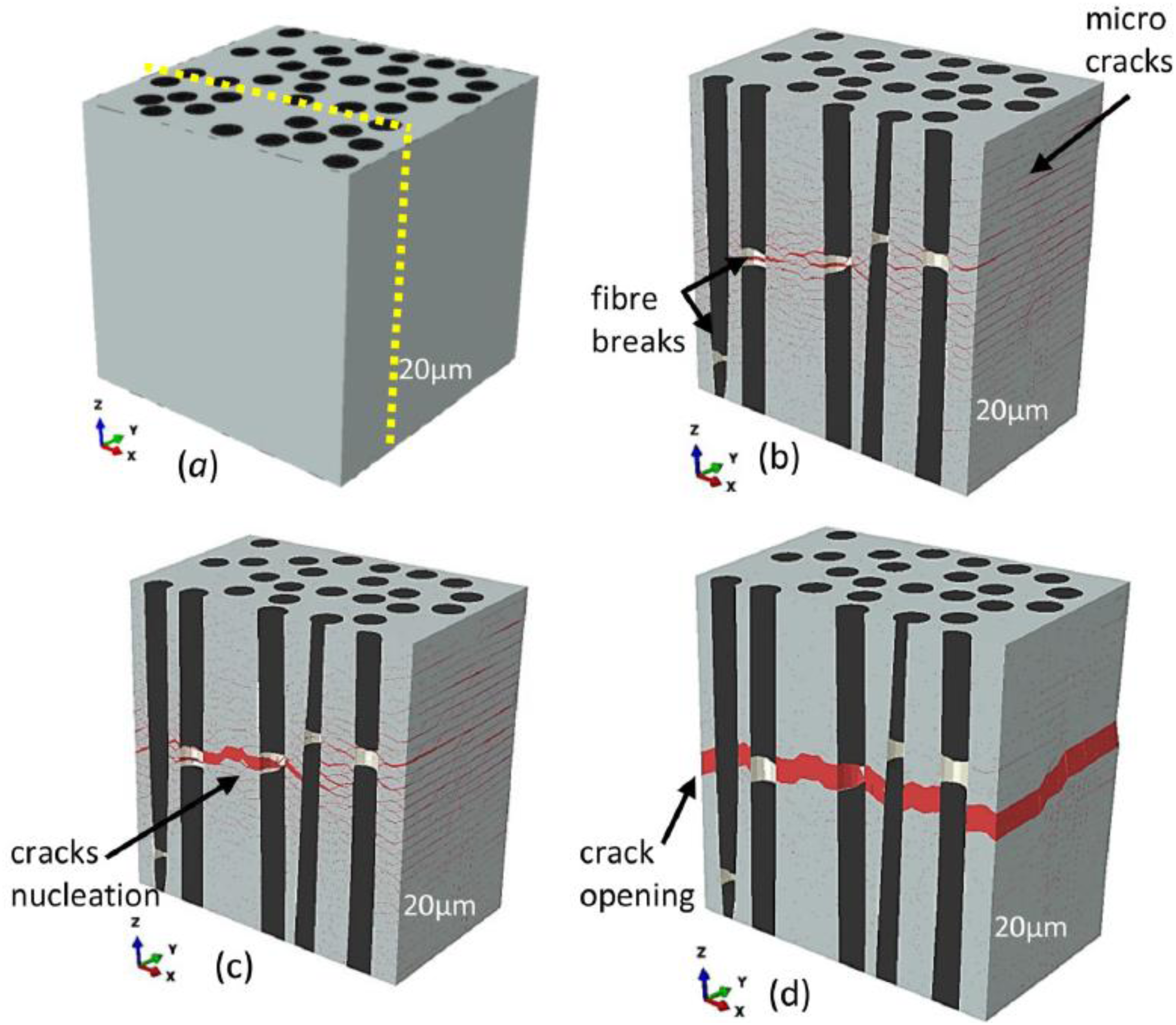
Mesoscale modelling generally relates to textile composites (2D and 3D woven, braided etc), whose mesoscale features (tows/yarns, matrix and interface) have a key influence on the structural strength and failure mechanisms. As mentioned in sub-section: Turning phases into finite element meshes, the main challenge is the segmentation of the yarns/tows. Liu et al. 89 developed an IBM framework for three-dimensional woven composites utilizing the structure tensor method, aiming to explore their damage behaviour under uniaxial tensile loading. The study revealed that while the elastic response of the material remains relatively insensitive to local variations in yarn geometry, these microstructural irregularities, such as yarn unevenness and defects, play a critical role in initiating and propagating damage, thereby significantly influencing the failure mechanisms. Similarly, Mazars et al. 191 developed an IBM approach, informed by in-situ tensile experiments on CMCs, to predict the onset of damage. By incorporating the actual fibre bundle geometry, the model accurately captured the maximum strain distribution in the elastic area and effectively identified the sites of damage initiation. Machine learning has also been used by Ai et al. for yarn identification for C/SiC composites tested under tension. 237 They found that the damage initiates from porosity (see Figure 16(b)) which then grows towards the interface between yarns and matrix and finally presents as macroscale cracks. This sequence shows a high degree of consistency with in-situ tensile images (see Figure 16(c)).
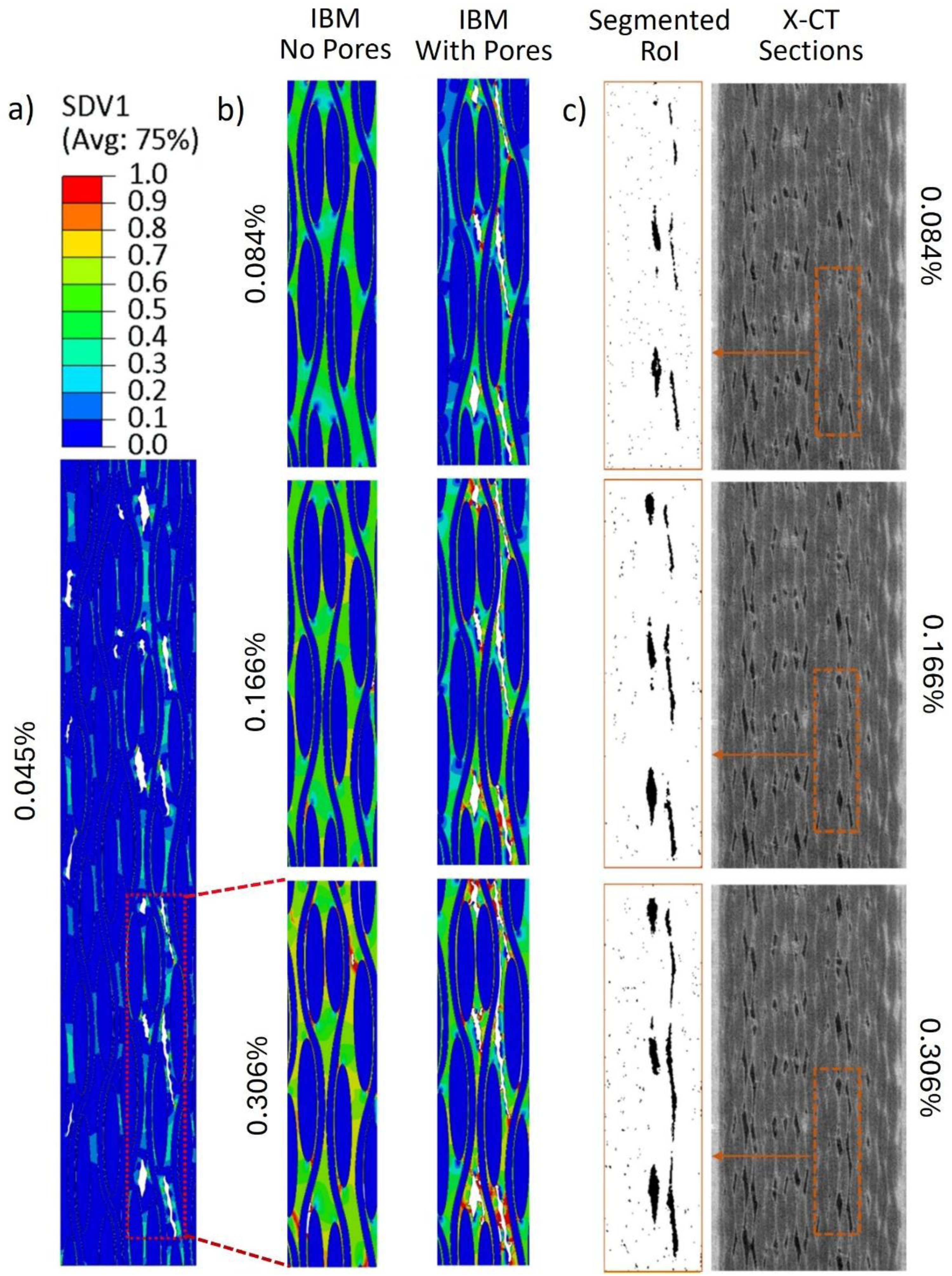
Evolution of damage (SDV1 = 0 to 1) for a CVI C/SiC woven composite. (a) the IBM at 0.045%, (b) regions of interest without (left) and with (right) initial porosity) and (c) in situ X-CT slices (right) and binarized damage (left) recorded at various longitudinal tensile strains after. 237
Peridynamics models are well suited to simulating fracture and damage problems. Wang et al. 238 used a peridynamics model (BB-PD) based on X-CT images of a C/SiC woven CMC segmented using a deep learning-based image recognition model to predict damage under increasing tension and the results are summarised in Figure 17. As loading progresses, damage appears where a significant number of peridynamic bonds between material points begin to fracture. This develops into a crack which extends from the surface into the interior. It is evident that damage primarily occurs at the interface between the fibres and the matrix, with minimal damage within the yarns. The image-based peridynamics model can accurately reconstruct the actual composite microstructure. It can effectively simulate various fracture phenomena such as interfacial debonding, crack propagation affected by defects, and damage to the matrix.
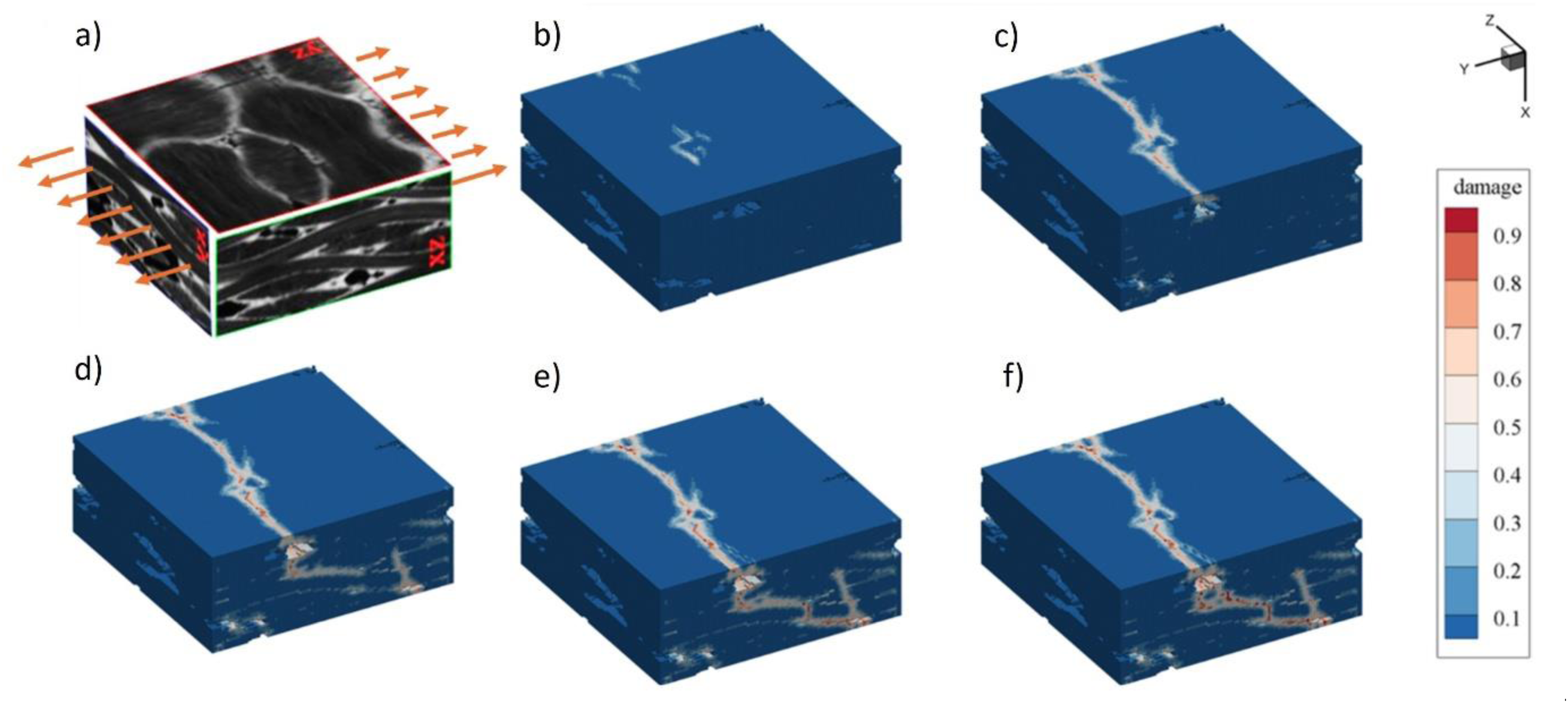
The 3D damage sequence for a woven C/SiC composite under a tensile load. (a) original X-CT image, (b) crack initiation, (c–e) crack growth, (f) failure stage. 238
With regard to particulate ‘composites’, image-based modelling is finding extensive application for the identification of cracking processes and the associated crack paths in concrete. For example, Ren et al. 239 created a two-dimensional meso-scale image based finite element concrete model from an X-CT scan simply by greyscale thresholding comprising aggregates (here rendered blue), cement paste (grey) and voids (white) see Figure 18. Cohesive elements with traction–separation laws were used to describe the cement paste and aggregate–cement interfaces. Under tensile loading a large number of images were simulated with statistical analysis demonstrating very different load-carrying capacities and crack patterns relating to the random distribution of phases. They found that the relative strength of cement pastes and interfaces dominates the microcracking behaviour (top), which in turn affects macrocracking (middle) and hence the load-carrying capacity. The strength was also inversely proportionate to the pore volume fraction. At a local level, the results show that a large number of interfacial microcracks initiate early on and gradually become stable before the peak load (point C) is reached. It can be seen that macrocracking is not evident at this point but as the displacement increases further, some aggregate–cement interfacial cracks continue to propagate and gradually coalesce with newly formed cracks to form macrocracks.
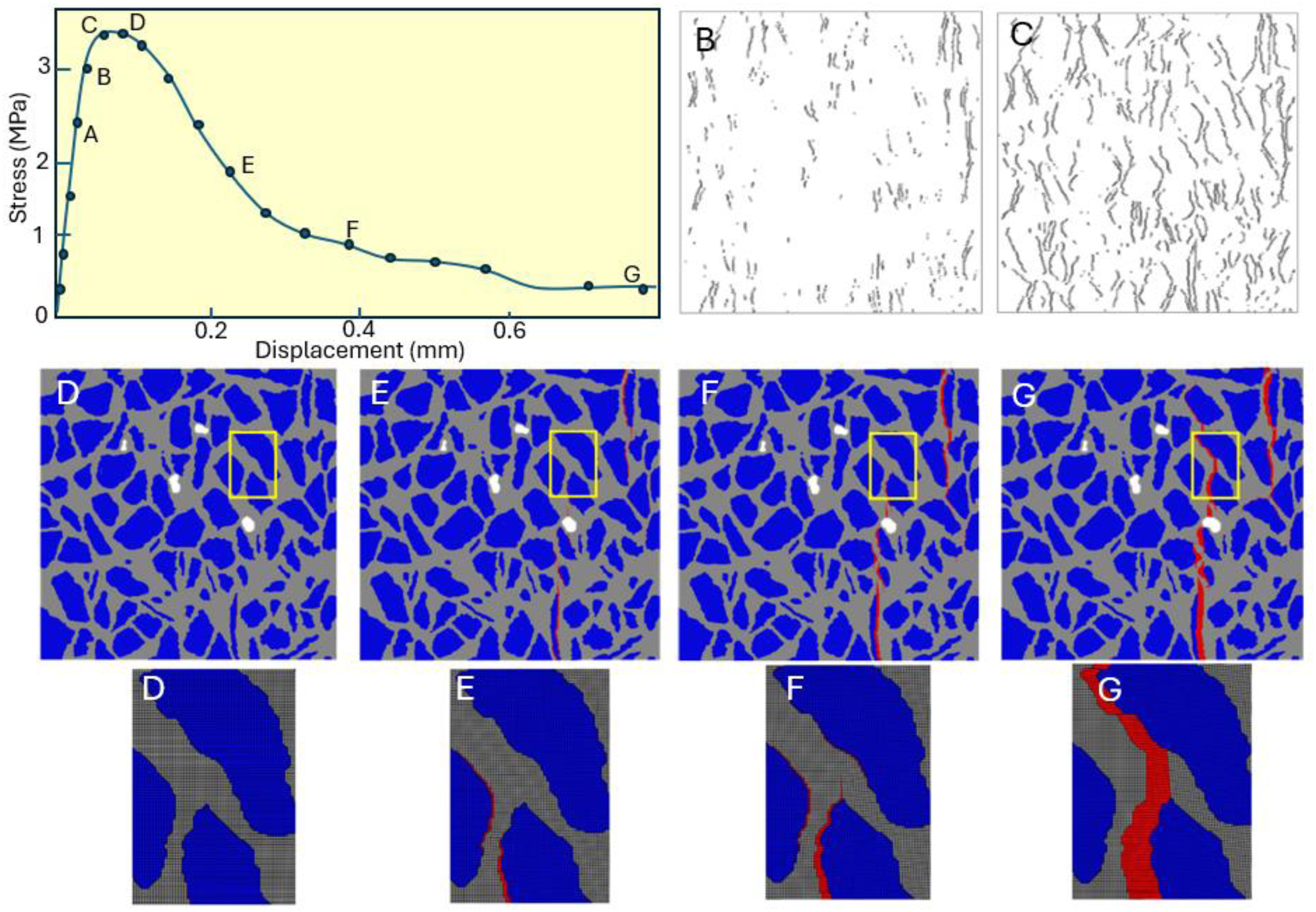
The evolution of pre-peak microcracking (top) and the associated macrocrack propagation (middle) and magnified region of interest (bottom) for a central cross section taken from an IBM under progressive tensile loading (horizontal axis) at the locations on the stress-displacement curve (top left) indicated by the letters. Paste is rendered grey, voids white, aggregate blue and the macrocrack red. The peak strength corresponds to stage C. 239
Validation with experimental results
Validation is a critical aspect of image-based modelling, ensuring that simulations reliably replicate real-world behaviour.
Since many IBM models are established on the basis of X-CT, it is perhaps not surprising that time-resolved X-CT imaging (often referred to as 4D X-CT (3D + t)) is frequently used to validate the predictions of the IBM.244–247 It can be coupled with additional post-processing techniques to validate the models, providing a better understanding of the effect of the microstructure on the behaviour of the composite, including the role of defects introduced during manufacturing and subsequent damage initiation.242,248–250 In this respect, many X-ray CT scanners can accommodate loading or environmental stages to reveal the damage initiation and propagation sequence under increasing loads, including tension, 246 compression, 83 torsion,247,248 bending, 245 and cyclic loading.251,252 The direct observation of the reconstructed volume can be used to qualitatively determine the damage scenarios, highlighting the influence of the mesostructure of the material (see for example for PMCs,248,253 CMCs,191,249,250,254 and for concrete 242 ) and as a means of verifying the veracity of the damage initiation criteria. A number of illustrative examples are shown in Figure 19 covering particulate, 2D cross-ply laminates and braided materials.
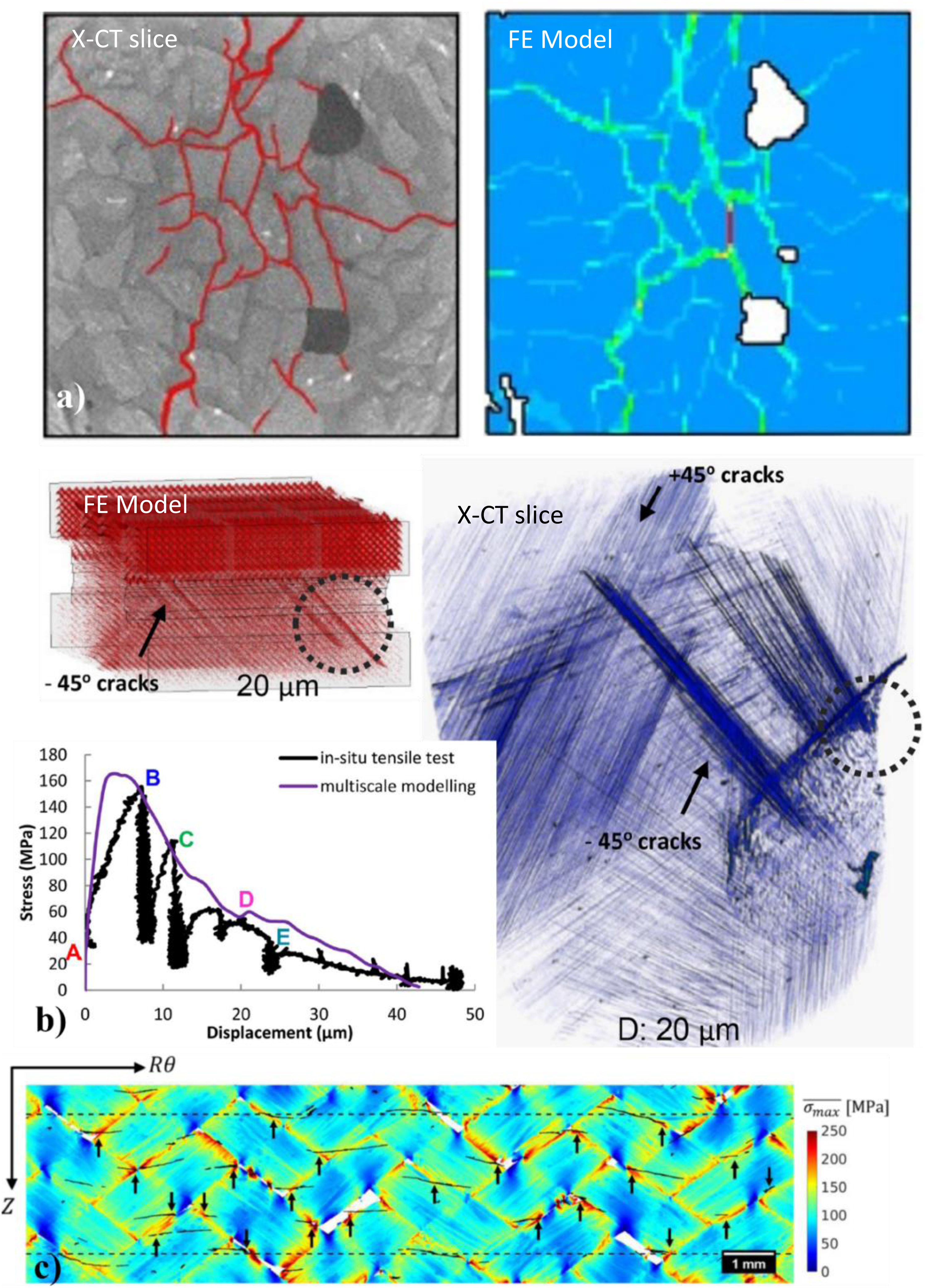
Comparison of image-based modelling with experiment. (a) Crack patterns on a longitudinal X-CT slice through a 40 mm concrete cube (left) under compression (vertical axis) and the predicted maximum principal strain contours for the IBM (right) 243 (b) measured and predicted stress-displacement curves for a FE multiscale IBM of a double notched cross-ply CFRP laminate tested in tension along with the predicted damage pattern (top) and the observed pattern (right), 161 (c) maximum principal stresses in the external sublayer (L4) of a braided SiC/SiC tube superimposed on the unwrapped X-CT slice with the cracks rendered black. 254
In Figure 19(a), the complex crack path formed in a concrete sample under uniaxial compression detected by X-CT agrees well with the maximum principal strain predicted by the IBM. In Figure 19(b), various competing damage mechanisms (interface sliding, debonding, matrix cracking and fibre fracture) have been explicitly included in the IBM damage model for a (−45°/90°/+45° /0° /-45°/90° /+45° /0°)s CFRP laminate giving good agreement both with the stress strain curve and the damage observed by in situ X-CT. In Figure 19(c), a large-scale image-based FFT simulation of the stresses developed during a uniaxial tensile test on a braided SiC/SiC tube, is compared with the cracking damage observed in situ by X-CT showing good agreement between the principal stresses and the location of cracks at the onset of damage. In particular, it shows how the damage arises at stress concentrations at cross-over interfaces, separated parallel interfaces and connected parallel interfaces.
For more quantitative validation, digital image correlation (DIC),242,243,255–258 stereo-DIC
258
and digital volume correlation (DVC),259–262 can map the 2D surface displacement, the 3D surface displacement and the 3D displacement in the bulk of the sample respectively during the experiment for direct side by side comparisons. For example, they allow the measurement of the experimental boundary conditions, which can be used in simulations.191,250,254 Furthermore, the displacement field measured by DVC, 
The displacement field alone is usually not sufficient to identify the constitutive parameters. For Young's moduli, for instance, a force measurement is necessary. Additional measurement modalities, such as force 266 or temperature field,267,268 can complement the IDIC/IDVC framework. 138 Each contribution must be weighted by its uncertainty to minimise the identified parameter uncertainties. For the image contribution, this weight is the noise level. If those extra measurements are not available, additional hypotheses can be used to solve the problem. Tikhonov regularisation penalises large variations of the parameters’ initial values and is relevant when confidence in these initial values is high. 269 Fixing certain parameters can also be useful. In the elastic domain, fixing one Young's modulus will allow the identification of all the other elastic moduli without the need to measure the force. 270
Recent advancements are significantly improving the temporal resolution of validation experiments (e.g., ultra-fast imaging, 271 multi-source tomography, 272 and projection-based DVC273,274) which will facilitate increasing application of FEMU and IDVC for dynamic or damage accumulation studies.
Conclusions and outlook
Image-based modelling has transformed our ability to model manufacturing and the resulting behaviour of composite materials, moving the topic from the consideration of idealised systems to the study of real composite microstructures incorporating all manner of defects and features. This promises to accelerate the optimisation of manufacturing processes, focusing on those features most deleterious to performance, for example ‘how deleterious are voids and fibre-free regions?’ and ‘is the fibre alignment good enough?’ Further they enable us to design ever more complex hierarchical composite structures and reduce the cost of the current testing pyramid depicted in Figure 1.
By harnessing advanced imaging techniques and numerical methods, researchers can predict and validate properties ranging from simple elastic and transport properties to the temporal sequence of damage in 3D and its implications in terms of performance. The efficacy of toughening mechanisms and interface tailoring can be explored for realistic microstructures. The incorporation of health monitoring and self-healing agents can also be optimised.
The studies reviewed here demonstrate the transformative potential of this approach in advancing composite materials science, paving the way for innovative composite design and optimisation. As imaging and computational capabilities continue to evolve, the scope and impact of image-based modelling are expected to expand, fostering deeper integration into composite research and engineering practices. Today most of the focus has been on elastic properties. Going forwards better constitutive laws for inelastic processes and degradation phenomena are required such that IBM can play a significant role in understanding the effect of the local microstructure on damage initiation and accumulation, both to safely predict the lifetime of real composite systems with their associated manufacturing defects, but also to help improve manufacturing processes and stimulate new composite architectures with excellent multifunctional properties.
Footnotes
Abbreviation summary
Acknowledgements
PJW and DH would like to acknowledge the support of the Henry Royce Institute, the National X-ray Computed Tomography (NXCT) facility and an International Centre to Centre grant with the ESRF funded by EPSRC through (EP/R00661X/1, EP/S019367/1, EP/P025021/1, EP/P025498/1 EP/T02593X/1 and EP/W003333/1). PJW is grateful to Monash University for hosting his sabbatical during which time much of this review was written. MMe and CB would like to acknowledge the funding received from FWO for their postdoctoral fellowships BIOPTOUGH (12B0624N) and SUBFIRE (12A0625N). The IBSim-4i workshop (2023) is acknowledged at which the concept for this review paper originated. PJW also appreciates discussions with Dr Sam Cooper.
Funding
The authors received no financial support for the research, authorship, and/or publication of this article.
Declaration of conflicting interests
The authors declared no potential conflicts of interest with respect to the research, authorship, and/or publication of this article.
Data availability statement
The data that support the findings of this study are available from the corresponding author upon reasonable request.