A Kinetic Chemotaxis Model and Its Diffusion Limit in Slab Geometry

Abstract

Chemotaxis describes the intricate interplay of cellular motion in response to a chemical signal. In the slab geometry, the motion takes place between two infinite membranes. Like in previous investigations, the asymptotic regime of high tumbling rates is of particular interest. This work provides local existence and uniqueness of solutions to the kinetic equation and shows their convergence towards solutions of a parabolic Keller–Segel model in the asymptotic limit. In addition, convergence rates with respect to the asymptotic parameter are established under additional regularity assumptions on the problem data. Particular difficulties in the analysis are caused by vanishing velocities in the kinetic model as well as the occurrence of boundary terms.

1. Introduction

The term chemotaxis is widely used to describe the motion of cells or bacteria in response to the gradient of a chemical stimulus (Kretschmer & Collado, 1980; Perthame, 2007). It has been recognized as a fundamental mechanism in applications like immune response (Wu, 2005), embryological development (Dormann & Weijer, 2006), or bacterial population dynamics (Lauffenburger, 1991). Starting from stochastic descriptions, the first macroscopic models for chemotaxis describing the evolution of the particle densities were derived by Patlak (1953) and Keller and Segel (1971). A survey of results and additional references can be found in Hillen and Painter (2009); Horstmann (2003) and Perthame (2007). Alt and co-workers (Alt, 1980; Othmer et al., 1988) formulated multi-dimensional kinetic models, describing the particle densities, and investigated their diffusion limits by an asymptotic analysis. The rigorous justification of the diffusion limit was put forward in Hillen and Stevens (2000) for the one-dimensional case, and in Chalub et al. (2004); Othmer and Hillen (2002) for multiple space dimensions.

Scope. In this paper, a kinetic model for chemotaxis and its diffusion limit are studied in slab geometry, which is of relevance for the propagation of bacteria when passing membranes or small slabs of porous media, soil or biological gels (Bhattacharjee et al., 2021; Gaveau et al., 2017; Sadr Ghayeni et al., 1999). Numerical studies for chemotaxis in slab geometry can be found in Carrillo and Yan (2013); Gosse (2013). Corresponding diffusion limits have been considered in Bal and Ryzhik (2000) in the context of radiative transfer. In slab geometry, the particle density is a function of one space and one velocity variable which, in contrast to Hillen and Stevens (2000); Keller and Segel (1971); Patlak (1953), varies continuously between $\pm 1$ . The kinetic equation hence does not degenerate into a system of two coupled hyperbolic equations.

Main results. The focus of this paper lies on a rigorous asymptotic analysis for chemotaxis in slab geometry. In particular, the following results are established:

local well-posedness of a kinetic model for chemotaxis in slab geometry and a priori estimates for solutions which are explicit in the asymptotic parameter;

convergence to solutions of a one-dimensional Keller–Segel system in the diffusion limit of vanishing asymptotic parameter and quantitative convergence rates.

Similar to previous work, energy-estimates and fixed-point arguments are used to establish existence and uniqueness of solutions to the kinetic model and to prove convergence to solutions of the limit system. To the best of the authors’ knowledge, these results can, however, not be deduced from previous work: The assumptions in Chalub et al. (2004) do not allow to treat scattering operators of the form considered here and the work (Bal & Ryzhik, 2000) does not include the nonlinear coupling to the equation for the chemoattractant. The results of Hillen and Stevens (2000) are valid for a discrete velocity model, but do not generalize to the case of slab geometry with continuous velocities. As mentioned in Perthame (2007), the asymptotic analysis for the kinetic chemotaxis model is in line with that for the radiative transfer equation. The analysis thus follows a similar approach as outlined in Bardos et al. (1988); Dautray and Lions (1993); Egger and Schlottbom (2014) and derives suitable extensions to chemotaxis in slab geometry.

Outline. In Section 2, the notation is fixed and the kinetic model under consideration is stated. Assumptions are introduced and the main results of the paper are displayed. Their proofs are given in Sections 3 to 5. Section 6 provides a review of some details in the proofs and discusses some possible extensions of the presented results.

2. Preliminaries and Main Results

2.1. Notation

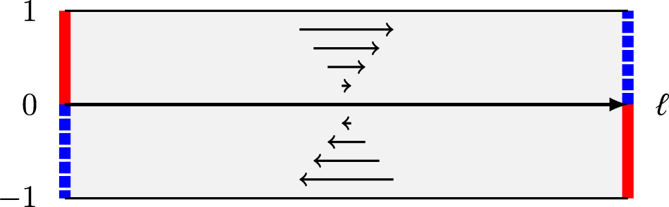
Let $\mathcal{X}=(0,\ell )$ , $\ell >0$ , denote the spatial domain. We write $L^p(\mathcal{X})$ , $W^{k,p}(\mathcal{X})$ , $H^k(\mathcal{X})$ for the usual Sobolev spaces defined on $\mathcal{X}$ . Similar notation is used for functions defined on other domains. Scalar products will be denoted by $⟨a,b{⟩}_S={\int }_{S}ab\mathrm{d}s$ . The range of velocities is $\mathcal{V}=(-1,1)$ and $\mathcal{Q}=\mathcal{X}\times \mathcal{V}$ describes the phase space. Note that any function $\overline{f}\in L^p(\mathcal{X})$ can be interpreted as a function $f\in L^p(\mathcal{Q})$ by constant extension $f(x,v)=\overline{f}(x)$ . The bar symbol is used throughout to indicate that functions do not depend on velocity $v$ . The same symbol is used for the velocity average of a function $f\in L^p(\mathcal{Q})$ , i.e.,

$$\overline{f}=\frac{1}{2}{\int }_{\mathcal{V}}f(v)\mathrm{d}v.$$

Following Dautray and Lions (1993), in- and outflow boundaries of the phase space $\mathcal{Q}$ are defined by

$${\mathrm{\Gamma }}^{\mathrm{in}}=\{0\}\times (0,1)\cup \{\ell \}\times (-1,0)\text{and}{\mathrm{\Gamma }}^{\mathrm{out}}=\{0\}\times (-1,0)\cup \{\ell \}\times (0,1);$$

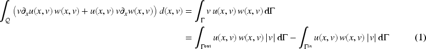
and $\mathrm{\Gamma }={\mathrm{\Gamma }}^{\mathrm{in}}\cup {\mathrm{\Gamma }}^{\mathrm{out}}$ is set; see Figure 1 for an illustration. By the product rule for differentiation and the fundamental theorem of calculus, one can see that

$$\begin{array}{rl}{\int }_{\mathcal{Q}}(v{\mathrm{\partial }}_{x}u(x,v)w(x,v)+u(x,v)v{\mathrm{\partial }}_{x}w(x,v))d(x,v)& ={\int }_{\mathrm{\Gamma }}vu(x,v)w(x,v)\mathrm{d}\mathrm{\Gamma }\\ & ={\int }_{{\mathrm{\Gamma }}^{\mathrm{out}}}u(x,v)w(x,v)|v|\mathrm{d}\mathrm{\Gamma }-{\int }_{{\mathrm{\Gamma }}^{in}}u(x,v)w(x,v)|v|\mathrm{d}\mathrm{\Gamma }\end{array}$$

(1)

for sufficiently smooth functions $u,w$ defined on $\mathcal{Q}$ . We write $L^p(\mathrm{\Gamma };|v|\mathrm{d}\mathrm{\Gamma })$ for the space of functions defined on $\mathrm{\Gamma }$ whose $p$ ^th power is integrable with respect to the measure $|v|\mathrm{d}\mathrm{\Gamma }$ . Given $T>0$ , $L^p(0,T;Y)$ and $W^{k,p}(0,T;Y)$ denote the Bochner spaces of functions defined on $(0,T)$ with values in some Banach space $Y$ equipped with the usual norms; see Evans (2010) for instance. For brevity, sometimes $L^p(Y)$ is written for $L^p(0,T;Y)$ , when the meaning is clear from the context. The spaces $C^k([0,T];Y)$ consists of all functions which are $k$ -times continuously differentiable with respect to time.

Figure 1.

Phase space $\mathcal{Q}=\mathcal{X}\times \mathcal{V}$ and in-/outflow boundaries ${\mathrm{\Gamma }}^{in}$ , ${\mathrm{\Gamma }}^{\mathrm{out}}$ depicted in (red, solid) and (blue, dotted), respectively.

2.2. Model Problem and Main Assumptions

The differential equations governing the kinetic chemotaxis model to be considered in the rest of the manuscript assumes a specific choice of the turning kernel and are given by Chalub et al. (2004); Othmer and Hillen (2002)

$$\begin{array}{rlr}{\epsilon }^2{\mathrm{\partial }}_t{u}^{\epsilon }+\epsilon v{\mathrm{\partial }}_x{u}^{\epsilon }+\sigma (u^{\epsilon }-{\overline{u}}^{\epsilon })& =\epsilon \alpha v{\mathrm{\partial }}_x{\overline{c}}^{\epsilon }{\overline{u}}^{\epsilon }& \text{in }\mathcal{Q}\times (0,T),\end{array}$$

(2)

$$\begin{array}{rlr}{\mathrm{\partial }}_t{\overline{c}}^{\epsilon }-D{\mathrm{\partial }}_{xx}{\overline{c}}^{\epsilon }+\beta {\overline{c}}^{\epsilon }& =\gamma {\overline{u}}^{\epsilon }& \text{in }\mathcal{X}\times (0,T).\end{array}$$

(3)

Recall that ${\overline{u}}^{\epsilon }=\frac{1}{2}{\int }_{\mathcal{V}}{u}^{\epsilon }(x,v)\mathrm{d}v$ denotes the velocity average of the population density $u^{\epsilon }$ , whereas the concentration ${\overline{c}}^{\epsilon }$ does not depend on $v$ naturally. The two equations are complemented by the boundary and initial conditions

$$\begin{array}{rlr}{u}^{\epsilon }& ={\overline{g}}_u\text{on }{\mathrm{\Gamma }}^{\mathrm{in}}\times (0,T),& u^{\epsilon }(0)={\overline{u}}_0\text{on }\mathcal{Q},\end{array}$$

(4)

$$\begin{array}{rlr}{\overline{c}}^{\epsilon }& ={\overline{g}}_c\text{on }\mathrm{\partial }\mathcal{X}\times (0,T),& {\overline{c}}^{\epsilon }(0)={\overline{c}}_0\text{on }\mathcal{X}.\end{array}$$

(5)

The boundary and initial data are thus chosen independently of the velocity $v$ . This facilitates the analysis in the asymptotic regime but could be relaxed to $g_u^{\epsilon }={\overline{g}}_u+\epsilon g_u^v$ and $u_0^{\epsilon }={\overline{u}}_0+\epsilon u_0^v$ with functions $g_u^v,u_0^v$ of order $\mathcal{O}$ (1) in $\epsilon$ that are $L^2$ in $v$ and satisfy similar assumptions as ${\overline{g}}_u,{\overline{u}}_0$ . The presented argumentation considers different time horizons $0<T\le T^{*}$ and asymptotic parameters $0<\epsilon \le {\epsilon }^{*}$ with $T^{*},{\epsilon }^{*}>0$ fixed, and makes use of the following assumptions which provide existence of sufficiently regular classical solutions to the model (2) to (5) that then allow the derivation of quantitative convergence rates.

Assumption 1

The parameters $\alpha ,\beta ,\gamma \ge 0$ and $D,{\epsilon }^{*},T^{*}>0$ are given constants. Furthermore $\sigma \in L^{\mathrm{\infty }}(\mathcal{X})$ with $0<{\sigma }_{min}\le \sigma (x)\le {\sigma }_{max}$ for a.a. $x\in \mathcal{X}$ . The initial data satisfy ${\overline{u}}_0\in H^2(\mathcal{X})$ , ${\overline{c}}_0\in H^4(\mathcal{X})$ , and the two boundary data ${\overline{g}}_u,{\overline{g}}_c\in W^{2,\mathrm{\infty }}(0,T^{*};{\mathbb{R}}^2)$ . The same notation ${\overline{g}}_u,{\overline{g}}_c$ is used for the linear extensions w.r.t. $x$ of the boundary data to functions ${\overline{g}}_u,{\overline{g}}_c\in W^{2,\mathrm{\infty }}(0,T^{*};W^{2,\mathrm{\infty }}(\mathcal{X}))$ . In addition, the compatibility conditions ${\overline{g}}_u(0)={\overline{u}}_0$ , ${\overline{g}}_c(0)={\overline{c}}_0$ , and ${\mathrm{\partial }}_t{\overline{g}}_c(0)=D{\mathrm{\partial }}_{xx}{\overline{c}}_0-\beta {\overline{c}}_0+\gamma {\overline{u}}_0$ are required to hold for $x\in \mathrm{\partial }\mathcal{X}$ .

2.3. Main Results

Under the above conditions, existence of a unique regular solution of the problem can be established and corresponding a priori bounds can be derived. Their explicit dependence on the parameter $\epsilon$ will be of importance for the asymptotic analysis later on.

Theorem 2

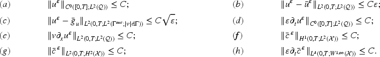
Let Assumption 1 hold. Then, there exists a time horizon $0<T\le T^{*}$ such that for any $0<\epsilon \le {\epsilon }^{*}$ the system (2) to (5) has a unique solution

$$\begin{array}{rl}{u}^{\epsilon }& \in C^1([0,T];L^2(\mathcal{Q}))\text{with}v{\mathrm{\partial }}_x{u}^{\epsilon }\in C^0([0,T];L^2(Q)),\\ {\overline{c}}^{\epsilon }& \in H^2(0,T;L^2(\mathcal{X}))\cap H^1(0,T;H^2(\mathcal{X})).\end{array}$$

Moreover, the following a priori bounds hold with a uniform constant $C>0$ :

$$\begin{array}{rlrlrlrl}& (a)& & \Vert u^{\epsilon }{\Vert }_{C^0([0,T];L^2(\mathcal{Q}))}\le C;& & (b)& & \Vert u^{\epsilon }-{\overline{u}}^{\epsilon }{\Vert }_{L^2(0,T;L^2(\mathcal{Q}))}\le C\epsilon ;\\ & (c)& & \Vert u^{\epsilon }-{\overline{g}}_u{\Vert }_{L^2(0,T;L^2({\mathrm{\Gamma }}^{out};|v|\mathrm{d}\mathrm{\Gamma }))}\le C\sqrt{\epsilon };& & (d)& & \Vert \epsilon {\mathrm{\partial }}_t{u}^{\epsilon }{\Vert }_{C^0([0,T];L^2(\mathcal{Q}))}\le C;\\ & (e)& & \Vert v{\mathrm{\partial }}_x{u}^{\epsilon }{\Vert }_{L^2(0,T;L^2(\mathcal{Q}))}\le C;& & (f)& & \Vert {\overline{c}}^{\epsilon }{\Vert }_{H^1(0,T;L^2(\mathcal{X}))}\le C;\\ & (g)& & \Vert {\overline{c}}^{\epsilon }{\Vert }_{L^2(0,T;H^2(\mathcal{X}))}\le C;& & (h)& & \Vert \epsilon {\mathrm{\partial }}_t{\overline{c}}^{\epsilon }{\Vert }_{L^4(0,T;W^{1,\mathrm{\infty }}(\mathcal{X}))}\le C.\end{array}$$

The existence of a unique solution will be established via fixed-point arguments and results about the linearized evolution problems corresponding to the two differential equations. The bounds for the solution are derived by careful energy estimates and interpolation arguments. The detailed proof is presented in Section 3.

The second main result of the paper is concerned with the behavior of solutions in the asymptotic limit $\epsilon \to 0$ . The main findings can be summarized as follows.

Theorem 3

Let Assumption 1 hold and $(u^{\epsilon },{\overline{c}}^{\epsilon })$ be the solutions of (2) to (5) on $[0,T]$ , as provided by Theorem 2, for a sequence $\epsilon \to 0$ . Then $u^{\epsilon }\rightharpoonup {\overline{u}}^0$ weakly in $L^2(0,T;L^2(\mathcal{Q}))$ and ${\overline{c}}^{\epsilon }\to {\overline{c}}^0$ in $L^2(0,T;H^1(\mathcal{X}))$ , where $({\overline{u}}^0,{\overline{c}}^0)$ is the unique weak solution of the Keller–Segel system

$$\begin{array}{rl}{\mathrm{\partial }}_t{\overline{u}}^0-{\mathrm{\partial }}_x(\overline{\mu }{\mathrm{\partial }}_x{\overline{u}}^0-\overline{\chi }{\mathrm{\partial }}_x{\overline{c}}^0{\overline{u}}^0)=0& \text{in }\mathcal{X}\times (0,T),\end{array}$$

(6)

$$\begin{array}{rl}{\mathrm{\partial }}_t{\overline{c}}^0-D{\mathrm{\partial }}_{xx}{\overline{c}}^0+\beta {\overline{c}}^0=\gamma {\overline{u}}^0& \text{in }\mathcal{X}\times (0,T),\end{array}$$

(7)

with motility and chemotactic coefficient

$$\overline{\mu }(x)=\sigma {(x)}^{-1}\frac{1}{2}{\int }_{\mathcal{V}}{v}^2\mathrm{d}v\text{and}\overline{\chi }(x)=\alpha \overline{\mu }(x),$$

(8)

and with boundary and initial conditions

$$\begin{array}{rlr}{\overline{u}}^0& ={\overline{g}}_u\text{on }\mathrm{\partial }\mathcal{X}\times (0,T),& {\overline{u}}^0(0)={\overline{u}}_0\text{on }\mathcal{X},\end{array}$$

(9)

$$\begin{array}{rlr}{\overline{c}}^0& ={\overline{g}}_c\text{on }\mathrm{\partial }\mathcal{X}\times (0,T),& {\overline{c}}^0(0)={\overline{c}}_0\text{on }\mathcal{X}.\end{array}$$

(10)

If, in addition, $\sigma \in W^{1,\mathrm{\infty }}(\mathcal{X})$ , then the asymptotic error is bounded by

$$\Vert u^{\epsilon }-{\overline{u}}^0{\Vert }_{L^{\mathrm{\infty }}(0,T;L^2(\mathcal{Q}))}+\Vert {\overline{c}}^{\epsilon }-{\overline{c}}^0{\Vert }_{L^{\mathrm{\infty }}(0,T;H^1(\mathcal{X}))}\le C\epsilon$$

(11)

with a constant $C$ that can be chosen independent of $\epsilon$ .

The verification of the above assertions relies on the a priori bounds of Theorem 2, the extraction of convergent subsequences, a weak characterization of solutions to the limit system, and an extension of the arguments used in Egger and Schlottbom (2012, 2014) for the analysis of the radiative transfer equation. The detailed proof of Theorem 3 is presented in Sections 4 and 5.

Remark 4

The presented results are local in time. From the global well-posedness of the limit problem in one space dimension, one would expect that they should be valid for $T=\mathrm{\infty }$ . However, a different analysis as the one presented below would be required to establish global existence of the kinetic model and to exclude finite time blow-up due to the quadratic non-linearity. The same challenges appear in the limit problem, and could be addressed by additionally establishing positivity of solutions and proving uniform $L^1$ -bounds as in Egger and Schöbel-Kröhn (2020); Toshitaka Nagai and Yoshida (1997). Another way to obtain global-in-time results is to replace the nonlinear coupling term in (2) by $\epsilon \alpha v\mathrm{\Psi }({\mathrm{\partial }}_x{\overline{c}}^{\epsilon }){\overline{u}}^{\epsilon }$ for a suitable bounded function $\mathrm{\Psi }$ , which acts as flux limiting. Such models were recently introduced to avoid nonphysical blow-up behavior and were shown to attain global solutions (Perthame et al., 2019); also see Bellomo and Winkler (2017); Burger et al. (2006) for the related analysis of the flux-limited Keller–Segel model in multiple space dimensions. The analysis presented in the next section can be generalized to this case, and the estimates of Theorems 2 and 3 then hold globally in time.

3. Proof of Theorem 2

The existence of a unique solution to (2) to (5) will be proven by constructing a fixed-point of the mapping $\mathrm{\Phi }:z\mapsto u$ , where $(u,\overline{c})$ solves the linearized equations

$$\begin{array}{rl}{\epsilon }^2{\mathrm{\partial }}_{t}u+\epsilon v{\mathrm{\partial }}_{x}u+\sigma (u-\overline{u})=\epsilon \alpha v{\mathrm{\partial }}_x\overline{c}\overline{z}& \text{in }\mathcal{Q}\times (0,T),\end{array}$$

(12)

$$\begin{array}{rl}{\mathrm{\partial }}_t\overline{c}-D{\mathrm{\partial }}_{xx}\overline{c}+\beta \overline{c}=\gamma \overline{z}& \text{in }\mathcal{X}\times (0,T),\end{array}$$

(13)

together with the boundary and initial conditions (4) and (5), now required for $u$ and $\overline{c}$ instead of $u^{\epsilon }$ and ${\overline{c}}^{\epsilon }$ . Also recall that $\overline{z}=\frac{1}{2}{\int }_{\mathcal{V}}z(\cdot ,v)dv$ denotes the velocity average. Before proving the assertions of Theorem 2, some preliminary results about the two linear problems (12) and (13) defining $\overline{c}$ and $u$ are collected. Throughout the proofs, $C_i$ and $C_i^{\prime }$ denote constants that only depend on the problem data, in particular, the upper bounds ${\epsilon }^{*}$ , $T^{*}$ for the asymptotic parameter and the time horizon.

3.1. Linearized Diffusion Equation

An application of standard results for parabolic differential equations provides the following statements.

Proposition 5

Let Assumption 1 hold. Then, for any $0<T\le T^{*}$ and for $z\in C^1([0,T];L^2(Q))$ with $z(0)={\overline{u}}_0$ , Equation (13) has a unique solution $\overline{c}$ , additionally satisfying the initial and boundary conditions $\overline{c}(0)={\overline{c}}_0$ on $\mathcal{X}$ and $\overline{c}={\overline{g}}_c$ on $\mathrm{\partial }\mathcal{X}\times (0,T)$ . Moreover, for any $p<\mathrm{\infty }$ ,

$$\begin{array}{rl}\Vert \overline{c}{\Vert }_{W^{1,p}(0,T;L^2(\mathcal{X}))}+\Vert \overline{c}{\Vert }_{L^p(0,T;H^2(\mathcal{X}))}& \le C_1+C_2\Vert \overline{z}{\Vert }_{L^p(0,T;L^2(\mathcal{X}))}\\ \Vert {\mathrm{\partial }}_t\overline{c}{\Vert }_{W^{1,p}(0,T;L^2(\mathcal{X}))}+\Vert {\mathrm{\partial }}_t\overline{c}{\Vert }_{L^p(0,T;H^2(\mathcal{X}))}& \le C_1+C_2\Vert {\mathrm{\partial }}_t\overline{z}{\Vert }_{L^p(0,T;L^2(\mathcal{X}))}\end{array}$$

with $C_1,C_2$ depending only on $p$ and the bounds for the problem data in Assumption 1. In the case that ${\overline{g}}_u,{\overline{g}}_c,{\overline{c}}_0,{\overline{u}}_0\equiv 0$ , one can choose $C_1=0$ .

Proof.

The function $\overline{d}=\overline{c}-{\overline{g}}_c$ satisfies

$$\begin{array}{rl}{\mathrm{\partial }}_t\overline{d}-D{\mathrm{\partial }}_{xx}\overline{d}+\beta \overline{d}=\overline{f}& \text{in }\mathcal{X}\times (0,T),\end{array}$$

(14)

$$\begin{array}{rl}\overline{d}(0)={\overline{d}}_0& \text{on }\mathcal{X},\end{array}$$

(15)

with $\overline{f}=\gamma \overline{z}-{\mathrm{\partial }}_t{\overline{g}}_c-\beta {\overline{g}}_c$ , ${\overline{d}}_0={\overline{c}}_0-{\overline{g}}_c(0)$ , and $\overline{d}=0$ on $\mathrm{\partial }\mathcal{X}\times (0,T)$ . The conditions of Assumption 1 show that $\overline{f}\in L^p(0,T;L^2(\mathcal{X}))$ and ${\overline{d}}_0\in H_0^1(\mathcal{X})\cap H^2(\mathcal{X})$ . Existence of a unique solution $\overline{c}\in W^{1,p}(0,T;L^2(\mathcal{X}))\cap L^p(0,T;H^2(\mathcal{X}))$ and the first bound then follow from known maximal parabolic regularity of the heat equation; see Augner (2024); Dore (1993). By formally differentiating (13) in time, one sees that $\overline{d}={\mathrm{\partial }}_t\overline{c}-{\mathrm{\partial }}_t{\overline{g}}_c$ also satisfies (14) and (15), now with $\overline{f}=\gamma {\mathrm{\partial }}_t\overline{z}-{\mathrm{\partial }}_{tt}{\overline{g}}_c-\beta {\mathrm{\partial }}_t{\overline{g}}_c$ and ${\overline{d}}_0=D{\mathrm{\partial }}_{xx}{\overline{c}}_0-\beta {\overline{c}}_0+\gamma {\overline{u}}_0-{\mathrm{\partial }}_t{\overline{g}}_c(0)$ . By Assumption 1 and the regularity of $\overline{z}$ , bounds for ${\overline{d}}_0\in H_0^1(\mathcal{X})\cap H^2(\mathcal{X})$ and $\overline{f}\in L^p(0,T;L^2(\mathcal{X}))$ can be established, which leads to the estimate for the time derivatives.

3.2. Linearized Kinetic Equation

As a next step, existence of a unique solution to (12) is established for appropriate boundary and initial conditions. The functions $\overline{c}$ , $\overline{z}$ are assumed assumed given at this point.

Proposition 6

Let Assumption 1 hold and let $0<T\le T^{*}$ . Then for any $z\in C^1([0,T];L^2(\mathcal{Q}))$ and $\overline{c}$ as given by Proposition 5, Equation (12) has a unique solution $u\in C^1([0,T];L^2(\mathcal{Q}))$ with derivative $v{\mathrm{\partial }}_{x}u\in C^0([0,T];L^2(\mathcal{Q}))$ , satisfying $u(0)={\overline{u}}_0$ on $\mathcal{Q}$ and $u={\overline{g}}_u$ on ${\mathrm{\Gamma }}^{in}\times (0,T)$ .

Proof.

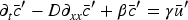
Similar to before, define $w=u-{\overline{g}}_u$ , which can be seen to satisfy

$$\begin{array}{rl}{\epsilon }^2{\mathrm{\partial }}_{t}w+\epsilon v{\mathrm{\partial }}_{x}w+\sigma (w-\overline{w})=\epsilon v{\overline{f}}_1+{\epsilon }^2{\overline{f}}_2& \text{in }\mathcal{Q}\times (0,T),\end{array}$$

(16)

$$\begin{array}{rl}w(0)={\overline{w}}_0& \text{on }\mathcal{Q},\end{array}$$

(17)

with ${\overline{f}}_1=\alpha {\mathrm{\partial }}_x\overline{c}\overline{z}-{\mathrm{\partial }}_x{\overline{g}}_u$ , ${\overline{f}}_2=-{\mathrm{\partial }}_t{\overline{g}}_u$ , ${\overline{w}}_0={\overline{u}}_0-{\overline{g}}_u(0)$ , and homogeneous inflow boundary conditions $w=0$ on ${\mathrm{\Gamma }}^{\mathrm{in}}\times (0,T)$ . This can be written as an abstract Cauchy problem

$$\begin{array}{rl}{\mathrm{\partial }}_{t}w+{\mathcal{A}}^{\epsilon }w& =f,t>0,\end{array}$$

(18)

$$\begin{array}{rl}w(0)& ={\overline{w}}_0,\end{array}$$

(19)

on the Hilbert space $\mathcal{H}=L^2(\mathcal{Q})$ , with right hand side $f=\frac{1}{\epsilon }v{\overline{f}}_1+{\overline{f}}_2$ , and densely defined linear operator ${\mathcal{A}}^{\epsilon }:D({\mathcal{A}}^{\epsilon })\subset \mathcal{H}\to \mathcal{H}$ , ${\mathcal{A}}^{\epsilon }w=\frac{1}{\epsilon }v{\mathrm{\partial }}_{x}w+\frac{\sigma }{{\epsilon }^2}(w-\overline{w})$ with domain

$$D({\mathcal{A}}^{\epsilon })=\{w\in L^2(\mathcal{Q}):v{\mathrm{\partial }}_{x}w\in L^2(\mathcal{Q}),w{|}_{{\mathrm{\Gamma }}^{\mathrm{in}}}=0\}.$$

Note that $D({\mathcal{A}}^{\epsilon })\subset \mathcal{H}$ is dense and (1) shows that

$$⟨{\mathcal{A}}^{\epsilon }w,w{⟩}_{\mathcal{Q}}=\frac{1}{\epsilon }⟨v{\mathrm{\partial }}_{x}w,w{⟩}_{\mathcal{Q}}+\frac{1}{{\epsilon }^2}⟨\sigma (w-\overline{w}),w{⟩}_{\mathcal{Q}}\ge 0,$$

for all $w\in D({\mathcal{A}}^{\epsilon })$ , where $⟨a,b{⟩}_{\mathcal{Q}}={\int }_{\mathcal{Q}}abd(x,v)$ ; this shows that $-{\mathcal{A}}^{\epsilon }$ is dissipative (Cazenave & Haraux, 1998, Prop. 2.4.2). From Agoshkov (1998, Thm. 3.5), one can deduce that for any $\lambda >0$ and $f\in L^2(\mathcal{Q})$ , the equation ${\mathcal{A}}^{\epsilon }w+\lambda w=f$ has a unique solution $w\in D({\mathcal{A}}^{\epsilon })$ , and one concludes that $-{\mathcal{A}}^{\epsilon }$ is m-dissipative. Hence $-{\mathcal{A}}^{\epsilon }$ generates a strongly continuous semigroup of contractions (Cazenave & Haraux, 1998, Thm. 3.4.4). From the assumptions, one further sees that ${\overline{w}}_0\in D({\mathcal{A}}^{\epsilon })$ and $f\in W^{1,1}(0,T;\mathcal{H})$ , which implies the existence of a unique classical solution $w\in C^1([0,T];\mathcal{H})\cap C^0([0,T];D({\mathcal{A}}^{\epsilon }))$ to (18) and (19); see e.g. Cazenave and Haraux (1998, Prop. 4.1.6). The function $u=w+{\overline{g}}_u$ then is a sufficiently regular solution of (12) satisfying the required initial and boundary conditions. Uniqueness follows from the linearity of the problem.

Remark 7

Since $-{\mathcal{A}}^{\epsilon }$ generates a semigroup of contractions, one also obtains the bounds

$$\Vert w{\Vert }_{C([0,T];L^2(Q))}\le \Vert {\overline{w}}_0{\Vert }_{L^2(\mathcal{Q})}+\Vert f{\Vert }_{L^1(0,T;L^2(\mathcal{Q}))}.$$

Inserting $f=\frac{1}{\epsilon }v{\overline{f}}_1+{\overline{f}}_2$ shows that this simple estimate is, however, not uniform in $\epsilon$ . A refined analysis is thus required to obtain sharper a priori bounds.

3.3. A priori Bounds for Linearized Equations

As a next step, additional bounds for the solution $(u,c)$ of (12) and (13) are derived, making explicit the dependence on $\epsilon$ . To do so, we assume $z\in C^1([0,T];L^2(\mathcal{Q}))$ is given with $z(0)={\overline{u}}_0$ and define the weighted norm

$$\Vert z{\Vert }_{\epsilon ,T}^2=\Vert z{\Vert }_{L^{\mathrm{\infty }}(0,T;L^2(\mathcal{Q}))}^2+{\epsilon }^2\Vert {\mathrm{\partial }}_{t}z{\Vert }_{L^{\mathrm{\infty }}(0,T;L^2(\mathcal{Q}))}^2\le C_z^2.$$

(20)

By careful application of the estimates of Proposition 5 and additional energy estimates for the linearized kinetic equation (12), the following assertions are obtained.

Proposition 8

Let $0<\epsilon \le {\epsilon }^{*}$ , $C_z\ge 1$ and $0<T\le min(1,T^{*})$ be given. Then for every $z\in C^1([0,T];L^2(\mathcal{Q}))$ with $z(0)={\overline{u}}_0$ that is bounded according to (20), the solution $(\overline{u},\overline{c})$ of (12) and (13) satisfies the bounds of Theorem 2 with a constant $C$ that only depends on the bounds for the problem data in Assumption 1 and $C_z$ .

Proof.

The estimates (f) to (h) of Theorem 2 for the function $\overline{c}$ follow readily from Proposition 5. To derive the improved bounds for $u$ , Equation (16) is tested with $w/{\epsilon }^2$ .

Using the integration-by-parts formula (1) shows that

$$\begin{array}{rl}& \frac{1}{2}\frac{\mathrm{d}}{\mathrm{d}t}\Vert w{\Vert }_{L^2(\mathcal{Q})}^2+\frac{1}{2\epsilon }\Vert w{\Vert }_{L^2({\mathrm{\Gamma }}^{\mathrm{out}};|v|\mathrm{d}\mathrm{\Gamma })}^2+\frac{1}{{\epsilon }^2}\Vert \sqrt{\sigma }(w-\overline{w}){\Vert }_{L^2(\mathcal{Q})}^2\\ & =\frac{1}{\epsilon }(v{\overline{f}}_1,w-\overline{w}{)}_{L^2(\mathcal{Q})}+({\overline{f}}_2,w{)}_{L^2(\mathcal{Q})}\\ & \le \frac{1}{2{\sigma }_{\min }}\Vert {\overline{f}}_1{\Vert }_{L^2(\mathcal{X})}^2+\frac{1}{2{\epsilon }^2}\Vert \sqrt{\sigma }(w-\overline{w}){\Vert }_{L^2(\mathcal{Q})}^2+\Vert {\overline{f}}_2{\Vert }_{L^2(\mathcal{X})}^2+\frac{1}{2}\Vert w{\Vert }_{L^2(\mathcal{Q})}^2.\end{array}$$

The second term on the right hand side can be absorbed into the left hand side of this inequality. By application of Grönwall’s inequality, one immediately obtains

$$\begin{array}{rl}& \Vert w{\Vert }_{L^{\mathrm{\infty }}(0,T;L^2(\mathcal{Q}))}^2+\frac{1}{\epsilon }\Vert w{\Vert }_{L^2(0,T;L^2({\mathrm{\Gamma }}^{\mathrm{out}};|v|\mathrm{d}\mathrm{\Gamma }))}^2+\frac{{\sigma }_{\min }}{{\epsilon }^2}\Vert w-\overline{w}{\Vert }_{L^2(0,T;L^2(\mathcal{Q}))}^2\end{array}$$

(21)

$$\begin{array}{rl}& \le e^T(\Vert w(0){\Vert }_{L^2(\mathcal{Q})}^2+\frac{1}{{\sigma }_{\min }}\Vert {\overline{f}}_1{\Vert }_{L^2(0,T;L^2(\mathcal{X}))}^2+2\Vert {\overline{f}}_2{\Vert }_{L^2(0,T;L^2(\mathcal{X}))}^2).\end{array}$$

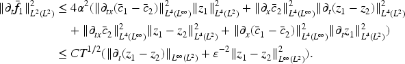
From $w(0)={\overline{u}}_0-{\overline{g}}_u(0)$ and the assumptions, one obtains $\Vert \overline{w}(0){\Vert }_{L^2(\mathcal{Q})}\le C_0$ . Using Hölder and Young inequalities, one can further estimate

$$\begin{array}{rl}\Vert {\overline{f}}_1{\Vert }_{L^2(0,T;L^2(\mathcal{X}))}^2& \le 2{\alpha }^2\Vert {\mathrm{\partial }}_x\overline{c}{\Vert }_{L^4(0,T;L^{\mathrm{\infty }}(\mathcal{X}))}^2\Vert \overline{z}{\Vert }_{L^4(0,T;L^2(\mathcal{X}))}^2+2\Vert {\mathrm{\partial }}_x{\overline{g}}_u{\Vert }_{L^2(0,T;L^2(\mathcal{X}))}^2\\ & \le C_1{C}_z^4{T}^{1/2}+C_2.\end{array}$$

The last bound follows from previous estimates for $\overline{c}$ , the assumptions on the problem data, and the estimate $\Vert a{\Vert }_{L^4(0,T)}\le T^{1/4}\Vert a{\Vert }_{L^{\mathrm{\infty }}(0,T)}$ , which again is a consequence of Hölder’s inequality. The definition of ${\overline{f}}_2$ implies that $\Vert {\overline{f}}_2{\Vert }_{L^2(0,T;L^2(\mathcal{X}))}=\Vert {\mathrm{\partial }}_t{\overline{g}}_u{\Vert }_{L^2(0,T;L^2(\mathcal{X}))}\le C_3$ . Note that the constants $C_i$ can be chosen independently of $\epsilon$ and $T$ .

The estimates (a) to (c) in Theorem 2 for the function $u={\overline{g}}_u+w$ then follow from the triangle inequality. The remaining bounds are established by a consideration of a formal differentiation of (16) and (17). Then $w^{\prime }={\mathrm{\partial }}_{t}w={\mathrm{\partial }}_{t}u-{\mathrm{\partial }}_t{\overline{g}}_u$ is a mild solution of

$$\begin{array}{rl}{\epsilon }^2{\mathrm{\partial }}_t{w}^{\prime }+\epsilon v{\mathrm{\partial }}_x{w}^{\prime }+\sigma (w^{\prime }-{\overline{w}}^{\prime })& =\epsilon v{\overline{f}}_1^{\prime }+{\epsilon }^2{\overline{f}}_2^{\prime },\\ w^{\prime }(0)& =w_0^{\prime },\end{array}$$

with ${\overline{f}}_1^{\prime }=\alpha {\mathrm{\partial }}_{tx}\overline{c}\overline{z}+\alpha {\mathrm{\partial }}_x\overline{c}{\mathrm{\partial }}_t\overline{z}-{\mathrm{\partial }}_{tx}{\overline{g}}_u$ , ${\overline{f}}_2^{\prime }=-{\mathrm{\partial }}_{tt}{\overline{g}}_u$ , and $w_0^{\prime }={\epsilon }^{-1}v(\alpha {\mathrm{\partial }}_x{\overline{c}}_0{\overline{u}}_0-{\mathrm{\partial }}_x{\overline{u}}_0)-{\mathrm{\partial }}_t{\overline{g}}_u(0)$ . By the assumptions, one has $\Vert \epsilon w_0^{\prime }{\Vert }_{L^2(\mathcal{Q})}\le C_0$ and $\Vert {\overline{f}}_2^{\prime }{\Vert }_{L^2(L^2)}^2=\Vert {\mathrm{\partial }}_{tt}{\overline{g}}_u{\Vert }_{L^2(L^2)}^2\le C_3$ . By similar arguments as used before, it can further be shown that

$$\begin{array}{rl}\Vert {\overline{f}}_1^{\prime }{\Vert }_{L^2(L^2)}^2& \le 3{\alpha }^2(\Vert {\mathrm{\partial }}_{tx}\overline{c}{\Vert }_{L^4(L^{\mathrm{\infty }})}^2\Vert \overline{z}{\Vert }_{L^4(L^2)}^2+\Vert {\mathrm{\partial }}_x\overline{c}{\Vert }_{L^4(L^{\mathrm{\infty }})}^2\Vert {\mathrm{\partial }}_t\overline{z}{\Vert }_{L^4(L^2)}^2)+3\Vert {\mathrm{\partial }}_{tx}{\overline{g}}_u{\Vert }_{L^2(L^2)}^2\\ & \le C_1{C}_z^4{\epsilon }^{-2}{T}^{1/2}+C_2.\end{array}$$

An application of the energy estimate (21) to $w^{\prime }={\mathrm{\partial }}_{t}w$ then yields $\Vert \epsilon {\mathrm{\partial }}_{t}w{\Vert }_{L^{\mathrm{\infty }}(L^2)}^2\le C$ . By rearranging (16) and using the previous bounds, one further obtains $\Vert v{\mathrm{\partial }}_{x}w{\Vert }_{L^2(L^2(\mathcal{Q}))}\le C^{\prime }$ . The estimates (a), (b) and (d), (e) of Theorem 2 for $u=w+{\overline{g}}_u$ then follow by the triangle inequality and the assumptions on the problem data.

3.4. Existence of a Unique Solution

As noted in the beginning of Section 3, a fixed-point argument will be used to establish existence of a solution to the system (2) to (5). To this end, fix a $C_z$ sufficiently large and denote by $\mathrm{\Phi }:{\mathcal{S}}_T\to C^1([0,T];L^2(\mathcal{Q}))$ , $z\mapsto u$ the mapping that assigns to a given $z$ in

$${\mathcal{S}}_T=\{z\in C^1([0,T];L^2(\mathcal{Q})):\Vert z{\Vert }_{\epsilon ,T}\le C_z,z(0)={\overline{u}}_0\}$$

(22)

the solution $u$ of the linearized Equations (12) and (13) with the required initial and boundary conditions. Propositions 5 and 6 show that this mapping is well-defined. The goal is to show that $\mathrm{\Phi }$ is a self-mapping and a contraction on ${\mathcal{S}}_T$ whenever $0<T\le T^{*}$ is chosen small enough in relation to $C_z$ . Note that choosing $C_z$ sufficiently large will also ensure that ${\mathcal{S}}_T$ is non-empty.

Step 1. Let $z\in {\mathcal{S}}_T$ and $(u,\overline{c})$ denote the solution of (12) and (13). Further set $w=u-{\overline{g}}_u$ . Then from the estimates derived in the proof of Proposition 8, one sees that

$$\Vert u{\Vert }_{\epsilon ,T}^2\le 2\Vert {\overline{g}}_u{\Vert }_{\epsilon ,T}^2+2\Vert w{\Vert }_{\epsilon ,T}^2\le C_1{C}_z^4{T}^{1/2}+C_2$$

with constants $C_1$ , $C_2$ that can be chosen independent of $\epsilon$ and $T$ . By choosing $C_z\ge max(1,C_1+C_2)$ and $T\le min(T^{*},C_z^{-8})$ independent of $\epsilon$ , one obtains $\Vert u{\Vert }_{\epsilon ,T}\le C_z$ . Moreover, it is clear by construction that $u\in C^1([0,T];L^2(\mathcal{Q}))$ and it satisfies the required initial and boundary conditions. Hence $\mathrm{\Phi }$ is a self-mapping on ${\mathcal{S}}_T$ for this choice of $T$ and $C_z$ .

Step 2. Let $z_1,z_2\in {\mathcal{S}}_T$ be given and $(u_1,{\overline{c}}_1)$ , $(u_2,{\overline{c}}_2)$ be the corresponding solutions of the system (12) and (13) with the required initial and boundary conditions. Then the two functions $\overline{d}={\overline{c}}_1-{\overline{c}}_2$ and $w=u_1-u_2$ satisfy (14) and (16) with $\overline{f}=\gamma ({\overline{z}}_1-{\overline{z}}_2)$ , ${\overline{f}}_1=\alpha ({\mathrm{\partial }}_x{\overline{c}}_1{\overline{z}}_1-{\mathrm{\partial }}_x{\overline{c}}_2{\overline{z}}_2)$ , and ${\overline{f}}_2=0$ , and with homogeneous initial and boundary conditions. The estimates of Proposition 5 and the continuous embeddings of $H^1(\mathcal{X})\to L^{\mathrm{\infty }}(\mathcal{X})$ and $L^{\mathrm{\infty }}(0,T)\to L^4(0,T)$ show that

$$\begin{array}{rl}\Vert {\mathrm{\partial }}_x\overline{d}{\Vert }_{L^4(0,T;L^{\mathrm{\infty }}(\mathcal{X}))}& \le C\Vert z_1-z_2{\Vert }_{L^{\mathrm{\infty }}(0,T;L^2(\mathcal{Q}))}\\ \Vert {\mathrm{\partial }}_{tx}\overline{d}{\Vert }_{L^4(0,T;L^{\mathrm{\infty }}(\mathcal{X}))}& \le C\Vert {\mathrm{\partial }}_t{z}_1-{\mathrm{\partial }}_t{z}_2{\Vert }_{L^{\mathrm{\infty }}(0,T;L^2(\mathcal{Q}))}\end{array}$$

with a uniform constant $C$ independent of $\epsilon$ and $T$ . Using the a priori bounds on solutions of the linearized equations obtained so far, one can then further estimate

$$\begin{array}{rl}\Vert {\overline{f}}_1{\Vert }_{L^2(L^2)}^2& \le 2{\alpha }^2(\Vert {\mathrm{\partial }}_x{\overline{c}}_1-{\mathrm{\partial }}_x{\overline{c}}_2{\Vert }_{L^4(L^{\mathrm{\infty }})}^2\Vert {\overline{z}}_1{\Vert }_{L^4(L^2)}^2+\Vert {\mathrm{\partial }}_x{\overline{c}}_2{\Vert }_{L^4(L^{\mathrm{\infty }})}^2\Vert {\overline{z}}_1-{\overline{z}}_2{\Vert }_{L^4(L^2)}^2)\\ & \le C{T}^{1/2}\Vert {\overline{z}}_1-{\overline{z}}_2{\Vert }_{L^{\mathrm{\infty }}(0,T;L^2)}^2,\end{array}$$

and in a similar manner, one obtains

$$\begin{array}{rl}\Vert {\mathrm{\partial }}_t{\overline{f}}_1{\Vert }_{L^2(L^2)}^2& \le 4{\alpha }^2(\Vert {\mathrm{\partial }}_{tx}({\overline{c}}_1-{\overline{c}}_2){\Vert }_{L^4(L^{\mathrm{\infty }})}^2\Vert z_1{\Vert }_{L^4(L^2)}^2+\Vert {\mathrm{\partial }}_x{\overline{c}}_2{\Vert }_{L^4(L^{\mathrm{\infty }})}^2\Vert {\mathrm{\partial }}_t(z_1-z_2){\Vert }_{L^4(L^2)}^2\\ & +\Vert {\mathrm{\partial }}_{tx}{\overline{c}}_2{\Vert }_{L^4(L^{\mathrm{\infty }})}^2\Vert z_1-z_2{\Vert }_{L^4(L^2)}^2+\Vert {\mathrm{\partial }}_x({\overline{c}}_1-{\overline{c}}_2){\Vert }_{L^4(L^{\mathrm{\infty }})}^2\Vert {\mathrm{\partial }}_t{z}_1{\Vert }_{L^4(L^2)}^2)\\ & \le C{T}^{1/2}(\Vert {\mathrm{\partial }}_t(z_1-z_2){\Vert }_{L^{\mathrm{\infty }}(L^2)}+{\epsilon }^{-2}\Vert z_1-z_2{\Vert }_{L^{\mathrm{\infty }}(L^2)}^2).\end{array}$$

By combination of the estimates derived in the proof of Proposition 8, one thus obtains

$$\Vert u_1-u_2{\Vert }_{\epsilon ,T}^2\le C{e}^T{T}^{1/2}\Vert z_1-z_2{\Vert }_{\epsilon ,T}^2.$$

Note that $C$ is again independent of $\epsilon$ and $T$ but depends on $C_z$ . For $T<min\{1/(C^2{e}^{2T^{*}}),T^{*},C_z^{-8}\}$ , one further has $L=C{e}^T{T}^{1/2}<1$ . Hence $\mathrm{\Phi }$ is a contraction on ${\mathcal{S}}_T$ for this choice of $T$ .

Step 3. In summary, it was shown that $\mathrm{\Phi }$ is a self-mapping and a contraction on ${\mathcal{S}}_T$ whenever $C_z$ is chosen sufficiently large in absolute terms and $T$ sufficiently small in relation to $C_z$ . For $T>0$ , the set ${\mathcal{S}}_T$ is nonempty and closed. The existence of a unique fixed-point $u=\mathrm{\Phi }(u)$ in ${\mathcal{S}}_T$ then follows readily from Banach’s fixed-point theorem. In addition, any fixed-point of $\mathrm{\Phi }$ also is a solution of (2) to (5), and vice versa. This yields existence of a unique solution on $[0,T]$ .

3.5. A priori Bounds

By construction, $(u,\overline{c})$ also is a solution of the linearized equations (12) and (13) with $z=u$ and satisfying the required initial and boundary conditions. The bounds in Theorem 2 then follow immediately from the ones of Proposition 5 and Proposition 8. This concludes the proof of Theorem 2.

4. Proof of Theorem 3, Part 1

It is now shown that solutions $(u^{\epsilon },{\overline{c}}^{\epsilon })$ of the kinetic chemotaxis model (2) to (5) converge in an appropriate sense to the unique solution $({\overline{u}}^0,{\overline{c}}^0)$ of the Keller–Segel system (6) to (10).

4.1. Keller–Segel System

To begin, some properties about solutions to the limit system are summarized, which are required later on. A pair of functions $({\overline{u}}^0,{\overline{c}}^0)$ is called a weak solution, if

$$\begin{array}{rl}& {\overline{u}}^0\in L^2(0,T;H^1(\mathcal{X}))\cap H^1(0,T;H^{-1}(\mathcal{X})),\end{array}$$

(23)

$$\begin{array}{rl}& {\overline{c}}^0\in L^2(0,T;H^2(\mathcal{X}))\cap H^1(0,T;L^2(\mathcal{X})),\end{array}$$

(24)

satisfy (7) pointwise a.e., (9) and (10) in a trace sense and (6) in a weak sense, i.e.,

$$⟨{\mathrm{\partial }}_t{\overline{u}}^0,\overline{\varphi }{⟩}_{\mathcal{X}}+⟨\overline{\mu }{\mathrm{\partial }}_x{\overline{u}}^0-\overline{\chi }{\mathrm{\partial }}_x{\overline{c}}^0{\overline{u}}^0,{\mathrm{\partial }}_x\overline{\varphi }{⟩}_{\mathcal{X}}=0$$

(25)

for all $\overline{\varphi }\in H_0^1(\mathcal{X})$ and for a.a. $t\in (0,T)$ . Note that the solution components ${\overline{u}}^0$ , ${\overline{c}}^0$ here depend on time, while the test function is independent of time.

Proposition 9

Let Assumption 1 be valid. Then (6) to (10) has a unique weak solution. If, in addition, $\sigma \in W^{1,\mathrm{\infty }}(\mathcal{X})$ , then $\overline{\mu },\overline{\chi }$ as defined in (8) belong to $W^{1,\mathrm{\infty }}(\mathcal{X})$ and

$${\overline{u}}^0\in H^1(0,T;H^1(\mathcal{X}))\cap L^{\mathrm{\infty }}(0,T;H^2(\mathcal{X})).$$

Proof.

Existence of a unique local weak solution ${\overline{u}}^0\in L^2(0,T^{*};H^1(\mathcal{X}))\cap H^1(0,T^{*};H^{-1}(\mathcal{X}))$ and ${\overline{c}}^0\in L^2(0,T^{*};H^2(\mathcal{X}))\cap H^1(0,T^{*};L^2(\mathcal{X}))$ up to some time $T^{*}>0$ depending only on the problem data has been proven in Egger and Schöbel-Kröhn (2020). Further note that the regularity of $\sigma$ carries over to $\overline{\mu }$ , $\overline{\chi }$ immediately. The additional regularity of the solution is established by bootstrapping. For completeness, the main arguments are briefly sketched: Interpolation estimates (Roubíček, 2013, Lemma 7.8) provide ${\overline{u}}^0\in L^4(L^4)$ . Maximal regularity (Dore, 1993) for (7) then yields ${\overline{c}}^0\in L^4(W^{2,4})\cap W^{1,4}(L^4)$ , and hence ${\overline{c}}^0\in C([0,T];W^{3/2,4}(\mathcal{X}))$ using interpolation (Amann, 1995, Thm. III.4.10.2). By embedding (Di Nezza et al., 2012, Thm. 8.2), one then obtains ${\overline{c}}^0,{\mathrm{\partial }}_x{\overline{c}}^0\in L^{\mathrm{\infty }}(L^{\mathrm{\infty }})$ . From this and previous bounds, one thus concludes that ${\mathrm{\partial }}_x(\overline{\chi }{\mathrm{\partial }}_x{\overline{c}}^0{\overline{u}}^0)\in L^2(L^2)$ . Standard parabolic theory then shows $u\in L^2(H^2)\cap H^1(L^2)$ ; see e.g. Evans (2010, Thm. 7.1.5). Now let ${\overline{c}}^{\prime }:={\mathrm{\partial }}_t{\overline{c}}^0$ and ${\overline{u}}^{\prime }={\mathrm{\partial }}_t{\overline{u}}^0$ denote the time derivatives of the two solution components. Then formally differentiating (7) in time shows that

$${\mathrm{\partial }}_t{\overline{c}}^{\prime }-D{\mathrm{\partial }}_{xx}{\overline{c}}^{\prime }+\beta {\overline{c}}^{\prime }=\gamma {\overline{u}}^{\prime }$$

with source term $\gamma {\overline{u}}^{\prime }\in L^2(L^2)$ , initial data ${\overline{c}}^{\prime }(0)=D{\mathrm{\partial }}_{xx}{\overline{c}}_0-\beta {\overline{c}}_0+\gamma {\overline{u}}_0\in H^2(\mathcal{X})$ and boundary data ${\overline{c}}^{\prime }={\mathrm{\partial }}_t{\overline{g}}_c\in W^{1,\mathrm{\infty }}(0,T;{\mathbb{R}}^2)$ . From Evans (2010, Thm. 7.1.5) it can be concluded that ${\overline{c}}^{\prime }\in L^2(H^2)\cap H^1(L^2)$ . Differentiation of (6) further yields

$${\mathrm{\partial }}_t{\overline{u}}^{\prime }-{\mathrm{\partial }}_x(\overline{\mu }{\mathrm{\partial }}_x{\overline{u}}^{\prime }-\overline{\chi }{\mathrm{\partial }}_x{\overline{c}}^0{\overline{u}}^{\prime })=\overline{f}\text{in }\mathcal{X}\times (0,T)$$

with $\overline{f}=-{\mathrm{\partial }}_x(\overline{\chi }{\mathrm{\partial }}_{tx}{\overline{c}}^0{\overline{u}}^0)$ . From the previous estimates, one can infer that $\overline{f}\in L^2(0,T;L^2(\mathcal{X}))$ . By formally differentiating (9) and using (6), one obtains

$${\overline{u}}^{\prime }={\overline{g}}_u^{\prime }\text{on }\mathrm{\partial }\mathcal{X}\times (0,T)\text{and}{\overline{u}}^{\prime }(0)={\overline{u}}_0^{\prime }\text{on }\mathcal{X},$$

with data ${\overline{g}}_u^{\prime }={\mathrm{\partial }}_t{\overline{g}}_u\in W^{1,\mathrm{\infty }}(0,T;{\mathbb{R}}^2)$ and ${\overline{u}}_0^{\prime }={\mathrm{\partial }}_x(\overline{\mu }{\mathrm{\partial }}_x{\overline{u}}_0-\overline{\chi }{\mathrm{\partial }}_x{\overline{c}}_0{\overline{u}}_0)\in L^2(\mathcal{X})$ . By parabolic regularity, one thus concludes that ${\overline{u}}^{\prime }\in L^2(0,T;H^1(\mathcal{X}))\cap L^{\mathrm{\infty }}(0,T;L^2(\mathcal{X}))$ , which yields ${\overline{u}}^0\in H^1(0,T;H^1(\mathcal{X}))$ and ${\mathrm{\partial }}_t{\overline{u}}^0\in L^{\mathrm{\infty }}(0,T;L^2(\mathcal{X}))$ . From Equation (6) and the regularity of $\overline{\mu }$ , one finally obtains ${\mathrm{\partial }}_{xx}{\overline{u}}^0\in L^{\mathrm{\infty }}(0,T;L^2(\mathcal{X}))$ .

Remark 10

For the first component, the above notion of a weak solution is equivalent to requiring ${\overline{u}}^0\in L^2(0,T;H^1(\mathcal{X}))\cap L^{\mathrm{\infty }}(0,T;L^2(\mathcal{X}))$ and validity of the variational identity

$$-⟨{\overline{u}}^0,{\mathrm{\partial }}_t\tilde{\psi }{⟩}_{{\mathcal{X}}_T}+⟨\overline{\mu }{\mathrm{\partial }}_x{\overline{u}}^0-\overline{\chi }{\mathrm{\partial }}_x{\overline{c}}^0{\overline{u}}^0,{\mathrm{\partial }}_x\tilde{\psi }{⟩}_{{\mathcal{X}}_T}=⟨{\overline{u}}_0,\tilde{\psi }(0){⟩}_{\mathcal{X}}$$

(26)

for all $\tilde{\psi }\in C^{\mathrm{\infty }}([0,T];H_0^1(\mathcal{X}))$ with $\tilde{\psi }(T)=0$ ; see Roubíček (2013) for instance. This equivalent definition of a weak solution will be used later on in the proofs.

4.2. Convergent Subsequences

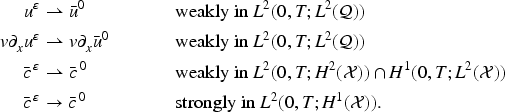
Due to the uniform bounds provided in Theorem 2, a sequence $(u^{\epsilon },{\overline{c}}^{\epsilon })$ of solutions can be extracted which converges to an appropriate limit.

Proposition 11

Under the assumptions of Theorem 2, there exist functions

$${\overline{u}}^0\in L^{\mathrm{\infty }}(0,T;H^1(\mathcal{X}))\text{and}{\overline{c}}^0\in L^2(0,T;H^2(\mathcal{X}))\cap H^1(0,T;L^2(\mathcal{X}))$$

and a sequence $(u^{\epsilon },{\overline{c}}^{\epsilon }{)}_{\epsilon >0}$ of solutions to (2) to (5) such that with $\epsilon \to 0$ one has

$$\begin{array}{rlrl}{u}^{\epsilon }& \rightharpoonup {\overline{u}}^0& & \text{weakly in}{L}^2(0,T;L^2(\mathcal{Q}))\\ v{\mathrm{\partial }}_x{u}^{\epsilon }& \rightharpoonup v{\mathrm{\partial }}_x{\overline{u}}^0& & \text{weakly in}{L}^2(0,T;L^2(\mathcal{Q}))\\ {\overline{c}}^{\epsilon }& \rightharpoonup {\overline{c}}^0& & \text{weakly in}{L}^2(0,T;H^2(\mathcal{X}))\cap H^1(0,T;L^2(\mathcal{X}))\\ {\overline{c}}^{\epsilon }& \to {\overline{c}}^0& & \text{strongly in}{L}^2(0,T;H^1(\mathcal{X})).\end{array}$$

Moreover, the limit function ${\overline{c}}^0$ satisfies the initial and boundary conditions stated in (10).

Proof.

The assertions about ${\overline{c}}^{\epsilon }$ and ${\overline{c}}^0$ follow immediately from the estimates of Theorem 2, the Banach–Alaoglou Theorem (Conway, 2019), the Aubin–Lions compactness lemma (Roubíček, 2013, Lemma 7.7), and the continuity of the trace operators in space and time. By the uniform bounds for $u^{\epsilon }$ , one further obtains a subsequence $u^{\epsilon }$ and a limit $u^0\in L^{\mathrm{\infty }}(0,T;L^2(\mathcal{Q}))$ such that $u^{\epsilon }\rightharpoonup u^0$ and $v{\mathrm{\partial }}_x{u}^{\epsilon }\rightharpoonup v{\mathrm{\partial }}_x{u}^0$ weakly in $L^2(0,T;L^2(\mathcal{Q}))$ . From the weak lower-semicontinuity of norms and the estimates of Theorem 2, it can further be deduced that

$$\Vert u^0-{\overline{u}}^0{\Vert }_{L^2(0,T;L^2(\mathcal{Q}))}\le \underset{\epsilon \to 0}{lim inf}\Vert u^{\epsilon }-{\overline{u}}^{\epsilon }{\Vert }_{L^2(0,T;L^2(\mathcal{Q}))}=0,$$

which implies $u^0={\overline{u}}^0\in L^2(0,T;L^2(\mathcal{X}))$ . Uniqueness of the weak limit shows that $v{\mathrm{\partial }}_x{u}^0=v{\mathrm{\partial }}_x{\overline{u}}^0\in L^2(0,T;L^2(\mathcal{Q}))$ which implies $u^0={\overline{u}}^0\in L^2(0,T;H^1(\mathcal{X}))$ .

As part of the analysis in the next subsection, it will be shown that the limit ${\overline{u}}^0$ also has a weak time derivative and satisfies the initial and boundary conditions (9).

4.3. Further Properties of the Limiting Functions

To conclude the proof of the first part of Theorem 3, it remains to show that the limit functions $({\overline{u}}^0,{\overline{c}}^0)$ provided by Proposition 11 are indeed a weak solution to the Keller–Segel system (6) to (10).

Step 1. From the linearity of the Equations (3) and (7), and the assertions of Proposition 11, one can immediately deduce that $({\overline{u}}^0,{\overline{c}}^0)$ satisfies (7) and (10).

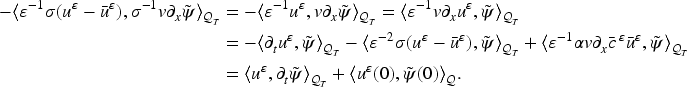
Step 2. The following auxiliary result is needed for the analysis of the kinetic equation. Let $\tilde{\psi }\in C^{\mathrm{\infty }}([0,T];H_0^1(\mathcal{X}))$ with $\tilde{\psi }(T)=0$ be given. Then, from (2) and (4),

$$⟨v{\mathrm{\partial }}_x{u}^{\epsilon },{\sigma }^{-1}v{\mathrm{\partial }}_x\tilde{\psi }{⟩}_{{\mathcal{Q}}_T}=⟨\epsilon u^{\epsilon },{\sigma }^{-1}v{\mathrm{\partial }}_{tx}\tilde{\psi }{⟩}_{{\mathcal{Q}}_T}+⟨\alpha v{\mathrm{\partial }}_x{\overline{c}}^{\epsilon }{\overline{u}}^{\epsilon }-{\epsilon }^{-1}\sigma (u^{\epsilon }-{\overline{u}}^{\epsilon }),{\sigma }^{-1}v{\mathrm{\partial }}_x\tilde{\psi }{⟩}_{{\mathcal{Q}}_T}.$$

For abbreviation the notation ${\mathcal{Q}}_T=\mathcal{Q}\times (0,T)$ and ${\mathcal{X}}_T=\mathcal{X}\times (0,T)$ is used in the following. By the uniform bounds for $u^{\epsilon }$ , one sees that $⟨\epsilon u^{\epsilon },{\sigma }^{-1}v{\mathrm{\partial }}_{tx}\tilde{\psi }{⟩}_{{\mathcal{Q}}_T}\to 0$ with $\epsilon \to 0$ . The first part in the last integral can be split into

$$⟨\alpha v{\mathrm{\partial }}_x{\overline{c}}^{\epsilon }{\overline{u}}^{\epsilon },{\sigma }^{-1}v{\mathrm{\partial }}_x\tilde{\psi }{⟩}_{{\mathcal{Q}}_T}=⟨\alpha v{\mathrm{\partial }}_x{\overline{c}}^0{\overline{u}}^{\epsilon },{\sigma }^{-1}v{\mathrm{\partial }}_x\tilde{\psi }{⟩}_{{\mathcal{Q}}_T}+⟨\alpha v{\mathrm{\partial }}_x({\overline{c}}^{\epsilon }-{\overline{c}}^0){\overline{u}}^{\epsilon },{\sigma }^{-1}v{\mathrm{\partial }}_x\tilde{\psi }{⟩}_{{\mathcal{Q}}_T}.$$

The first term on the right-hand side converges to $⟨\alpha v{\mathrm{\partial }}_x{\overline{c}}^0{\overline{u}}^0,{\sigma }^{-1}v{\mathrm{\partial }}_x\tilde{\psi }{⟩}_{{\mathcal{Q}}_T}$ . Since ${\overline{c}}^{\epsilon }\to {\overline{c}}^0$ strongly in $L^2(0,T;H^1(\mathcal{X}))$ , the last term converges to zero with $\epsilon \to 0$ . Using (1) and (2), the remaining term in the identity above can be rewritten as

$$\begin{array}{rl}-⟨{\epsilon }^{-1}\sigma (u^{\epsilon }-{\overline{u}}^{\epsilon }),{\sigma }^{-1}v{\mathrm{\partial }}_x\tilde{\psi }{⟩}_{{\mathcal{Q}}_T}& =-⟨{\epsilon }^{-1}{u}^{\epsilon },v{\mathrm{\partial }}_x\tilde{\psi }{⟩}_{{\mathcal{Q}}_T}=⟨{\epsilon }^{-1}v{\mathrm{\partial }}_x{u}^{\epsilon },\tilde{\psi }{⟩}_{{\mathcal{Q}}_T}\\ & =-⟨{\mathrm{\partial }}_t{u}^{\epsilon },\tilde{\psi }{⟩}_{{\mathcal{Q}}_T}-⟨{\epsilon }^{-2}\sigma (u^{\epsilon }-{\overline{u}}^{\epsilon }),\tilde{\psi }{⟩}_{{\mathcal{Q}}_T}+⟨{\epsilon }^{-1}\alpha v{\mathrm{\partial }}_x{\overline{c}}^{\epsilon }{\overline{u}}^{\epsilon },\tilde{\psi }{⟩}_{{\mathcal{Q}}_T}\\ & =⟨u^{\epsilon },{\mathrm{\partial }}_t\tilde{\psi }{⟩}_{{\mathcal{Q}}_T}+⟨u^{\epsilon }(0),\tilde{\psi }(0){⟩}_{\mathcal{Q}}.\end{array}$$

By combination of these results and those of Proposition 11, one concludes that

$$\begin{array}{rl}⟨v{\mathrm{\partial }}_x{\overline{u}}^0,{\sigma }^{-1}v{\mathrm{\partial }}_x\tilde{\psi }{⟩}_{{\mathcal{Q}}_T}& =\underset{\epsilon \to 0}{lim}⟨v{\mathrm{\partial }}_x{u}^{\epsilon },{\sigma }^{-1}v{\mathrm{\partial }}_x\tilde{\psi }{⟩}_{{\mathcal{Q}}_T}\\ & =⟨\alpha v{\mathrm{\partial }}_x{\overline{c}}^0{\overline{u}}^0,{\sigma }^{-1}v{\mathrm{\partial }}_x\tilde{\psi }{⟩}_{{\mathcal{Q}}_T}+⟨{\overline{u}}^0,{\mathrm{\partial }}_t\tilde{\psi }{⟩}_{{\mathcal{Q}}_T}+⟨{\overline{u}}_0,\tilde{\psi }(0){⟩}_{\mathcal{Q}}.\end{array}$$

Step 3. By definition of $\overline{\chi }$ and $\overline{\mu }$ in (8), the previous results, further yield that

$$\begin{array}{rl}2⟨\overline{\mu }{\mathrm{\partial }}_x{\overline{u}}^0,{\mathrm{\partial }}_x\tilde{\psi }{⟩}_{{\mathcal{X}}_T}& =⟨v{\mathrm{\partial }}_x{\overline{u}}^0,{\sigma }^{-1}v{\mathrm{\partial }}_x\tilde{\psi }{⟩}_{{\mathcal{Q}}_T}\\ & =2⟨\overline{\chi }{\mathrm{\partial }}_x{\overline{c}}^0{\overline{u}}^0,{\mathrm{\partial }}_x\tilde{\psi }{⟩}_{{\mathcal{X}}_T}+2⟨{\overline{u}}^0,{\mathrm{\partial }}_t\tilde{\psi }{⟩}_{{\mathcal{X}}_T}+2⟨{\overline{u}}_0,\tilde{\psi }(0){⟩}_{\mathcal{X}}.\end{array}$$

This shows that the limit $({\overline{u}}^0,{\overline{c}}^0)$ provided by Proposition 11 satisfies (26). In particular, the distributional time derivative ${\mathrm{\partial }}_t{\overline{u}}^0$ satisfies

$$⟨{\mathrm{\partial }}_t{\overline{u}}^0,\tilde{\psi }⟩:=-⟨{\overline{u}}^0,{\mathrm{\partial }}_t\tilde{\psi }{⟩}_{{\mathcal{X}}_T}=-⟨\overline{\mu }{\mathrm{\partial }}_x{\overline{u}}^0-\overline{\chi }{\mathrm{\partial }}_x{\overline{c}}^0{\overline{u}}^0,{\mathrm{\partial }}_x\tilde{\psi }{⟩}_{{\mathcal{X}}_T}$$

for all $\tilde{\psi }\in C_0^{\mathrm{\infty }}((0,T);H_0^1(\mathcal{X}))$ . From the regularity of ${\overline{u}}^0$ and ${\overline{c}}^0$ , it can be infered that

$$\overline{\mu }{\mathrm{\partial }}_x{\overline{u}}^0-\overline{\chi }{\mathrm{\partial }}_x{\overline{c}}^0{\overline{u}}^0\in L^2(0,T;L^2(\mathcal{X})).$$

This shows that ${\mathrm{\partial }}_t{\overline{u}}^0$ belongs to $L^2(0,T;H^{-1}(\mathcal{X}))$ and, hence, is a weak derivative. Moreover, the variational identity (25) holds for a.a. $t\in (0,T)$ .

Step 4. By combination of (25) and (26), one can immediately see that ${\overline{u}}^0(0)={\overline{u}}_0$ . Now let $\mathrm{tr}:u\mapsto u{|}_{\mathrm{\Gamma }}$ denote the trace operator for $u\in U=\{v\in L^2(\mathcal{Q}):v{\mathrm{\partial }}_{x}u\in L^2(\mathcal{Q})\}$ . By use of the integration-by-parts formula (1), one obtains

$$\Vert \mathrm{tr}u{\Vert }_{L^2(\mathrm{\Gamma };|v|\mathrm{d}\mathrm{\Gamma })}^2={\int }_{\mathrm{\Gamma }}|\mathrm{tr}u{|}^2|v|\mathrm{d}\mathrm{\Gamma }=2{\int }_{\mathcal{Q}}v{\mathrm{\partial }}_{x}uu\mathrm{d}(x,v)\le 2\Vert v{\mathrm{\partial }}_{x}u{\Vert }_{L^2(\mathcal{Q})}\Vert u{\Vert }_{L^2(\mathcal{Q})}.$$

(27)

This shows that the trace operator $\mathrm{tr}:L^2(0,T;U)\to L^2(0,T;L^2(\mathrm{\Gamma };|v|\mathrm{d}\mathrm{\Gamma }))$ is continuous as a mapping between these spaces. Proposition 11 suggests that ${\overline{u}}^{\epsilon }\rightharpoonup {\overline{u}}^0$ weakly in $L^2(0,T;U)$ , and hence $\mathrm{tr}{u}^{\epsilon }\rightharpoonup \mathrm{tr}{\overline{u}}^0$ weakly in $L^2(0,T;L^2(\mathrm{\Gamma };|v|\mathrm{d}\mathrm{\Gamma }))$ . Since $\mathrm{tr}{u}^{\epsilon }={\overline{g}}_u$ on ${\mathrm{\Gamma }}^{in}\times (0,T)$ , it can be inferred that $\mathrm{tr}{\overline{u}}^0={\overline{g}}_u$ on ${\mathrm{\Gamma }}^{in}\times (0,T)$ , and since ${\overline{u}}^0$ is independent of $v$ , one further concludes that ${\overline{u}}^0={\overline{g}}_u$ on $\mathrm{\partial }\mathcal{X}\times (0,T)$ in a trace sense. In summary, it was thus shown that ${\overline{u}}^0$ satisfies the initial and boundary conditions (9), and hence $({\overline{u}}^0,{\overline{c}}^0)$ is a weak solution of (6) to (10).

Step 5. Since every sequence of solutions $(u^{\epsilon },{\overline{c}}^{\epsilon })$ to (2) to (5) for $\epsilon \to 0$ has a subsequence which converges weakly to a weak solution $({\overline{u}}^0,{\overline{c}}^0)$ of (6) to (10) and since the weak solution to this problem is unique according to Proposition 9, this establishes weak convergence with $\epsilon \to 0$ for any sequence $(u^{\epsilon },{\overline{c}}^{\epsilon })$ of solutions. This concludes the first part of the proof of Theorem 3.

5. Proof of Theorem 3, Part 2

In this section, the quantitative convergence rates announced in Theorem 3 are established. Following standard arguments (Dautray & Lions, 1993; Egger & Schlottbom, 2014), the solutions $(u^{\epsilon },{\overline{c}}^{\epsilon })$ are decomposed as

$$\begin{array}{rl}{u}^{\epsilon }& ={\overline{u}}^0+\epsilon v{\overline{u}}^1+{\varphi }^{\epsilon }\text{with}{\overline{u}}^1=-{\sigma }^{-1}{\mathrm{\partial }}_x{\overline{u}}^0+\alpha {\sigma }^{-1}{\mathrm{\partial }}_x{\overline{c}}^0{\overline{u}}^0,\end{array}$$

(28)

$$\begin{array}{rl}{\overline{c}}^{\epsilon }& ={\overline{c}}^0+{\overline{\eta }}^{\epsilon }.\end{array}$$

(29)

Estimates on ${\overline{u}}^1$ and the two remainder terms ${\varphi }^{\epsilon }$ and ${\overline{\eta }}^{\epsilon }$ are established in the sequel to conclude the proof of the theorem.

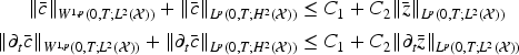
Step 1. From the regularity of the limit solution $({\overline{u}}^0,{\overline{c}}^0)$ provided by Proposition 9, it can be deduced that $\Vert {\overline{u}}^1{\Vert }_{L^{\mathrm{\infty }}(0,T;L^{\mathrm{\infty }}(\mathcal{X}))}$ , $\Vert {\mathrm{\partial }}_x{\overline{u}}^1{\Vert }_{L^2(0,T;L^2(\mathcal{X}))}$ , and $\Vert {\mathrm{\partial }}_t{\overline{u}}^1{\Vert }_{L^2(0,T;L^2(\mathcal{X}))}$ are uniformly bounded. In addition, one has

$$\overline{v{\overline{u}}^1}=0,\text{ and consequently}{\overline{\varphi }}^{\epsilon }={\overline{u}}^{\epsilon }-{\overline{u}}^0.$$

(30)

As a consequence, some of the terms in the following investigations will vanish.

Step 2. Using the equations defining ${\overline{c}}^{\epsilon }$ and ${\overline{c}}^0$ , one sees that ${\overline{\eta }}^{\epsilon }={\overline{c}}^{\epsilon }-{\overline{c}}^0$ satisfies

$${\mathrm{\partial }}_t{\overline{\eta }}^{\epsilon }-D{\mathrm{\partial }}_{xx}{\overline{\eta }}^{\epsilon }+\beta {\overline{\eta }}^{\epsilon }=\gamma {\overline{\varphi }}^{\epsilon }\text{in }\mathcal{X}\times (0,T),$$

(31)

together with homogeneous initial and boundary conditions. From standard a priori estimates for parabolic equations (Evans, 2010), one thus obtains

$$\Vert {\overline{\eta }}^{\epsilon }{\Vert }_{L^{\mathrm{\infty }}(0,T;L^2(\mathcal{X}))}\le \Vert {\overline{\eta }}^{\epsilon }{\Vert }_{L^{\mathrm{\infty }}(0,T;H^1(\mathcal{X}))}+\Vert {\overline{\eta }}^{\epsilon }{\Vert }_{L^2(0,T;H^2(\mathcal{X}))}\le C\Vert {\varphi }^{\epsilon }{\Vert }_{L^2(0,T;L^2(\mathcal{Q}))}.$$

It therefore remains to establish the appropriate bounds for the second remainder ${\varphi }^{\epsilon }$ .

Step 3. From the equations defining $u^{\epsilon }$ , ${\overline{u}}^0$ , and ${\overline{u}}^1$ , one sees that ${\varphi }^{\epsilon }$ solves

$$\begin{array}{rlrl}{\epsilon }^2{\mathrm{\partial }}_t{\varphi }^{\epsilon }+\epsilon v{\mathrm{\partial }}_x{\varphi }^{\epsilon }+\sigma ({\varphi }^{\epsilon }-{\overline{\varphi }}^{\epsilon })& =\epsilon f^{\epsilon }& & \text{in }\mathcal{Q}\times (0,T),\end{array}$$

(32)

$$\begin{array}{rlrl}{\varphi }^{\epsilon }& =g^{\epsilon }& & \text{on }{\mathrm{\Gamma }}^{\mathrm{in}}\times (0,T),\end{array}$$

(33)

$$\begin{array}{rlrl}{\varphi }^{\epsilon }(0)& ={\varphi }_0^{\epsilon }& & \text{on }\mathcal{Q}\end{array}$$

(34)

with $f^{\epsilon }=\alpha v{\mathrm{\partial }}_x{\overline{c}}^{\epsilon }{\overline{u}}^{\epsilon }-\epsilon {\mathrm{\partial }}_t{\overline{u}}^0-v{\mathrm{\partial }}_x{\overline{u}}^0-{\epsilon }^{2}v{\mathrm{\partial }}_t{\overline{u}}^1-\epsilon v^2{\mathrm{\partial }}_x{\overline{u}}^1-\sigma v{\overline{u}}^1$ , $g^{\epsilon }=-\epsilon v{\overline{u}}^1$ , and initial value ${\varphi }_0^{\epsilon }=-\epsilon v{\overline{u}}^1(0)$ . Following the arguments in Egger and Schlottbom (2014), a split ${\varphi }^{\epsilon }={\varphi }_f^{\epsilon }+{\varphi }_g^{\epsilon }$ is conducted with ${\varphi }_f^{\epsilon }$ solving the same system, but with homogeneous boundary conditions, and ${\varphi }_g^{\epsilon }$ satisfying the equations with homogeneous right hand side and homogeneous initial conditions.

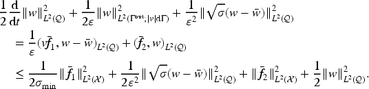
Step 3a. As a preliminary result, $L^p$ bounds for ${\varphi }_g^{\epsilon }$ are established, elaborating explicitly on the dependence on $\epsilon$ . To do so, multiply (32) with $f^{\epsilon }=0$ by $|{\varphi }_g^{\epsilon }{|}^{p-2}{\varphi }_g^{\epsilon }$ , which yields

$${\epsilon }^2\frac{1}{p}{\mathrm{\partial }}_t|{\varphi }_g^{\epsilon }{|}^p+\epsilon v\frac{1}{p}{\mathrm{\partial }}_x|{\varphi }_g^{\epsilon }{|}^p=\sigma ({\overline{\varphi }}_g^{\epsilon }-{\varphi }_g^{\epsilon })|{\varphi }_g^{\epsilon }{|}^{p-2}{\varphi }_g^{\epsilon }.$$

Integration over $\mathcal{Q}\times (0,t)$ , application of the integration-by-parts formula (1), and of the inhomogeneous boundary and homogeneous initial conditions for ${\varphi }_g^{\epsilon }$ yields

$$\begin{array}{rl}& \frac{{\epsilon }^2}{p}\Vert {\varphi }_g^{\epsilon }(t){\Vert }_{L^p(\mathcal{Q})}^p+{\int }_0^t{\int }_{{\mathrm{\Gamma }}^{\mathrm{out}}}\frac{\epsilon }{p}|v||{\varphi }_g^{\epsilon }{|}^p\mathrm{d}\mathrm{\Gamma }\mathrm{d}s\end{array}$$

(35)

$$\begin{array}{rl}& ={\int }_0^t{\int }_{{\mathrm{\Gamma }}^{\mathrm{in}}}\frac{\epsilon }{p}|v||\epsilon v{\overline{u}}^1{|}^p\mathrm{d}\mathrm{\Gamma }\mathrm{d}s+{\int }_0^t{\int }_{\mathcal{Q}}\sigma ({\overline{\varphi }}_g^{\epsilon }-{\varphi }_g^{\epsilon })|{\varphi }_g^{\epsilon }{|}^{p-2}{\varphi }_g^{\epsilon }d(x,v)\mathrm{d}s.\end{array}$$

By Hölder’s inequality, one sees that

$${\int }_{\mathcal{V}}\overline{u}|u{|}^{p-2}u\mathrm{d}v\le {\left({\int }_{\mathcal{V}}|\overline{u}{|}^p\mathrm{d}v\right)}^{1/p}{({\int }_{\mathcal{V}}(|u{|}^{p-1}{)}^{\frac{p}{p-1}}\mathrm{d}v)}^{(p-1)/p}$$

for any $u\in L^p(\mathcal{V})$ , and Jensen’s inequality further yields $({\int }_{\mathcal{V}}|\overline{u}{|}^p\mathrm{d}v{)}^{1/p}\le ({\int }_{\mathcal{V}}|u{|}^p\mathrm{d}v{)}^{1/p}$ for any $p\ge 2$ . By combination of these estimates, one concludes that the last term in the second line of (35) is non-positive. Since $|v|\le 1$ , the inequality then simplifies to

$$\Vert {\varphi }_g^{\epsilon }(t){\Vert }_{L^p(\mathcal{Q})}\le {\epsilon }^{-1/p}{\left({\int }_0^t{\int }_{{\mathrm{\Gamma }}^{in}}|\epsilon {\overline{u}}^1{|}^p\mathrm{d}\mathrm{\Gamma }\mathrm{d}s\right)}^{1/p}\le C{\epsilon }^{1-1/p}.$$

For the last step, the trace theorem and the uniform boundedness of ${\overline{u}}^1$ according to Step 1 were used. By letting $p\to \mathrm{\infty }$ , one obtains

$$\Vert {\varphi }_g^{\epsilon }{\Vert }_{L^{\mathrm{\infty }}(0,T;L^{\mathrm{\infty }}(\mathcal{Q}))}=\underset{p\to \mathrm{\infty }}{lim}\Vert {\varphi }_g^{\epsilon }{\Vert }_{L^{\mathrm{\infty }}(0,T;L^p(\mathcal{Q}))}\le C^{\prime }\epsilon .$$

(36)

Since $\mathcal{X}$ is bounded, one further has $\Vert {\varphi }_g^{\epsilon }{\Vert }_{L^{\mathrm{\infty }}(0,T;L^2(\mathcal{Q}))}\le C\Vert {\varphi }_g^{\epsilon }{\Vert }_{L^{\mathrm{\infty }}(0,T;L^{\mathrm{\infty }}(\mathcal{Q}))}\le C^{″}\epsilon$ , which is the desired bound for the first component of ${\varphi }^{\epsilon }$ .

Step 3b. The rate for ${\varphi }_f^{\epsilon }$ is based on a bound on the right hand side of (32). The definition of ${\overline{u}}^1$ shows that $\sigma {\overline{u}}^1=\alpha {\mathrm{\partial }}_x{\overline{c}}^0{\overline{u}}^0-{\mathrm{\partial }}_x{\overline{u}}^0$ . Further using (7), one can rewrite

$$f^{\epsilon }=\alpha v({\mathrm{\partial }}_x{\overline{c}}^{\epsilon }{\overline{u}}^{\epsilon }-{\mathrm{\partial }}_x{\overline{c}}^0{\overline{u}}^0)-{\epsilon }^{2}v{\mathrm{\partial }}_t{\overline{u}}^1-\epsilon [v^2{\mathrm{\partial }}_x{\overline{u}}^1+{\mathrm{\partial }}_x(\overline{\mu }{\mathrm{\partial }}_x{\overline{u}}^0-\overline{\chi }{\mathrm{\partial }}_x{\overline{c}}^0{\overline{u}}^0)].$$

(37)

Using the formula (8) defining $\overline{\mu }$ , $\overline{\chi }$ , and ${\overline{u}}^1$ , one sees that

$${\int }_{\mathcal{V}}(v^2{\mathrm{\partial }}_x{\overline{u}}^1+{\mathrm{\partial }}_x(\overline{\mu }{\mathrm{\partial }}_x{\overline{u}}^0-\overline{\chi }{\mathrm{\partial }}_x{\overline{c}}^0{\overline{u}}^0))\mathrm{d}v=0,$$

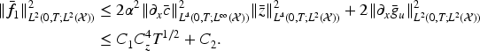
and hence ${\overline{f}}^{\epsilon }=0$ . Noting that the function $f^{\epsilon }$ can be treated like the term $v{\overline{f}}_1$ in the system (16) and (17), the energy estimate (21) thus gives

$$\Vert {\varphi }_f^{\epsilon }{\Vert }_{L^{\mathrm{\infty }}(0,t;L^2(\mathcal{Q}))}^2\le e^t(\Vert {\varphi }_f^{\epsilon }(0){\Vert }_{L^2(\mathcal{Q})}^2+\Vert f^{\epsilon }{\Vert }_{L^2(0,t;L^2(\mathcal{Q}))}^2)$$

for any $0\le t\le T$ . From the bounds for ${\overline{u}}_1$ , one obtains $\Vert {\varphi }_f^{\epsilon }(0){\Vert }_{L^2(\mathcal{Q})}^2\le C_0{\epsilon }^2$ . The right hand side (37) may be split into $f^{\epsilon }=f_0^{\epsilon }+\epsilon f_1^{\epsilon }+{\epsilon }^2{f}_2^{\epsilon }$ . From the bounds for ${\overline{u}}^0$ and ${\overline{u}}^1$ , one immediately obtains that $\Vert \epsilon f_1^{\epsilon }+{\epsilon }^2{f}_2^{\epsilon }{\Vert }_{L^2(0,T;L^2(\mathcal{Q}))}\le C\epsilon$ . Using Hölder and triangle inequalities, the remaining term can be estimated as follows

$$\begin{array}{rl}\Vert f_0^{\epsilon }{\Vert }_{L^2(L^2)}& \le \alpha \Vert {\mathrm{\partial }}_x{\overline{c}}^{\epsilon }{\overline{u}}^{\epsilon }-{\mathrm{\partial }}_x{\overline{c}}^0{\overline{u}}^0{\Vert }_{L^2(L^2)}\\ & \le \alpha (\Vert {\mathrm{\partial }}_x{\overline{c}}^{\epsilon }-{\mathrm{\partial }}_x{\overline{c}}^0{\Vert }_{L^2(L^{\mathrm{\infty }})}\Vert {\overline{u}}^{\epsilon }{\Vert }_{L^{\mathrm{\infty }}(L^2)}+\Vert {\mathrm{\partial }}_x{\overline{c}}^0{\Vert }_{L^{\mathrm{\infty }}(L^{\mathrm{\infty }})}\Vert {\overline{u}}^{\epsilon }-{\overline{u}}^0{\Vert }_{L^2(L^2)}).\end{array}$$

By previous a priori estimates, one can bound $\Vert {\overline{u}}^{\epsilon }{\Vert }_{L^{\mathrm{\infty }}(L^2)}\le C$ and $\Vert {\mathrm{\partial }}_x{\overline{c}}^0{\Vert }_{L^{\mathrm{\infty }}(L^{\mathrm{\infty }})}\le C$ . Using the equation defining ${\overline{\eta }}^{\epsilon }={\overline{c}}^{\epsilon }-{\overline{c}}^0$ , the definition of ${\varphi }^{\epsilon }$ , and the left identity of (30), the two terms involving differences can be further bounded by

$$\Vert {\mathrm{\partial }}_x{\overline{c}}^{\epsilon }-{\mathrm{\partial }}_x{\overline{c}}^0{\Vert }_{L^2(L^{\mathrm{\infty }})}^2+\Vert {\overline{u}}^{\epsilon }-{\overline{u}}^0{\Vert }_{L^2(L^2)}^2\le C_2\Vert {\varphi }^{\epsilon }{\Vert }_{L^2(L^2)}^2\le C_3(\Vert {\varphi }_f^{\epsilon }{\Vert }_{L^2(L^2)}^2+{\epsilon }^2).$$

In the last step, the bound for $\Vert {\varphi }_g^{\epsilon }{\Vert }_{L^2(L^2)}^2$ from before was used. In summary, one thus gets

$$\Vert f^{\epsilon }{\Vert }_{L^2(0,t;L^2(\mathcal{Q}))}^2\le C_1\Vert {\varphi }_f^{\epsilon }{\Vert }_{L^2(0,t;L^2(\mathcal{Q}))}^2+C_2{\epsilon }^2.$$

Inserting this into the energy estimate for ${\varphi }_f^{\epsilon }$ and applying a Grönwall inequality then leads to the uniform bound $\Vert {\varphi }_f^{\epsilon }{\Vert }_{L^{\mathrm{\infty }}(0,T;L^2(\mathcal{Q}))}^2\le C_2^{\prime }{\epsilon }^2$ .

Step 3c. A combination of the previous estimates shows that

$$\Vert {\varphi }^{\epsilon }{\Vert }_{L^{\mathrm{\infty }}(L^2)}\le \Vert {\varphi }_f^{\epsilon }{\Vert }_{L^{\mathrm{\infty }}(L^2)}+\Vert {\varphi }_g^{\epsilon }{\Vert }_{L^{\mathrm{\infty }}(L^2)}\le C\epsilon .$$

From the definition of ${\varphi }^{\epsilon }$ and the uniform bounds for ${\overline{u}}^1$ , one then gets

$$\Vert u^{\epsilon }-{\overline{u}}^0{\Vert }_{L^{\mathrm{\infty }}(0,T;L^2(\mathcal{Q}))}\le \epsilon \Vert v{\overline{u}}^1{\Vert }_{L^{\mathrm{\infty }}(0,T;L^2(\mathcal{Q}))}+\Vert {\varphi }^{\epsilon }{\Vert }_{L^{\mathrm{\infty }}(0,T;L^2(\mathcal{Q}))}\le C\epsilon .$$

From the arguments of Step 2, one concludes that $\Vert {\overline{c}}^{\epsilon }-{\overline{c}}^0{\Vert }_{L^{\mathrm{\infty }}(0,T;L^2(\mathcal{Q}))}\le C\epsilon$ as well, which proves the convergence rates stated in Theorem 3.

6. Discussion and Possible Extensions

This articles establishes well-posedness of a kinetic chemotaxis model in slab geometry and convergence to a drift–diffusion system of Keller–Segel type in the asymptotic limit. The results are valid on a finite time interval $[0,T]$ with $T>0$ depending on the problem data. As mentioned in Remark 4, the results can be extended to $T=\mathrm{\infty }$ if flux limiting is used in the chemotaxis term. We expect the global in time results to remain valid also without flux limiting, which however requires a different analysis. The results in this work can be extended quite naturally to related chemotaxis models on networks which were introduced as mathematical models for dermal wound healing (Bretti et al., 2014) or the growth of slime molds (Borsche et al., 2014). The fact that the velocity space $\mathcal{V}=(-1,1)$ involves a whole interval here means that agents can actually move at different speeds. Such systems have been studied numerically in Borsche et al. (2016). The asymptotic analysis for somewhat simplified coupling conditions has been derived (Philippi, 2023), and corresponding results for the limiting Keller–Segel model on networks were obtained in Borsche et al. (2014); Egger and Schöbel-Kröhn (2020).

Possible topics for future research include the extension of the results derived in this paper to more complex interaction mechanisms, involving multiple species, different chemo-attractants, or more complex coupling mechanisms; see Bitsouni and Eftimie (2018); Emako et al. (2015); Ren and Liu (2020) for some recent work in this direction. The design of asymptotic preserving numerical schemes for chemotaxis in slab geometry and related models on networks, in a similar spirit to Carrillo and Yan (2013); Gosse (2013); Natalini and Ribot (2012), would be a topic for future research.