
Abstract
In order to prove classical planning instances unsolvable, state-of-the-art planners resort to a state space search. However, we show here that an incomplete, yet computationally efficient criterion is sometimes sufficient to immediately identify as unsolvable a wide range of planning instances. Based on linear and integer programming, we show in this paper how it can be leveraged, should it fail at first. This criterion is the keystone of various techniques we propose to rewrite and enhance the STRIPS model, so as to gather new information about it. If the newly found bits of information is not sufficient to identify the instance as unsolvable, they still constitute human-readable bits of information that can provide additional insight on the planning instance.
Introduction
Current classical planners go through a search phase, with the aim of finding a sequence of actions that satisfies a given goal. They often start with the assumption that such a plan exists, and for the past few decades, significant work has been done on designing more and more efficient techniques to find solution plans. However, various reasons may lead to an instance not admitting any solution. Search-based planners will then explore the state space in its entirety, potentially cutting branches of the search tree, until they realize no plan can be found. The detection of states that cannot lead to any solution is often a byproduct of the heuristics used during search: an infinite heuristic value for an admissible heuristic is a synonym of a dead-end state.
This is why in recent years, there has been a renewed interest in detecting unsolvable planning instances, as illustrated by the 2016 Unsolvability International Planning Competition (Unsolvability IPC). Various techniques have been developed in the last couple of decades, such as dead-end formulas (Cserna et al., 2018) and traps (Lipovetzky et al., 2016; Steinmetz et al., 2022). However, all of these methods are based on the exploration of the state space.
In this article, we propose to leverage a linear programming (LP)- and integer programming (IP)-based criterion to iteratively refine a planning model, to show its unsolvability. The criterion we use is fast to compute and allows us to quickly recognize a wide range of unsolvable planning instances. However, it is not complete, in the sense that it may not recognize some unsolvable instances as such. Nevertheless, we show how to use it to iteratively refine the planning model, and keep gathering additional information about the instance with the aim that our procedure can detect that it is unsolvable.
Most of our techniques to gather information are based on a simple schema: after testing the solvability of planning instances
More generally, being able to detect planning instances that have no solution can have various applications in itself. For instance, consider the case where an instance models the attacks that a malicious user may perform on a system, with the goal of accessing restricted data. Finding that no sequence of actions may achieve this shows that the system is secure.
The paper is organized as follows. In Section 2, we introduce our formalism and notations for classical planning. In Section 3, we present the mathematical-programming-based criterion we use throughout this paper. In Section 4, we show how to design tests to gather new information about a planning model. In Section 5, we report our experimental trials on standard sets of benchmarks. Section 6 reviews related work, while Section 7 is devoted to a discussion and perspectives on our findings.
Background
STRIPS Planning Instance
A STRIPS planning instance is a tuple
Note that we define a version of STRIPS with negative goals. The original STRIPS formulation only specified positive goals, and is not any less expressive: any instance with negative goals can be translated, in polynomial time, into an equivalent instance without negative goals. We nonetheless allow negative goals in our formulation of STRIPS, since later in this paper we investigate the possibility of adding negative goals in order to strengthen a STRIPS instance. But one should keep in mind that most planning instances (and in particular, the ones used in our set of benchmarks) come with positive goals only: this is why we assume
Something similar could be said for the preconditions of operators: standard STRIPS only defines positive preconditions, since any STRIPS instance with negative preconditions can be translated into an equivalent instance without negative preconditions in linear time (Geffner & Bonet, 2013). Some versions of STRIPS allow negative preconditions; however, in this case, disallowing negative preconditions makes the formulation of some of our criteria simpler, hence our choice to use this version of STRIPS.
Without loss of generality, we assume that for all operators
States and Plans
A state
Given an instance
Detecting Unsolvable Instances by LP
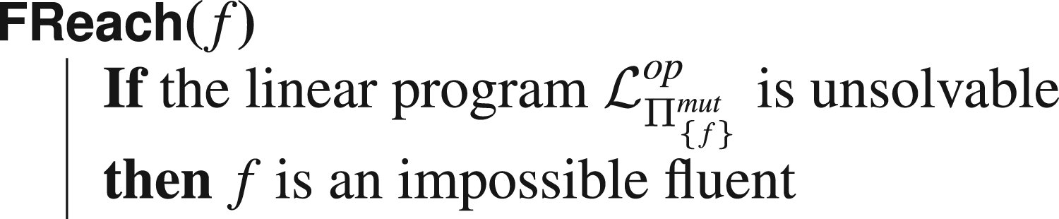
This section introduces two equivalent criteria that we use, and extend, to detect a planning instance’s unsolvability. These criteria are incomplete, in the sense that they cannot detect all unsolvable planning instances by themselves. However, they require very limited computational resources, and are fast to run, as they are based on LP or IP. We will show later how to leverage those properties in order to make the most of these criteria when they are not able to detect an instance’s unsolvability by themselves.
Potential-Based Argument
The first LP formulation that we worked with is based on the following argument. Suppose that we have a numerical function
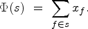
Such a function
More formally, let us consider two sets of operators, with regard to some fluent
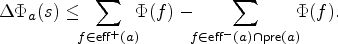
This leads to the following inequality, which models the limit case previously presented. This effectively gives us an upper bound on the change of potential induced by
The only remaining issue is to check whether such a potential function
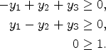
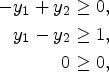
Let


Note that the set of constraints above is not a linear program per se, since it contains the strict inequality (1). However, it can be easily reduced to an actual linear program (for instance by replacing
The following proposition follows from the discussion further above.
Let
Suppose that the hypothesis is true, and let
Note that the converse of Proposition 1 is not true: not all unsolvable planning instances are detected by the criterion we propose.
Our definition of potential is reminiscent of potential heuristics, as introduced by Pommerening et al. (2015): facts are assigned numerical values, also called potentials, which uniquely and compactly define the potentials of all states of the planning instance. In their paper, the authors do so in order to synthesize a heuristic
The main differences with our work lie in two points. First, potential heuristics are defined for planning tasks in Finite Domain Representation (FDR), where variables describing states are not binary, but can have domains of arbitrary size. They are then, in theory, slightly more general than our formulation. Second, while potentials in Pommerening et al. (2015) range over
The linear program presented in the previous section is hard to interpret, as the concept of potential we introduced has no reality outside of the criterion. However, we show in this section how to transform it into another program that can equivalently allow us to detect some unsolvable instances, but whose result is easier to interpret.
To this effect, we resort to Farkas’s lemma. Farkas’s lemma is related to the well-known fact that in LP, the primal problem is feasible iff the dual problem is feasible. One version of this lemma states that exactly one of the following sets of equations has a solution: either (1)
(
)
Let


where
Let
Let

The contrapositive of Lemma 1 is an alternative proof that, if
If
The proof is immediate, as each operator appears an integral number of times in any solution plan
Linear Program 2 is, in fact, an LP formulation of the state equation heuristic (Bonet, 2013), as previously shown in Pommerening et al. (2014). Its efficiency for detecting unsolvable planning instances has been shown before, as it is part of the Aidos planner, which won the Unsat IPC in 2016 (Seipp et al., 2016). The planner uses the LP formulation of the operator-counting heuristic to detect dead ends during search, working on a FDR of the instance. As a consequence, Aidos can detect every instance on which our criterion succeeds: when Linear Program 2 detects some instance
Even though we introduced
Since Linear Program 2 is the dual of Linear Program 1, and both programs can thus be used equivalently, we will only use Linear Program 2 in the rest of this paper. This is motivated by the fact that its formulation is more intuitive, since counting the occurrences of each operator in some plan is more tangible than associating an abstract potential to fluents. This allows us to reinvest Linear Program 2 in a variety of ways our initial formulation could not be reused, as will be shown later.
In the next section, we show that, in the case where the criterion introduced here fails, it can still be leveraged to gather additional information about
This section is dedicated to extending and adding information to the initial planning instance, mainly with the goal of proving it unsolvable. Through various methods, we either add or remove elements from the input model
In the following, we call operation any such method. In the specific case where the operation answers a boolean question (e.g., Is an action removable?), we call it a test.
Note that ultimately, our goal is to detect unsolvable instances as such. As the set of solution plans is empty, its elements and itself satisfy various otherwise uncommon properties. For instance, any operator can be removed without altering the set of solutions. This is why we search for properties on elements of
In the rest of this section, we illustrate the previous general principles through various operations, that allow us to find new information about the planning instance given as input. As our goal is to detect unsolvable instances, in the following, we assume that the criterion could not detect, at first, that the instance is unsolvable and that we have to gather additional information in order to do so. This section concludes with a very simple example showing that, were the criterion to fail at first, it can still be used to prove an instance unsolvable.
Operator Counts and Landmarks
Landmark Detection
An operator
Let
This allows us to define the landmark detection test below, where

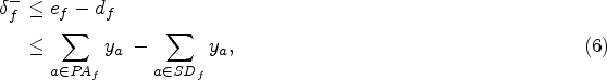
One can generalize the notion of landmark, by counting the least number of times an operator appears in any solution plan. This is why we define the function
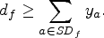
Reasoning on the number of occurrences of some operator
(
)
Let

Let
The proof is a consequence of Lemma 1. We consider only the case where
This gives the following two tests.
In the rest of this paper, we will often use the notation
We use the above tests to maintain estimates of the values of

Operator Mutexes
Operator mutexes are unordered pairs of operators
Finding Operator Mutexes Through LP
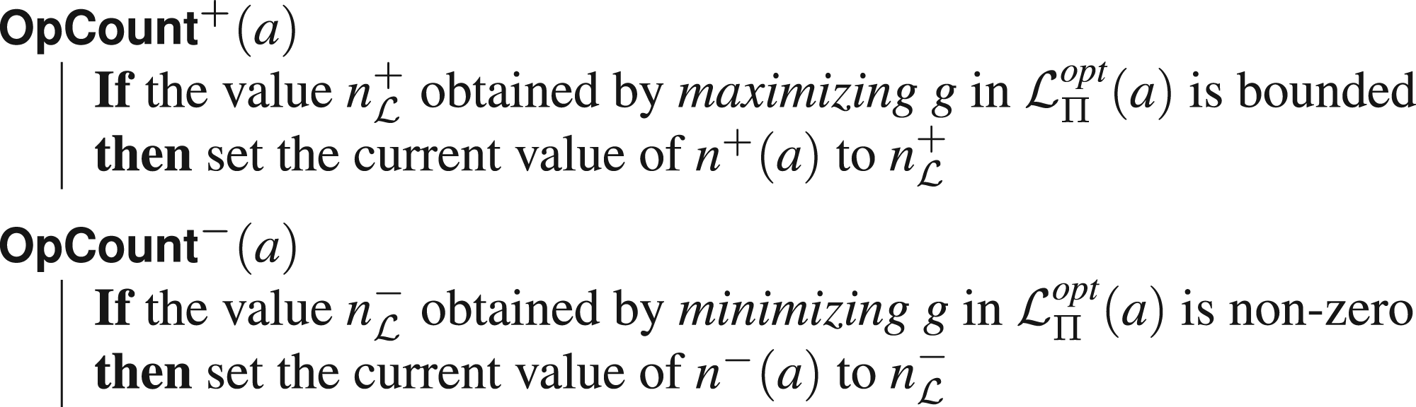
In order to check if two operators


Including the information we have about operator mutexes in the linear program is straightforward. Knowing that
In order to achieve so, we introduce binary variables of the form


This section is concerned with finding operators
Through a Modification of the Linear Program
We start by extending
We do not elaborate on this argument further, as it is a special case of the technique seen in Section 4.1. Indeed, it is equivalent to show that
Unreachable Preconditions
A simple way to prove that some operator
Removing some operators relaxes the linear program

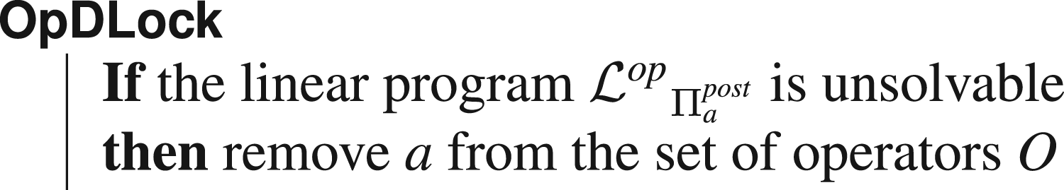
Dead-End Operators
As it is possible to test whether or not there exists a reachable state where
This paragraph is dedicated to finding such operators, called dead-end operators. In order to do so, we need to restrict ourselves to the few fluents that appear in all states resulting from the application of
Let
We prove the contrapositive: suppose that
Then we show in what follows that
Let
We have shown that the initial state of the sequence of states associated with
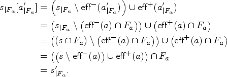
Formally, this can be shown by successively applying the definition of the projection of
Experimental trials showed that no operator could be proved to be a dead-end operator. This is why, in Section 5, no results are reported about the above test. However, we still included this test to show that some very small problems derived from the input instance can be of interest.
In this section, we propose various methods to find more precise goal states. More specifically, we try to add new literals to the goal, be they positive or negative. Suppose, for instance, that some fluent
This can be done in our framework through the following simple observation. Let
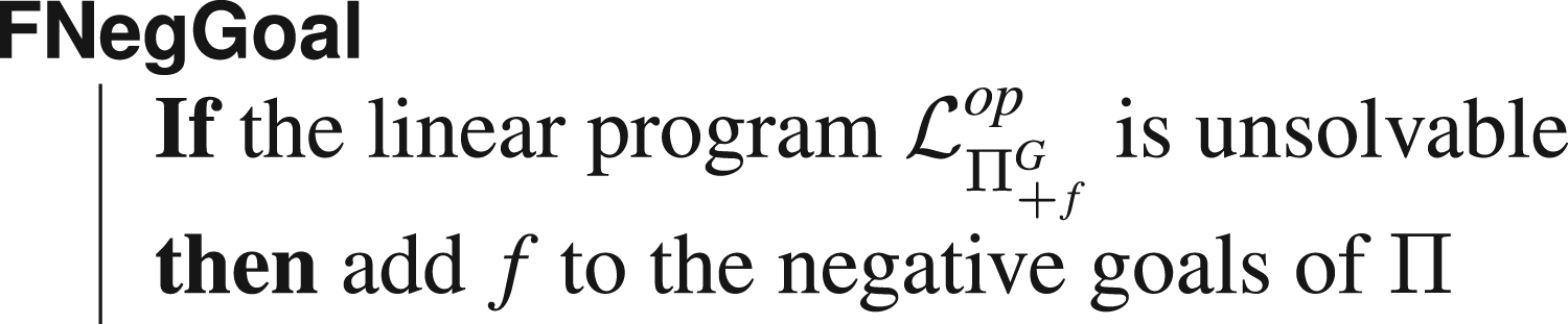
There is, of course, a symmetrically equivalent test
Fluent Mutexes and Unreachable Fluents
A fluent mutex is a set of fluents
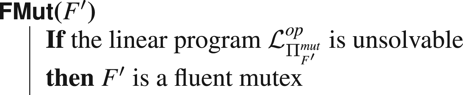
The criterion does not detect all fluent mutexes, and each candidate set of fluents has to be tested individually. Thus, since there exists an exponential number of candidates to test, it is not possible to detect in reasonable time the ones that are within the reach of our method. Finding which sets are interesting to test is a problem in itself; even more so since one has to know how to make use of the newly found information that some
In the general case, we could not find a way to reinvest into the linear program the knowledge that a set of fluents is a mutex. Indeed, Linear Program 2 reasons over the number of times operators (have to) occur in a plan. As a consequence, we do not have any obvious way to reason about properties concerning states, which is precisely what fluent mutexes are. For that reason, we do not include in our routine computation of mutexes through our linear program, even though we can detect a range of fluent mutexes.
However, some fluents are always false, in the sense that no plan will ever establish them. We call the fluents unreachable fluents, and they can be detected with the same argument as above:
Even though these fluents appear very rarely, as will be shown in the experimental trials, it remains linear to test for all fluents whether they are unreachable or not: thus, the computational burden is significantly lower than for other fluent “mutexes.” When an unreachable fluent is detected, one can project the whole instance on fluents
Example Instance Solved Through Model Refinement
In the rest of this section, we show that, when an instance is unsolvable but could not be detected as such by our criterion, then modifying the model using the above operations can still be enough to show the instance unsolvable.
Consider the instance
The associated linear program


The above linear program is solvable (consider for instance the solution where
However, let us apply the test
Note that the above sequence of operations could have been done equivalently with Linear Program 1 instead.
Our implementation was done in Python 3.10, basing ourselves on the Fast Downward parser (Helmert, 2006). We did not need the entire translator component, but only the functions concerned with the conversion of the instance into STRIPS. For linear programs, we resorted to the GLOP solver (Perron & Furnon, 2019), while integer programs were solved with Gurobi (Gurobi Optimization, LLC, 2023). We also used Google ORTools (Perron & Furnon, 2019) to interface between our program and the solvers. We ran our experiments on a machine running Rocky Linux 8.5, powered by an Intel Xeon E5-2667 v3 processor, with a 30-minute cutoff and using at most 16 GB of memory per instance. Our code is available online at https://github.com/arnaudlequen/MPRefinement.
In addition to the evaluation of the linear program, we also implemented a procedure based on the observations of Section 4. The main loop of this procedure consists of executing sequentially a predetermined list of operations and tests, until the instance is detected as unsolvable or the list is depleted. We elaborate further on this in Section 5.2.
We wished to evaluate our program on two different aspects: first, its ability to detect unsolvable instances, and second, its ability to find additional information when it could not conclude.
Our set of benchmarks consists of the unsolvable instances from the unplannability track of the International Planning Competition 2016 (Unsat IPC), for which we report our results on unsolvable instances. The Unsat IPC also includes solvable instances, which we tested our program on, as a sanity check, with success.
LP-Based Criteria
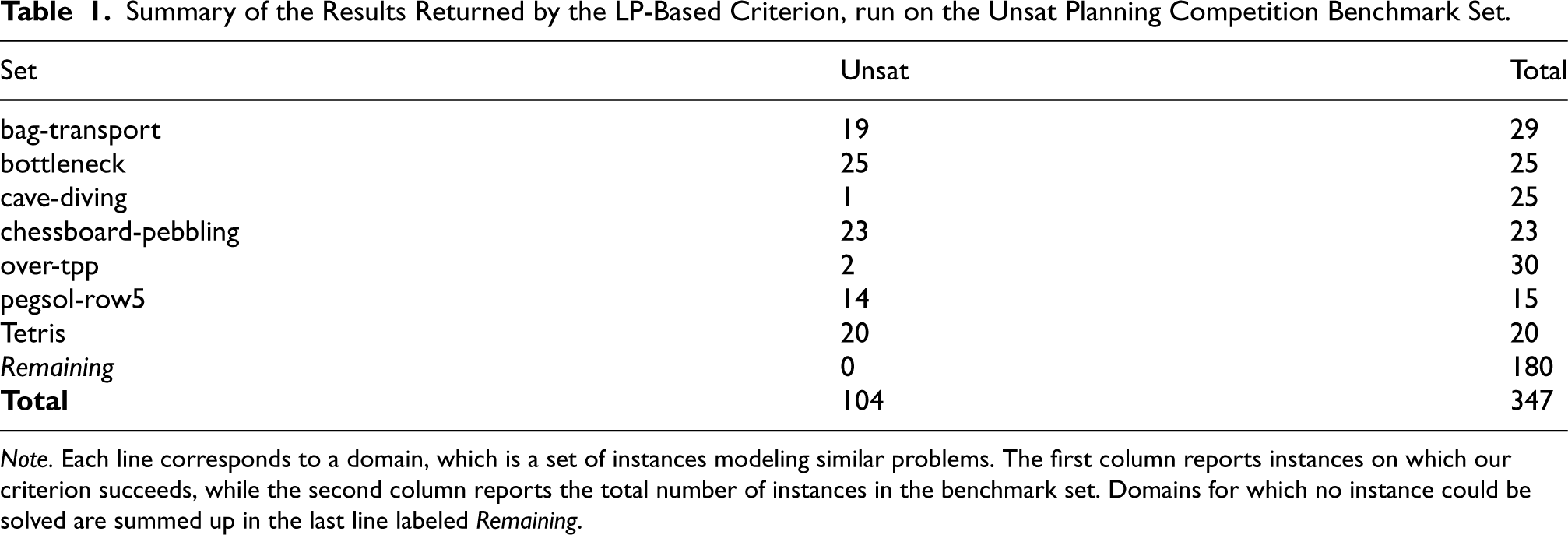
In this section, we show that our LP-based criterion suffices to detect a wide range of unsolvable planning instances. Our results are reported in detail in Table 1.
Summary of the Results Returned by the LP-Based Criterion, run on the Unsat Planning Competition Benchmark Set.
Summary of the Results Returned by the LP-Based Criterion, run on the Unsat Planning Competition Benchmark Set.
Note. Each line corresponds to a domain, which is a set of instances modeling similar problems. The first column reports instances on which our criterion succeeds, while the second column reports the total number of instances in the benchmark set. Domains for which no instance could be solved are summed up in the last line labeled Remaining.
In essence, about 30% of all instances of the Unsat IPC are almost immediately found to be unsolvable by the sole use of the criterion. These results, however, vary greatly from one domain to the other, in a very dichotomous fashion: either the domain is (almost) entirely solved through the criterion, or few to no instances are deemed unsolvable. In the case of domain bag-transport, which seems to be in between, all instances the criterion has been tried on are actually found to be unsolvable: however, as the last 10 instances are too big to be parsed, we could not run the test on them. We can also note that both LP- and IP-based criteria yield the same results and that solving the IP-based program did not allow us to detect more unsolvable instances than through the LP formulation.
Both programs are, however, very lightweight: for most domains, building and solving the program required less than a few seconds. In addition, for the vast majority of instances, the criteria required little more than a few tenths of a second to complete. This further justifies our use of the program in the iterative procedure that we present in the next section.
Our program fails entirely on some domains, where no instance can be solved. While this is often because our criterion simply fails to detect the instance’s unsolvability, this can also be due to the size of the model. This is the case of the bag-gripper, where the first instance has 5,681 fluents and 60,602 operators, which prevents us from building the associated linear program. In our assessments of the performances of the criteria, the limitation always came from memory. In this kind of situation, criteria that work on the FDR of the task might prove more efficient, since for the same problem, 317 facts resulting from 10 variables suffice to describe the first instance of bag-gripper (although 60602 operators are still needed). This may partly explain the success of other FDR-based criteria (Christen et al., 2022; Seipp et al., 2016) in some instances in which our criterion (and thus our procedure) entirely fails because of memory issues.
In the case where the criterion could not immediately detect that an instance
Sequences of Operations
We present below the different lists of operations that we chose. Note that all sequences start and end with a simple test of solvability with the criterion: initially with only the information contained in the STRIPS model, and then with the information that was incrementally gathered after each series of operations. The exact sequences of operations can be found in Appendix A.
Linear
This sequence comprises all tests and operations that are linear in the size of the instance, that is, that only require one argument. We tried to put first the tests that were the most likely to succeed, so that the following tests and operations that come after have more information to work with. We successively apply the following tests on all relevant elements, in that order:
Quadratic
In addition to the tests found in the linear sequence, the quadratic sequence has a sequence of operator mutexes tests
OperatorPreImpossible
As will be reported later, the
OperatorCount
This sequence consists of finding lower bounds on the number of times each operator has to appear in any plan, and then upper bounds on the number of times each operator can appear in any plan. It aims to show that a linear number of integer programs to optimize can be done in a reasonable time, while also providing interesting information.
Results
We present our results below. As we prune out instances that can be immediately identified as unsolvable, domains that are immediately found unsolvable by the criterion are not reported.
Linear sequence
Table 2 shows statistics for the linear sequence. The main goal of our routine was to extract additional information from the model, either to directly prove the instance unsolvable, or so that another procedure that comes after can show the instance unsolvable more easily. We could indeed notice that our algorithm was sometimes enough to detect unsolvable instances that are otherwise not detected as such by the criterion. There are few examples of such instances (about 9.5% of the entire benchmark set), and they are grouped in only two domains (cave-diving and pegsol). Nonetheless, they suffice to show that a well-chosen sequence of operations can sometimes replace a search and that our work paves the way for further research in that regard.
Statistics for the Linear Sequence.
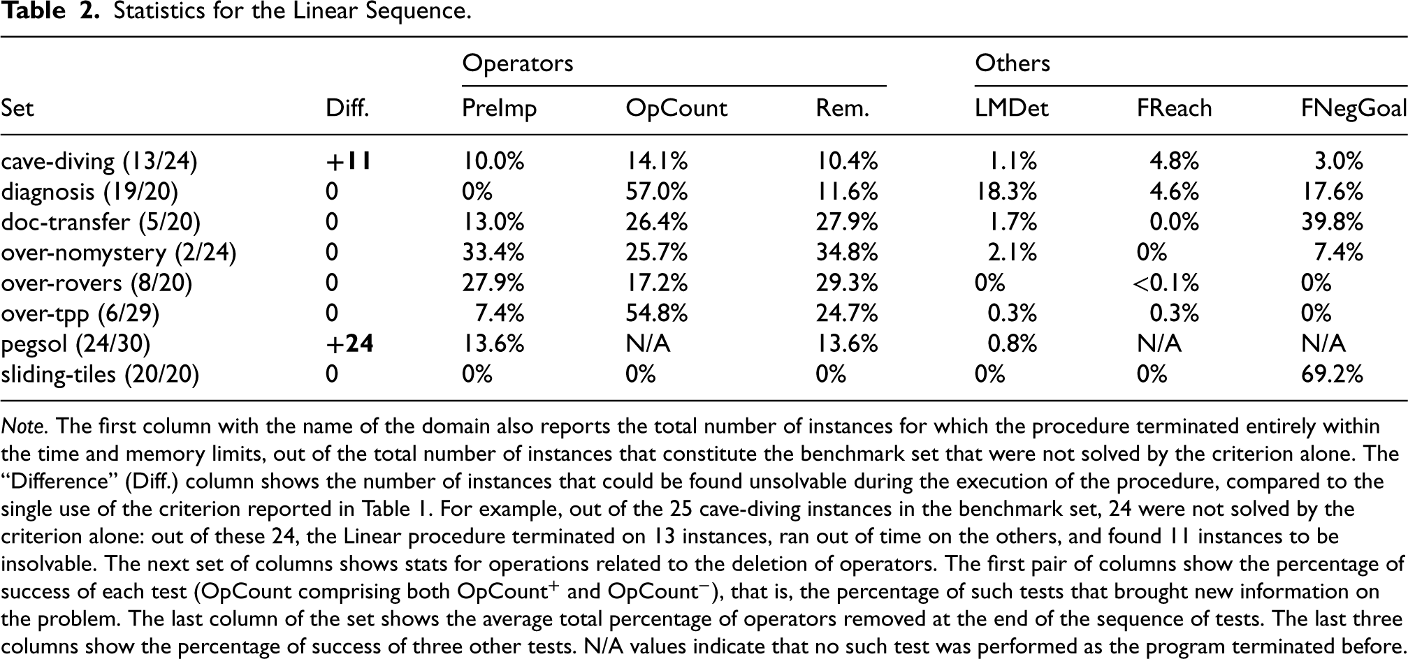
Statistics for the Linear Sequence.
Note. The first column with the name of the domain also reports the total number of instances for which the procedure terminated entirely within the time and memory limits, out of the total number of instances that constitute the benchmark set that were not solved by the criterion alone. The “Difference” (Diff.) column shows the number of instances that could be found unsolvable during the execution of the procedure, compared to the single use of the criterion reported in Table 1. For example, out of the 25 cave-diving instances in the benchmark set, 24 were not solved by the criterion alone: out of these 24, the Linear procedure terminated on 13 instances, ran out of time on the others, and found 11 instances to be insolvable. The next set of columns shows stats for operations related to the deletion of operators. The first pair of columns show the percentage of success of each test (
In the cases where our procedure could not conclude, it still manages to gather valuable information about the planning instance. For example, on some domains, almost a third of all operators are pruned on average, among instances on which our procedure terminates.
The termination of our procedure is, however, the main issue of this sequence of operations, which is too computationally costly, and often stops early because of the time and memory limits imposed. In some domains, very few instances could be run through the entire sequence of operations: such domains include over-nomystery, where this sequence terminated on only two instances out of the 24 that could be parsed.
Quadratic sequence
Table 3 shows statistics for the quadratic sequence. As the first part of the quadratic sequence consists of the exact same sequence of operations as the linear sequence, there are at least as many instances solved by the quadratic sequence as by the linear sequence. This is why domains cave-diving and pegsol only exhibit instances that are entirely solved: our procedure detects these instances as unsolvable before reaching the
Statistics for the Quadratic Sequence.
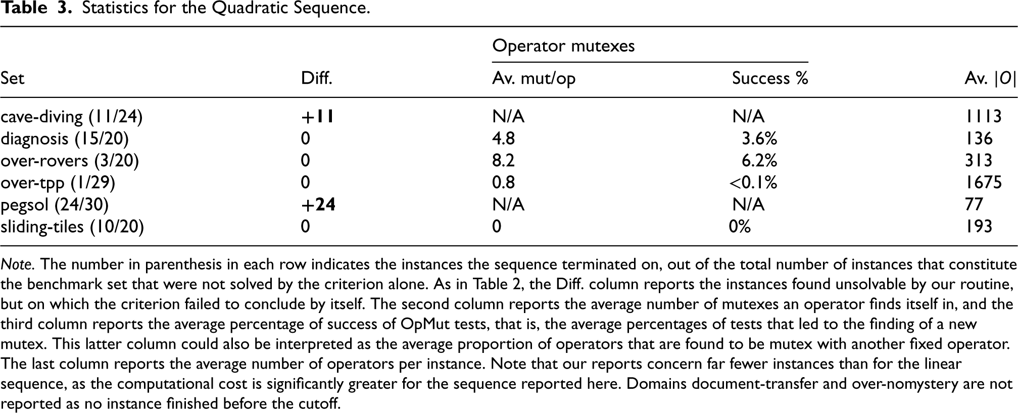
Note. The number in parenthesis in each row indicates the instances the sequence terminated on, out of the total number of instances that constitute the benchmark set that were not solved by the criterion alone. As in Table 2, the Diff. column reports the instances found unsolvable by our routine, but on which the criterion failed to conclude by itself. The second column reports the average number of mutexes an operator finds itself in, and the third column reports the average percentage of success of
In general, the use of a quadratic number of operations quickly becomes problematic: compared to the linear sequence, the quadratic sequence can be run in its entirety on significantly fewer instances. In addition, very few tests are actually successful, as even with the most receptive instances, only a few percent of all tests succeed. However, the main issue with our sequence of operations is that it considers all pairs of operators, and checks if they can be marked as mutexes. The quadratic number of such tests is then responsible for the computational cost of the sequence, but the test in itself remains an integer program that can be solved almost instantly.
Yet, even if we were to find operators mutexes, they would be hard to reinvest in the linear program. Indeed, to be included in the linear program, an operator mutex
Individual Tests
Tables 4 and 5 summarize the statistics for the other sequences, which mostly consist of a series of one or two of the same operations. However, we do not report comprehensive results for all remaining sequences: indeed, in the case of the OperatorDeadLock sequence, no test answered positively, and no dead-end operator could be found.
Performances of the Operator PreImpossible Sequence.
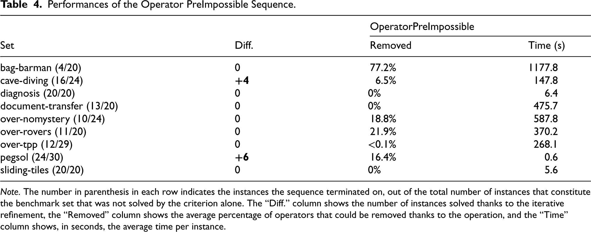
Note. The number in parenthesis in each row indicates the instances the sequence terminated on, out of the total number of instances that constitute the benchmark set that was not solved by the criterion alone. The “Diff.” column shows the number of instances solved thanks to the iterative refinement, the “Removed” column shows the average percentage of operators that could be removed thanks to the operation, and the “Time” column shows, in seconds, the average time per instance.
Performances of the OperatorCount Sequence.
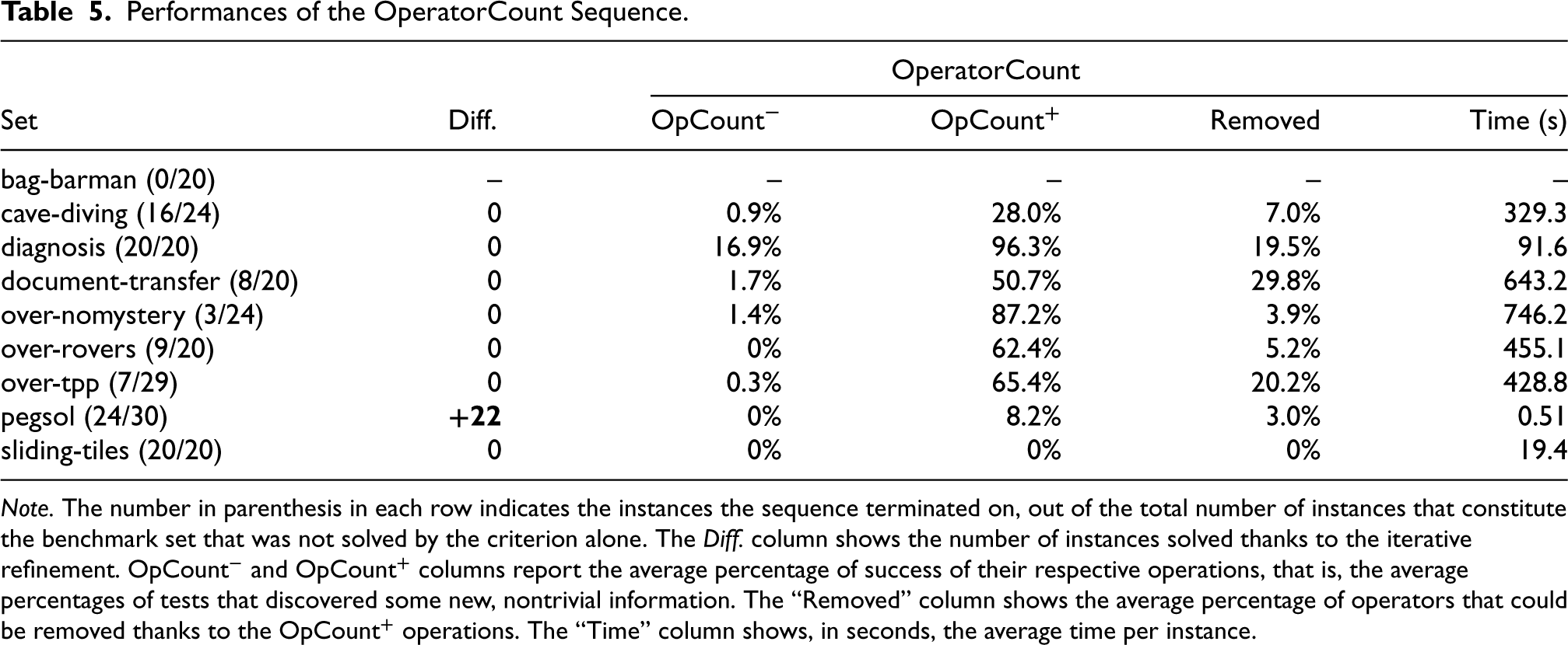
Note. The number in parenthesis in each row indicates the instances the sequence terminated on, out of the total number of instances that constitute the benchmark set that was not solved by the criterion alone. The Diff. column shows the number of instances solved thanks to the iterative refinement.
Nonetheless, the results for the other sequences of operations are encouraging. Be it for the sequence centered on
An interesting property of our
Note that these sequences of tests are not as powerful as the linear sequence, when it comes to detecting unsolvable instances. This seems to indicate that the combination of different kinds of operations is crucial to draw conclusions, and studying their interactions is crucial in designing more powerful sequences.
The surge in interest for unsolvability detection, in the last decade, has been embodied by the first Unsolvability Planning Competition in 2016. The competition saw various adaptations of techniques that have shown themselves efficient for finding plans, in a state space search. Such methods include heuristics specifically tailored for unsolvability detection, such as a Merge & Shrink-based heuristic (Helmert et al., 2014) (which precedes the competition). Such heuristics rely on abstractions that do not preserve distance, but merely solvability.
Another heuristic that was successfully adapted was the operator-counting heuristic (Bonet, 2013; Pommerening et al., 2014; Van Den Briel et al., 2007). The heuristic is based on a relaxation of the orderings of the operators. Previous works showed that it admits an LP formulation, similar to the Linear Program 2 or the Integer Program 1 that we propose. However, while we only optimize the variable associated with the count of a single operator, the objective function that they minimize is the total cost of the plan. The adaptation of the linear program to the case of unsolvability detection was carried out by the Fast Downward-based unsolvability planner Aidos (Seipp et al., 2016). It consists of checking the existence of a solution, in the same way as for Linear Program 2. However, Aidos uses this component in a state space search, in order to detect dead ends.
More generally, be it in unsolvable or in solvable planning tasks, the early detection of states that cannot lead to a goal can help prune out whole branches of the search space. In the case of dead-end detection (Cserna et al., 2018), various works have focused on the elaboration of formulas that can be efficiently evaluated, and whose only models are states that cannot lead to a goal state. The notion of dead-end formula has been generalized with the notion of traps (Lipovetzky et al., 2016): a formula
In the case where our algorithm does not manage to find that the task is unsolvable, it still manages to remove unnecessary elements from the planning model, to make the task easier for the next algorithm. Various other methods prune the model in a preprocessing step: in Alcázar and Torralba (2015), the authors show that invariants in the form of mutexes can be leveraged to remove operators that will never be part of a plan. In Fišer et al. (2019), it is shown how to combine symmetries of the planning task and operator mutexes to find operators that are redundant, in the sense that removing them preserves at least one solution plan.
Our algorithm also learns information that is not explicitly expressible in a STRIPS planning instance. In Steinmetz and Hoffmann (2017b), the authors draw inspiration from a well-known technique in SAT solving, to learn clauses that recognize dead ends, through a conflict-driven approach during search. They also show how to learn traps online Steinmetz and Hoffmann (2017a). Learning is ubiquitous in generalized planning, which is a domain concerned with the synthesis of generalized plans, which are procedures that solve multiple instances. For instance, previous work (Ståhlberg et al., 2021) proposed to learn heuristics in the form of logical formulas, out of a set of small examples instances, so as to recognize unsolvable planning instances.
In Christen et al. (2022), another polynomial criterion is proposed to immediately detect a class of unsolvable instances without resorting to search. The authors synthesize a function that separates the initial state from all goal states, through a linear combination of features valued in a finite field, or at least in a ring. Akin to our criterion, their technique is incomplete, but it is very efficient at detecting parity arguments. In practice, they define a system of linear equations that they solve through a Gaussian elimination process, since the variables have domain
Discussion
Additional Operations
We designed more operations than presented in this paper, but we only report those for which a nontrivial amount of tests answered positively. Operations that never succeeded include operator ordering tests: given
Other such tests include checking if some fluent
Perspectives
Section 5 showed that, when our criterion failed to show an instance unsolvable, it was still possible to extract additional information from the model by leveraging the criterion. Even more so, in some cases, otherwise undetected unsolvable instances could be identified as such by this means. Yet, there is still a lot of room for improvement: a more in-depth study of our operations, as well as their interactions, could help us fine-tune the algorithm, and tailor more effective sequences of operations. Indeed, not all sequences of tests are equal in all aspects, and finding a sequence that avoids unnecessary computations is a way to optimize our algorithm and boost its detection power.
In our tests, we choose to simply run predetermined sequences of operations and tests. This means that, regardless of how tests succeed or fail, the algorithm will linearly go through the same sequence of operations, except if it can show preemptively that an instance is unsolvable. However, the outcome of some tests may help in finding which step to take next. For instance, after finding that an operator is a landmark, it might be interesting to check right away if it can be removed. This can be done through a stack of operations, on which are added the operations that are made relevant by the result of another previous operation.
One of the main weaknesses of our iterative refinement algorithm is its computational cost. Even the most lightweight sequences, such as the OperatorPreImpossible sequence, take significant time to complete. Our program builds each linear program from scratch each time a test is performed. However, very few constraints differ from one linear program to the other; thus, one could modify only these constraints from one test to the next, in order to save significant time. In addition to that, the operations are mostly independent of one another: as a consequence, one could perform multiple operations in parallel with minimum loss.
Finally, as future work, we wish to find a method to reinvest the newly found information about the planning model directly into an off-the-shelf planner, in order to assist it during search. This could either be done by refining the planning model as a preprocessing phase, or by allowing the planner to use our procedure as an oracle during search, to ask very specific questions about some particular aspect of the problem at hand.
Conclusion
In this article, we showed that a simple criterion was sometimes enough to prove that a planning instance is unsolvable. Even though our program is nonoptimized, we have still managed to show that resorting to a search is not always necessary, as reasoning on the model directly can suffice. Even when our procedure fails, it still gathers valuable information about the instance, that provide insight on the planning instance itself.
Other operations and tests can be thought of and included in our framework. The most important point would be to ensure that the information that they bring is related to the other operations (e.g., checking if an operator
Footnotes
Acknowledgments
The authors would like to thank the reviewers of 17èmes Journées d’Intelligence Artificielle Fondamentale for their insightful comments.
Declaration of Conflicting Interests
The authors declared no potential conflicts of interest with respect to the research, authorship, and/or publication of this article.
Funding
The authors disclosed receipt of the following financial support for the research, authorship, and/or publication of this article: This work was supported by the AI Interdisciplinary Institute ANITI, funded by the French program “Investing for the Future—PIA3” under grant agreement no. ANR-19-PI3A-0004..
Appendix A. Sequences of Operations and Tests
Below are shown the exact sequences of operations and tests of each sequence tested on the benchmark sets. Tests that require an argument are run on all possible arguments (e.g.,