Abstract
Understanding reporting behavior in questionnaires is a key issue in enhancing cross-national data comparability and policy decisions. Computers help improve the analysis of careless or insufficient effort (C/IE) responding by logging response times and other response behavior, ensuring data quality. We introduce a response-time based approach, built on an analysis of the relationship between a survey item and a related external variable, to cross-national research. Using PISA 2015 data from 58 countries/economies, we analyze patterns of correlations between the enjoyment of science and science test scores across response time. We focus on C/IE responding towards the beginning of the response time spectrum. Results indicate rather diligent responding in Eastern Asia and a part of Northern Europe. Yet in other regions (e.g., part of Latin America and the Caribbean, and Eastern Europe), C/IE responding might be distorting the data. We provide other researchers with information regarding when and to what extent C/IE responding can occur across countries. We enhance the understanding of heterogeneity in reporting behavior across countries.
Keywords
Introduction
Careless or Insufficient Effort Responding and Computerized Methods of Data Collection
Questionnaire self-report data can be prone to different types of inaccuracies and biases (see, e.g., Duckworth & Yeager, 2015), for example, respondents can be careless or inattentive when responding to items (Curran, 2016; Meade & Craig, 2012). In the literature, the terms careless responding (Meade & Craig, 2012), insufficient effort responding (Huang et al., 2012), and careless or insufficient effort (C/IE) responding (Curran, 2016) to questionnaire items have been used, the issue being widely recognized as a threat to the validity of data. 1 Especially in low-to medium-stakes settings, some participants might not put in the effort to respond accurately or thoughtfully to all questions (Curran, 2016). Such biases might then lead to inaccurate comparisons across different groups of respondents (e.g., across cultures and socioeconomic groups) and hinder the effectiveness of policy decision-making.
The advent of new technologies has notably affected data collection in social science research (Daikeler et al., 2024). Importantly, computerized methods of data collection allow the collection of paradata (i.e., data about the process of answering a questionnaire), which can be used to measure and analyze the quality of responses (Couper, 2005; Matjašič et al., 2018). One type of such paradata is information about questionnaire item response times (Matjašič et al., 2018). Analysis of questionnaire (item) response times have been identified as a promising approach to identify C/IE responding (Curran, 2016; Huang et al., 2012; Meade & Craig, 2012).
Analysis of response times has great utility in the social sciences. International large-scale assessment studies, such as the Programme for International Student Assessment (PISA), which we use in our study, test students’ performance in different subjects (e.g., science, math, and reading) and collect a variety of information concerning noncognitive student factors through context questionnaires (Bertling et al., 2016). The increased interest in noncognitive factors to measure trends, compare subgroups, and evaluate policies places a high demand on the accuracy of their measurement (Bertling et al., 2016). In 2015, PISA collected computer-based data (including both test and questionnaire response time data) across the majority of participating countries/economies (OECD, 2017). Thus, an analysis of these readily available data sets with the aim of identifying C/IE responding might help improve the validity of the PISA findings.
Response Time Analysis and the Identification of C/IE Responders in Questionnaires
Since the use of computers for data collection has grown, the test and questionnaire item response times can be collected more easily. Indeed, numerous studies focusing on the analysis of response times in achievement tests have been published, often focusing on so-called rapid guessing (e.g., Guo et al., 2016; Wise, 2017). Rapid guessing occurs when disengaged test-takers spend too short a time reading and considering the content of an item but still respond to that item (Sahin & Colvin, 2020).
Recently, some studies analyzing questionnaire item response times have focused on attempting to recognize respondents who do not give enough effort to their answer and provide C/IE responses. Zhang and Conrad (2014) call this kind of behavior (i.e., responding too fast to give much thought to answers) “speeding.” However, there is the challenge of how to set the time threshold to identify speeding respondents. Furthermore, there are two additional complications. First, researchers analyzing rapid guessing in a test can examine the appropriateness of a given threshold by analyzing whether the accuracy of test item responses identified as rapid guesses correspond to the rates that could be expected by chance, with the accuracy rates exceeding chance suggesting the inclusion of effortful responses (e.g., Wise & Ma, 2012). However, this objective baseline is absent when analyzing response times to questionnaire items. Second, the response times to a questionnaire are often recorded per web page, which can include many items. As a result, researchers often lack the information about the response time per individual questionnaire item. Both these issues complicate the identification of speeding respondents (i.e., C/IE responders) in questionnaires (Soland et al., 2019).
In the literature, we identified the following approaches to the identification of speeding on questionnaire items. The first approach is the 2s per item approach used by Huang et al. (2012). This threshold was based on their understanding of the survey instructions and items, which the authors believed were unlikely to be responded to faster than the rate of two seconds per item. Similarly, the 2s threshold was adopted by Bulut (2021).
Next approach uses an external, empirically derived threshold. The time threshold for the identification of speeding is supported empirically using other data sets, not the response time data itself. An example of this approach is setting the threshold based on the average reading time of respondents (i.e., the reading time approach). Zhang and Conrad (2014) set the speeding threshold to 300 milliseconds per word multiplied by the number of words in the item, referencing information about the typical reading speed of college students for comprehension.
Another approach uses an internal, empirically derived threshold based on absolute response time value. This approach employs the response time data itself to derive a fixed speeding threshold, all respondents below this absolute response time value being identified as speeders. For example, Greszki et al. (2015) determined a median response time for each survey page and set the threshold for speeding as the time either 30%, 40%, or 50% faster than this median (i.e., the median approach).
Computer-Based Collection of Response Time Data in ILSA Studies
In 2015, PISA collected computer-based data across the majority of participating countries/economies (OECD, 2017). Concerning questionnaire response times, Bulut (2021) focused on engaged and disengaged students in both PISA 2015 tests and questionnaires. Disengaged behavior when responding to a test’s items was distinguished by the normative threshold method (Wise & Ma, 2012) and to the questionnaire’s items by a 2-second threshold according to Huang et al. (2012). If a student showed disengaged behavior in more than 90% of items in the test they were qualified as a disengaged student in the test (the same for the questionnaire). Bulut (2021) found, for example, that disengaged students in the test have the tendency to continue to show disengaged behavior also in the questionnaire.
This Study
We introduce a response-time based approach, built on the analysis of the relationship between a survey item and a related external variable, to cross-national research. We build on Soland et al. (2019) who examined the correlation between respondents’ self-efficacy scores and test scores, in different response time bins, within a single country, as well as the methods that combine response time and accuracy, which is used in rapid guessing literature (Wise, 2017). These methods posit that once respondents’ response time for an item reaches a certain threshold, the accuracy of responses will significantly increase, which is classified as the transition between rapid guessing and solution behavior (Wise, 2017). We examine how the, both theoretically and empirically well-established, relationship between two variables (such as between the enjoyment of science and science achievement; OECD, 2016) changes across response time in different countries. A notably lower correlation between the two variables in the early response times, compared to the later ones, could indicate the presence of careless or insufficient effort responding in the early response times. To the best of our knowledge, this approach to identifying C/IE responding has not been used before in cross-national comparisons.
For each country, we examine the patterns of correlations between the enjoyment of science and science test scores, for students with different response times to the enjoyment of science items. We also focus on the total response time where the correlation between the enjoyment of science and science achievement was not significantly different from zero to identify the span of response times in which the data might be hindered by C/IE responding in a given country. We focus on the beginning of the response time spectrum (up to 22s).
Our analysis could provide other researchers with the information regarding when and to what extent C/IE responding due to fast responding can occur in different countries, allowing them to better target scanning for C/IE responding in their studies. Subsequently, we aim to examine these correlations across groups of countries in different world regions to identify whether there are any consistent patterns. This could enhance our understanding of the link between reporting behavior and cultural/regional differences.
Our research questions are: 1. What is the relationship between students’ self-reported enjoyment of science and science achievement across the response times to the self-reports, in different countries? 2. What are the correlation patterns for the enjoyment of science and science achievement across the response times to the self-reports, in different world regions?
Our approach can be used not only for the enjoyment of science and science achievement, but also has a wide applicability across a range of variables in social science research where respondents’ self-reported attitudes, beliefs, etc., can be related to an external criterion (e.g., achievement test scores).
Methods
Data
We use PISA 2015 data. PISA is conducted by the Organisation for Economic Co-operation and Development (OECD) and tests 15-year-old students’ reading, mathematics, and science literacy (OECD, 2017). The 2015 cycle focused on science literacy and altogether 58 countries/economies participated in a computer-based assessment, collecting data from 447,440 students. For the list of countries/economies 2 with their three letter codes and number of respondents for each country in our analysis, see Table A1 in Appendix. The countries are also divided into specific world regions—we adhere to the list of geographic regions by the Statistics Division of the United Nations (United Nations, 2024).
We analyze students’ responses to the Enjoyment of science question (ST094) from Student questionnaire data file (OECD, n.d.-b). It includes five items with a 4-point Likert scale (1- Strongly disagree, 2- Disagree, 3- Agree, and 4- Strongly agree): 1. I generally have fun when I am learning < broad science > topics. 2. I like reading about <broad science>. 3. I am happy working on < broad science > topics. 4. I enjoy acquiring new knowledge in <broad science>. 5. I am interested in learning about <broad science>.
The wording in angle brackets was chosen by individual countries to fit their national context. Respondents who answered all five items were included. We use the mean of the responses to the five items for the further analysis, calling the variable SEnjoyment.
We also analyze response time for the Enjoyment of science question logged in the Cognitive items total time/visits data file (OECD, n.d.-b). In general, the times logged in this data set are times spent on individual screens in milliseconds. The Enjoyment of science question was displayed to students on one screen.
Finally, as an external variable to identify C/IE responding, we use information about the students’ science achievement. The science achievement test was related to the physical systems content area, the living systems content area, and the earth and space systems content area (OECD, 2016). We employ all of the plausible values for achievement (for details about the calculations, see Monseur & Adams, 2009). Furthermore, we also use the information about overall achievement scores in science, mathematics, and reading (OECD, 2016).
The ethical committee at the authors’ institution provided ethical approval for this research.
Analysis
We aimed at analyzing 3 the countries based on the different patterns of correlations between the enjoyment of science and science test scores, for students with different response times to the enjoyment of science items. We have employed a moving window approach (Henry et al., 2021) where we shift the two-second response time interval by 100 milliseconds (i.e. 0–2s, 0.1–2.1s, 0.2–2.2s, up to 20–22s), aiming to cover the response time continuum. We represent these intervals by the center of the interval (i.e., 1s, 1.1s, 1.2s, up to 21s). For each interval, we calculated a correlation between the students’ SEnjoyment and science achievement (using all 10 plausible values, see data description). The correlation was calculated for the two-second intervals which had at least 40 valid observations (i.e., students that answered all five Enjoyment of science items) in order to ensure sufficient correlation stability (Gnambs, 2023). This approach allowed us to closely observe the correlation development over time. Finally, for each two-second interval, we tested whether the correlation is significantly different from zero. If the correlation in this interval was not significantly different from zero, we label the center of this interval as a Point of Nonsignificant Correlation (NC point). For example, if the correlation is not significantly different from zero in an interval with the center of 4s, it has an NC point of 4s. We then define the NC period as the number of NC points times 0.1s (shift of the moving window), which represents a period during which science achievement and SEnjoyment are not significantly correlated. As an example, a country with 34 NC points has an NC period of 3.4s. Additionally, as correlation non-significance is dependent on the size of the 95% confidence interval, it is necessary to take into consideration the correlation strength and the number of observations, which are the parameters featured in the confidence interval calculation. As such, we discuss both of these parameters in our analysis, alerting readers to them as a possible explanation for a found non-significant correlation.
We studied the first 22 seconds of response times for each country. Previous literature has suggested a 2-second speeding threshold per item (Huang et al., 2012). As our question includes five items, the speeding threshold in our study is 10 seconds. We doubled the theoretical speeding threshold for the five items (20s) in order to capture the correlations for both fast-responding respondents as well as for those with longer response times and added two extra seconds for reading the instruction to the items. We cover all the students who answered all of the five items up to the 22 second response time (N = 219,628). This is 55.62% of all students who answered all of the five items. This proportion differs across countries, with, for example, Korea having 92.91% and the Dominican Republic having 18.84% of students in the 22s response-time spectrum. For country details, see Table A1 in Appendix. Note that only a few students (on average, 6.47 per country) are excluded before the correlations are calculated due to a low number of observations (see Table A2 in Appendix), the maximum being 38 students for Peru. For all countries, the number of observations is lower in the earlier intervals, yet is 500+ in the final interval (center at 21s) for the majority (37 out of 58) of the countries (min. N in the final interval being 116 in Massachusetts [USA]).
For each country we identify the following two criteria: (1) the length of the NC period (i.e., the total time where the correlation between SEnjoyment and science achievement was not significantly different from zero) and (2) the highest correlation between SEnjoyment and science achievement across the response time intervals. The first criterion was set as an indicator of the span of the response time in which the data might be hindered by C/IE responding in a given country. The second criterion was set as an indicator of whether there exists a notable relationship between the enjoyment of science and science achievement in a given country at all. To get a more complex picture of the correlations between science enjoyment and achievement, we also discuss a number of other criteria: at what time the initial interval (i.e., the first interval in which the country had 40 or more respondents and the correlation was computed) occurs, at what time the NC period occurs, at what time the correlation reaches its highest value, in what range of values does each non-significant and significant correlation mostly occur, the correlation strength deciles for individual countries (see Table A2 in Appendix for detailed statistics), and what is the number of observations in the intervals, which is discussed especially in relation to the relatively high, yet non-significant correlations.
Finally, we look at the level of science achievement and SEnjoyment during the NC period compared to the period in which the correlation is significantly different from zero. This illustrates the differences between students who reply during the NC period (i.e., potentially responding carelessly) and those who reply during the period in which the correlation is significant. We also examine the correlation of the length of the NC period, and the size of the peak correlation with the overall science, math, and reading achievement scores of the country (OECD, 2016).
As a robustness check, we have applied the same approach for a moving three-second response time window. We have found that both the length of the NC period, as well as the maximum correlation achieved in the countries, were strongly correlated with the two-second approach (0.949 and 0.967, respectively) and as such, we focus on the two-second variant.
Results
Country/Regional Analysis
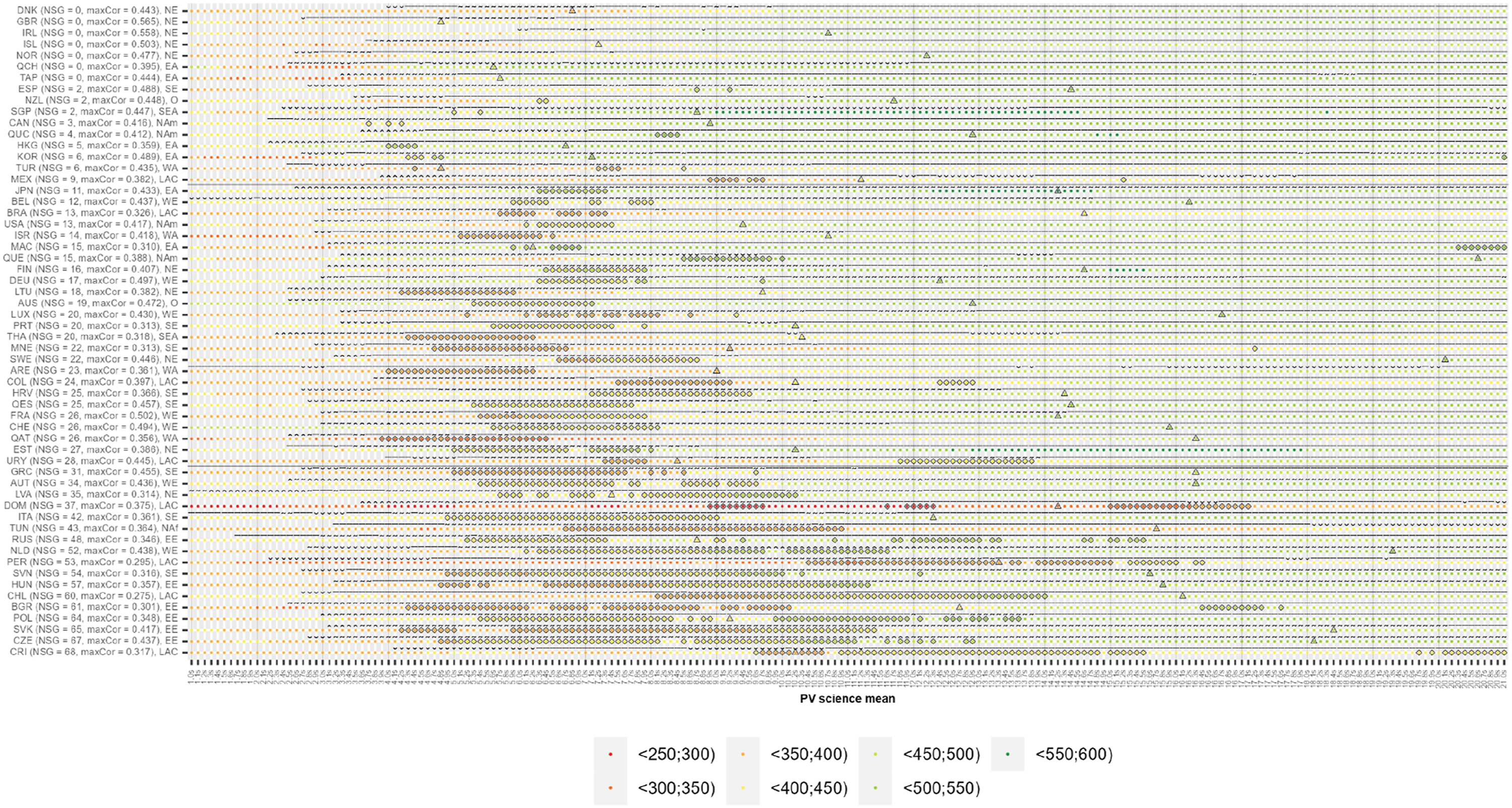
For each country, to get a complex overview, we depict the strength of the correlation, the highest correlation achieved, the number of observations, and the NC period across time (see Figure 1). The correlation strength, the highest correlation achieved, the number of observations, and the NC period across time intervals in each country. Note. Two-second intervals are represented by their center. Triangles represent the maximum correlation. Diamonds represent NC points. ˙ represents N ranging 1–39, ¨ 40–69, ‾ 70–99, ˜ 100–499, ˘ 500+. Correlation strength is represented by colored dots ranging from dark red (negative correlation) to dark green (correlation above or equal to .5). NSG represents the NC period, maxCor represents the highest correlation. NE/EE/WE/SE represent Northern/Eastern/Western/Southern Europe, EA/WA/SEA represent Eastern/Western/South-eastern Asia, NAm represents Northern America, LAC represents Latin America and the Caribbean, NAf represents Northern Africa, and O represents Oceania. For the details on the NC period, max correlation, the initial intervals, observation before the initial interval and the percentage of correlation within individual correlation strength groups, see Table A2 in Appendix.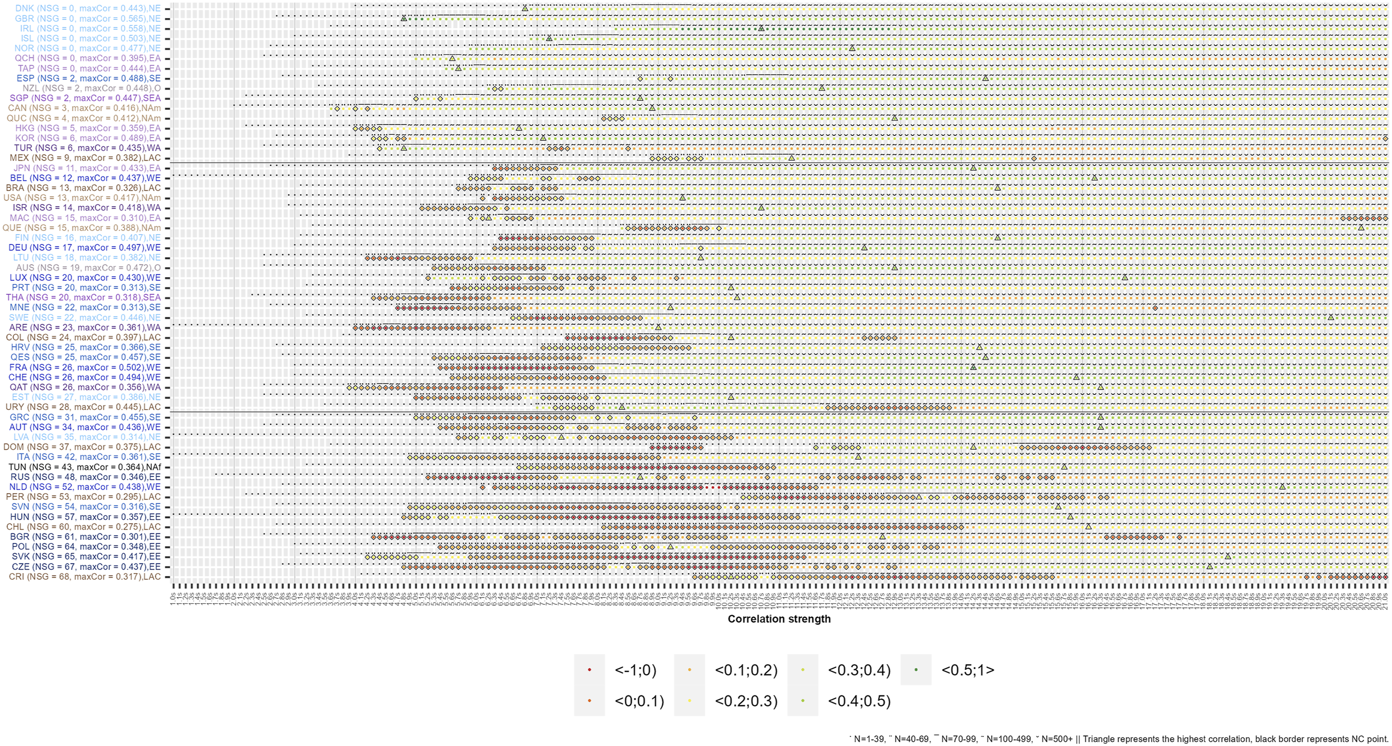
We also provide a scatterplot depiction of countries based on two criteria, the length of the NC period and the size of the highest correlation achieved across countries and world regions (Figure 2). Also, the world maps depicting how different countries score on the two criteria are in the Appendix (Figures A1 and A2). Countries represented based on the length of the NC period and the size of the highest correlation achieved.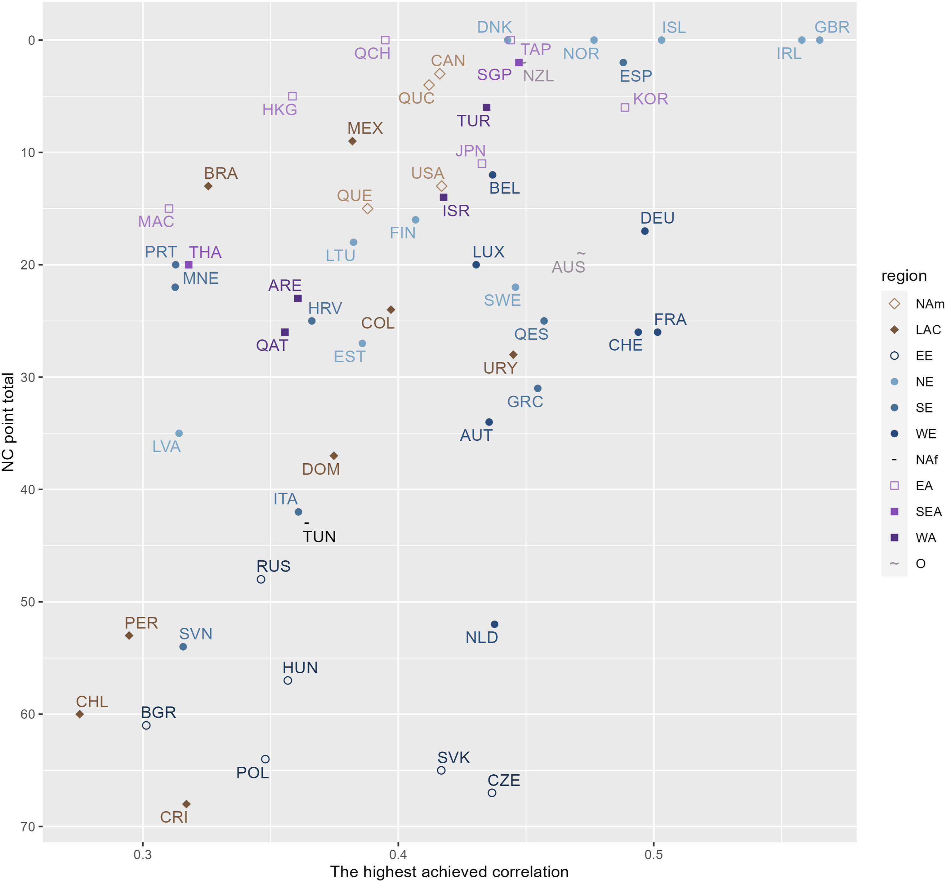
Here, we provide the results for countries and world regions in our dataset.
Eastern Asia
B-S-J-G (China) and Chinese Taipei have no NC period. The initial interval occurs at 5.0 and 5.5s, respectively, the correlations peaking (.395 and .444, respectively) before 6s. The correlations are mostly between .2 and .3 (69.6%) in B-S-J-G (China) and between .3 and .4 (56.4%) in Chinese Taipei. The correlation gets weaker (mostly .1 to .2) from ca. 18 and 19.5s, respectively.
Hong Kong and Korea have 0.5 and 0.6s NC periods, respectively. The initial intervals occur at 4.0 and 4.3s, respectively. The 0.5s NC period runs until 4.4 and 4.8s (scattered in Korea), respectively, the non-significant correlations being between .158 and .272 (the number of observations in intervals N is between ca. 40–120). Concerning significant intervals, the correlations are mainly between .2 and .3 (80.7%) in Hong Kong and between .3 and .4 (40.7%) and .4 and .5 (27.8%) in Korea, peaking (.359 and .489, respectively) around 7s.
Japan and Macau have 1.1 and 1.5s NC periods, respectively. In Japan, the NC period occurs between the initial interval (6.3s) and 7.3s, most (72.7%) correlations being between .15 and .20. Significant correlations are mainly between .3 and .4 (86.9%), peaking (.433) at 14.2s. In Macau, two parts of the NC period occur: (1) scattered between the initial interval (5.9s) and 6.9s (non-significant correlations between .176 to .217, N = 41–103) and (2) between 20.3 and 21.0s with correlations about .1. Significant correlations are mostly between .2 and .3 (83.9%). The peak (.310) at 6.2s is surrounded by the NC period.
South-Eastern Asia
Singapore has an NC period of 0.2s, which occurs at the initial interval (5s) and at 5.4s, with correlations .300 (N = 40) and .260 (N = 55), respectively. Significant correlations are mostly between .3 and .4 (64.2%), peaking (.447) at 8.7s.
In Thailand, the NC period is 2.0s and occurs between the initial interval (4.3s) and 6.2s with correlations between .05 and .15. Significant correlations are mostly between .1 to .2 (49.3%) and .2 to .3 (45.3%), peaking (.318) at 10.3s.
Western Asia
Turkey has an NC period of 0.6s which is scattered from the initial interval (4.4s, .287, N = 49) through 7.2–7.5s (correlations about .1) to 8.5s (.105). Significant correlations are mostly between .1 to .2 (67.7%) and .2 to .3 (24.2%, mostly around 6s and between ca. 16.5–18.5s), peaking (.435) at 4.8s.
Israel has an NC period of 1.4s scattered between the initial interval (5.1s) and 6.5s, with correlations mostly between .1 and .2 (85.7%). Significant correlations are mostly between .2 to .3 (62.3%) and .3 to .4 (27.4%), peaking (.418) at 10.7s.
The United Arab Emirates (UAE) and Qatar have an NC period of 2.3s and 2.6s, respectively. The NC period occurs between the initial interval (4.0s and 3.9s, respectively) and 6.2s and 6.4s, respectively. In the UAE, most of the non-significant intervals range between −.05 to .10 (87.0%) while in Qatar, most (88.5%) are between .05 and .15. In the UAE, significant correlations mostly occur between .2 and .3 (72.3%), peaking at 9.0s (.361). In Qatar, significant correlations are mostly between .2 to .3 (51.4%) and .3 to .4 (36.3%), peaking at 16.3s (.356).
Northern America
Canada and Massachusetts (USA) have an NC period of 0.3 and 0.4s, respectively. In Canada, the initial interval occurs at 3.6s. The NC period occurs scattered between 3.7s and 4.2s, with non-significant correlations .294 (N = 46), .220 (N = 67), and .192 (N = 78). Significant correlations are mostly between .3 to .4 (68.0%) and .2 to .3 (25.6%), peaking (.416) at 8.9s. In Massachusetts (USA), the NC period occurs between the initial interval (8.1s) and 8.4s, ranging from .183 to .265 (N = 47–52). Significant correlations are mostly between .3 to .4 (54.0%) and .2 to .3 (42.9%), peaking (.412) at 12.9s.
The USA and North Carolina (USA) have an NC period of 1.3 and 1.5s, respectively. In the USA, the NC period occurs between the initial interval (6.1s) and 7.4s with one interval (6.2s) where correlations were not computed (N < 40). The nonsignificant correlations are mostly (84.6%) between .15 and .25 (N = 40–81). Significant correlations are mostly between .2 to .3 (47.8%) and .3 to .4 (47.1%), peaking at 9.4s (.417). In North Carolina (USA), the initial interval occurs at 8.4s. The NC period occurs scattered between 8.5s and 10.0s, correlations mostly ranging from .05 to .15 (73.3%). Significant correlations are mostly between .2 to .3 (49.1%) and .3 to .4 (41.1%), peaking at 20.6s (.388).
Latin America and the Caribbean
Mexico and Brazil have NC periods of 0.9 and 1.3s, respectively. In Mexico, the majority of the scattered NC period occurs between the initial interval (8.9s) and 9.7s with the correlations from .208 to .273 (N = 40–54) with one non-significant interval also reoccuring at 15.2s (.133). Significant correlations are mostly between .2 to .3 (46.0%) and .3 to .4 (31.0%), peaking (.382) at 11.2s. In Brazil, the scattered NC period occurs between the initial interval (5.7s) and 7.3s with most of the correlations between .1 to .2 (92.3%). Significant correlations are mainly between .2 and .3 (86.5%), peaking (.326) at 14.6s.
Colombia and Uruguay have NC periods of 2.4 and 2.8s, respectively. The initial interval occurs at 7.5 and 7s, respectively. In Colombia, two parts of the NC period occur: (1) between 7.5 and 9.2s with the correlations from −.087 to .061 up till 8.7s followed by correlations ranging from .123 to .203 up till 9.2s, (2) between 12.4 and 12.9s with the correlations between .118 to .144. Significant correlations are mostly between .2 to .3 (58.0%) and .1 to .2 (30.4%), peaking (.397) at 10.2s. In Uruguay, the NC period also occurs in two parts: (1) between 7.3 and 7.9s with correlations from .203 to .275 (N = 43–50), and (2) between 11.8 and 13.8s with correlations from .030 to .166 (N = 107–181). Significant correlations are mostly between .2 to .3 (47.8%) and .3 to .4 (28.3%), peaking (.445) at 8.4s.
The Dominican Republic has an NC period of 3.7s. The initial interval occurs at 8.9s and there is a gap (9.8 to 11.5s) with no correlations computed (N < 40). The NC period is divided into 3 parts: (1) between 8.9 and 9.7s with the correlations ranging from −.083 to .062, (2) scattered between 11.6 and 12.3s with correlations between .221 to .315 (N = 40–55), and (3) between 15.0 and 17.1s with varied, mostly low correlations between .1 and .2. Significant correlations are between .2 to .3 (58.2%) and .3 to .4 (41.8%), peaking (.375) at 14.2s. Note that 655 students responded within 22s to all five items (which is 19% of all students with answers to all five items in the PISA sample for the Dominican Republic). The total number of analyzed observations is, compared to other countries, the lowest and is reflected in the correlation pattern (e.g., high yet non-significant correlations in the second part of the NC period).
Peru, Chile, and Costa Rica have NC periods of 5.3, 6.0, and 6.8s, respectively. In Peru, from the initial interval (10.4s) up till 16.4s, the scattered NC period occurs with the non-significant correlations mainly between .1 to .2 (58.5%) and 0 to .1 (20.8%). Significant correlations are between .2 to .3 (51.9%) and .1 to .2 (48.1%). The peak (.295) at 13.3s is surrounded by the NC period. In Chile, the NC period occurs between the initial interval (8.1s) and 14s with most correlations being between .05 to .15 (70.0%) or lower/negative (25.0%). Significant correlations are mostly between .2 to .3 (97.1%), peaking (.275) at 16.1s. In Costa Rica, the NC period consists of two parts: (1) scattered between the initial interval (9.6s) and 15.5s, the non-significant correlations being mostly (77.8%) between .15 to .25 (N = 40–90) till 11.6s and mostly (71.1%) between .05 to .15 (N = 92–253) till 15.5s and (2) scattered between 19.7 and 21s, the non-significant correlations being mostly between 0 to .1 (75%). Significant correlations are mostly between .1 and .2 (76.6%), peaking (.317) at 10.2s.
Northern Europe
Denmark, Great Britain, Iceland, Ireland, and Norway have no NC period. Their initial intervals start at 4.8s (Great Britain), 5.9s (Norway), 6.8s (Denmark), 6.9s (Iceland), and 8.3s (Ireland). In Denmark, Great Britain, and Iceland, most correlations are between .3 to .4 (68.5%, 66.9%, and 50.7%, respectively; in Iceland, this is followed by the .4 to .5 range with 32.4%). In Norway and Ireland, the correlations are mostly between .4 to .5 (45.4% and 41.4%, respectively) and .3 to .4 (40.1% and 33.6%, respectively). The peak correlations range from .443 in Denmark to .565 in Great Britain and either occur in the initial interval (Denmark, Great Britain), shortly thereafter (Iceland), or later after the initial interval (Ireland at 10.7s, Norway at 12.2s).
Finland, Lithuania, and Sweden have the NC period of 1.6s, 1.8s, and 2.2s, respectively. The NC period occurs at the beginning, between their initial intervals (6.4s, 4.2s, and 6.6s, respectively) and 7.9s, 5.9s, and 8.7s, respectively. In Finland, the NC period starts with four negative correlations yet the last eight intervals range between .164 and .213 (N = 67–93). In Lithuania and Sweden, the non-significant correlations are mostly between .1 to .2 (55.6% and 45.5%, respectively) and 0 to .1 (38.9% and 36.4%, respectively). Significant correlations are mostly between .2 to .3 in Lithuania (64.2%) and between .3 to .4 in Finland (67.2%) and Sweden (56.1%, followed by the .4 to .5 range with 29.3%). Peak correlations occur at 9.7s for Lithuania (.382), 14.6s for Finland (.407), and 20.1s for Sweden (.446).
Estonia and Latvia have the NC periods of 2.7s and 3.5s, respectively. Estonia has the NC period scattered between the initial interval (5.0s) and 8.0s, the non-significant correlations being mostly (66.7%) between .1 and .2. Significant correlations are mostly between .3 and .4 (64.9%), peaking (.386) at 10.2s. Latvia has a scattered NC period between the initial interval (5.7s) and 10.2s, non-significant correlations ranging .041 to .281, N = 41–107). Significant correlations are mostly between .2 and .3 (83.2%). The peak (.314) at 7.4s is surrounded by the NC period.
Eastern Europe
Russia has an NC period of 4.8s occurring in three main parts: (1) between the initial interval (5.2s) and 7.3s with mostly (63.6%) negative correlations, (2) scattered between 11.7s and 13.3s with non-significant correlations being mostly (93.3%) between .05 and .15, and (3) scattered between 14.6s and 15.5s with non-significant correlations around .1. Significant correlations are mostly between .1 to .2 (64.0%) and .2 to .3 (28.8%), including the peak correlation (.346) at 8.7s.
Hungary has an NC period of 5.7s divided into two parts: (1) scattered between the initial interval (4.8s) and 5.5s with non-significant correlations between .158 and .274 (N = 40–59) and (2) from 6.4 to 11.3s with correlations being mostly (70.0%) below .05 and even negative. Significant correlations are mostly between .2 to .3 (75.5%), peaking (.357) at 15.8s.
Bulgaria, Poland, Slovakia, and the Czech Republic have NC periods of similar lengths—6.1, 6.4, 6.5, and 6.7s, respectively. In Bulgaria, the NC period is divided into two parts: (1) scattered from the initial interval (4.3s) to 10.1s with non-significant correlations mainly between .05 and .15 (64.0%) and (2) scattered between 16.4s and 17.6s, mostly ranging between .05 and .10 (90.9%). Significant correlations are mostly between .1 to .2 (70.1%) and .2 to .3 (29.0%), peaking (.301) at 12.7s. In Poland, the scattered NC period is from the initial interval (5.4s) to 13.6s with non-significant correlations mostly between .1 and .2 (76.6%). Significant correlations are mainly between .2 to .3 (60.2%) and .1 to .2 (28.0%), peaking (.348) at 9.2s. In Slovakia, the NC period consists of two parts: (1) between the initial interval (4.2s) and 5s with correlations between .235 and .283 (N = 41–79) and (2) between 5.9 and 11.4s with correlations mostly (67.9%) below .05 and even negative. Significant correlations are mostly between .2 to .3 (53.8%) and .3 to .4 (38.5%), peaking (.417) at 18.4s. In the Czech Republic, the scattered NC period is between the initial interval (4.8s) and 12.9s with the non-significant correlations being mostly between 0 to .1 (52.2%) and .1 to .2 (37.3%). Significant correlations are mostly between .3 and .4 (64.6%), peaking (.437) at 18.1s.
Western Europe
In Belgium, the NC period is 1.2s, occurring in three parts: (1) between the initial interval (5.9s) and 6.4s, correlations up to .300 (N = 41–48), (2) between 7.1s and 7.2s with correlations around .220 (N = 70–71), and (3) between 7.7s and 8.0s, correlations ranging from .171 to .205 (N = 84–87). Significant correlations are mostly between .3 to .4 (48.6%) and .2 to .3 (22.9%), peaking (.437) at 16.2s.
Germany and Luxembourg have NC periods 1.7s and 2.0s, respectively. In Germany, the NC period mainly occurs scattered between the initial interval (6.3s) and 7.9s, with correlations ranging .067 to .260 (N = 42–60), and one non-significant correlation (.201, N = 77) occurring later (9.7s). Significant correlations are mostly between .4 to .5 (63.4%), peaking (.497) at 12.4s. Luxembourg has its initial interval at 5.2s. The majority of the scattered NC period occurs between 6.1 to 8.1s (ranging from .10 to .25, N = 60–126) with other single non-significant correlations occurring at 5.2s (.198), 8.6s (.177), and 9.3s (.163). Significant correlations are mostly from .3 to .4 (54.0%) and .2 to .3 (28.8%), peaking (.430) at 16.7s.
France and Switzerland have an NC period of 2.6s, which occurs between their initial intervals (5.4s and 5.6s, respectively) and 7.9s and 8.1s, respectively. Non-significant correlations mostly range from −.20 to .05 in France (73.1%) and .10 to .15 in Switzerland (69.2%). Significant correlations are mostly between .4 to .5 (55.7% for France and 48.8% for Switzerland) and .3 to .4 (24.4% and 37.2%, respectively), peaking at 14.2s in France (.502) and 15.9s in Switzerland (.494).
Austria has a scattered NC period of 3.4s occurring between the initial interval (5.4s) and 9.6s, with non-significant correlations ranging from .039 and .224 (N = 40–146). Significant correlations are mostly between .3 to .4 (61.8%) and .4 to .5 (24.4%), peaking (.436) at 16.3s.
In the Netherlands, the initial interval occurs at 6.1s. The NC period of 5.2s occurs scattered between 6.1s and 11.6s, correlations fluctuating between −.128 to .213 (N = 40–344). Significant correlations are mostly between .3 to .4 (63.9%) and .4 to .5 (15.5%), peaking (.438) at 19.3s. Note that in three intervals (9.8 to 10.0s), the negative correlations (around −.15) reached significance.
Southern Europe
Spain has the NC period of 0.2s, the two nonsignificant correlations being .286 at 8.7s (the initial interval, N = 41) and .276 at 9.2s (N = 45). Significant correlations are mostly between .4 to .5 (61.5%) and .3 to .4 range (37.7%), peaking (.488) at 14.4s
Portugal and Montenegro have an NC period of 2.0 and 2.2s, respectively. In Portugal, the NC period mainly occurs between the initial interval (5.6s) and 7.4s (additional non-significant interval occurs at 7.9s), the non-significant correlations fluctuating between .050 and .219. Significant correlations are mostly between .2 and .3 (91.1%), peaking (.313) at 10.2s. Montenegro has the NC period mainly between the initial interval (4.7s) and 6.7s, non-significant correlations being typically negative (40.9%, all occurring till 5.5s) and between .10 and .15 (45.5%). Significant correlations are mostly between .2 to .3 (58.5%) and .1 to .2 (38.7%), peaking at 9.2s (.313).
Croatia and Spain (Regions) both have an NC period of 2.5s. In Croatia, the NC period occurs between the initial interval (7.1s) and 9.5s, correlations ranging from .109 to .247 (N = 43–98). Significant correlations are between .2 to .3 (53.9%) and .3 to .4 (46.1%), peaking at 14.3s (.366). In Spain (Regions), the NC period occurs between the initial interval (5.3s) and 7.7s, correlations ranging from .029 to .245 (N = 42–144). Significant correlations are mostly between .3 to .4 (58.6%) and .4 to .5 (33.1%), peaking (.457) at 14.4s.
Greece has an NC period of 3.1s with the main part being between the initial interval (5.0s) and 7.6s, ranging from .039 to .228 (N = 43–86), and four further non-significant correlations ranging from .203 and .225 occurring scattered between 8.0s and 9.6s (N = 79–98). Significant correlations are mostly between .3 to .4 (55.4%) and .4 to .5 (20.8%), peaking (.455) at 16.3s.
Italy has an NC period of 4.2s between the initial interval (4.9s.) and 9.0s, ranging .033 to .246 (N = 43–189). Significant correlations are mostly between .2 to .3 (65.0%) and .3 to .4 (32.5%), peaking (.361) at 12.3s.
Slovenia has an NC period of 5.4s, the majority of which occurs between the initial interval (4.9s) and 10.0s, with correlations ranging from −.012 to .241 (N = 40–159), with two more non-significant intervals at 10.3s (.147) and 12.1s (.106). Significant correlations are mostly between .2 and .3 (75.9%), peaking (.316) at 15.6s.
Oceania
New Zealand has an NC period lasting 0.2s. The initial interval starts at 6.2s. The NC period occurs at 6.3–6.4s with correlations about .270 (N = 42–43). Significant correlations are mostly between .3 to .4 (46.3%) and .4 to .5 (40.8%), peaking (.448) at 11.7s.
In Australia, the NC period is 1.9s and occurs between the initial interval (5.3s) and 7.1s with the correlations mostly between .05 to .15 (73.7%). Significant correlations are mostly between .3 to .4 (55.4%) and .4 to .5 (42.4%), peaking (.472) at 12.9s.
Northern Africa
Tunisia has an NC period of 4.3s between the initial interval (6.7s) and 10.9s. The NC period starts with four correlations above .2 (N = 43–51), yet most values range from negative to .1 (65.1%). Significant correlations are mostly between .2 to .3 (69.3%) and .3 to .4 range (29.7%), peaking (.364) at 15.7s.
Science Achievement and Enjoyment in Relation to Response Time, NC Period, and Maximum Correlation
In all countries, we find that the intervals with the lowest country achievement (specifically the 5% of the intervals with the lowest achievement in science) are typically those which occur relatively early. The only exceptions were Ireland, Massachusetts (USA), and North Carolina (USA), where some of these intervals appeared later. Concerning the enjoyment of science, for the majority of countries, the intervals with the lowest country enjoyment of science (specifically the 5% of the intervals with the lowest enjoyment of science) also typically occur early. However, for some countries this is not the case. For example, for Belgium, Germany, Hungary, Iceland, Israel, New Zealand, Slovenia, Switzerland, Turkey, and Uruguay, the majority of intervals with 5% of the lowest enjoyment of science were found in their middling significant time intervals. For more information on achievement in science and enjoyment of science levels across time intervals for all countries, see Figure A3 in the Appendix.
Further, when we consider the differences between respondents in the NC period and outside of the NC period, we have found that for each country with an NC period, respondents in the NC period had a lower mean science achievement compared to those in intervals with significant correlation (the average difference being around 59.47 points, with the PISA score standard deviation being 100 points for OECD countries; OECD, 2016). In the majority of countries with an NC period, respondents in the NC period also reported a lower enjoyment of science than those in significant correlation intervals (the average difference being around 0.17 on a 1 to 4 scale). However, this trend was reversed, for example, in Germany, where NC period enjoyment was 2.90 compared to 2.77 in significant correlation intervals.
We also explored the country-level correlation between science achievement scores and NC period/maximum correlation. For the NC period, the correlation was −.346 (p < .01), suggesting less bias in higher-achieving countries. The correlation between achievement scores and maximum correlation was .403 (p < .01).
Discussion
C/IE Responding in Countries characterized and World Regions in Our Study
Eastern Asian countries can be characterized by rather diligent responding. Possible minor data distortions due to C/IE responding might occur in early intervals 4 . For example, lower correlations (mostly between .15 and .2) appear in the 1.1s long NC period compared to the significant correlations (mostly between .3 and .4) in Japan or are fluctuating (between .158 and .272) in NC periods in early intervals (0.5s) in Hong Kong and Korea. In Vonkova et al. (2018), the analysis using the overclaiming technique based on respondents’ rating of their familiarity with existing and non-existing items, revealed that respondents in this region report significantly lower familiarity with non-existing items relative to their ratings of existing items compared to other regions. Our findings together with those of Vonkova et al. (2018) both indicate an attentive way of responding in this region. Muszyński et al. (2023) found that fast-responding respondents scored high on non-existing items. Another potential indicator of C/IE responding is noncontingent responding, measuring the tendency of respondents to answer differently to similar items. Buckley (2009), using data from countries/economies participating in PISA 2006, found that countries from Eastern Asia scored among the lowest in his sample. Using a composite index of careless responding (based on e.g., longstringing and Mahalanobis distance), Grau et al. (2019) found in their marital satisfaction study in 34 countries that Japanese adult respondents achieved middling index value.
Concerning other regions in Asia, in South-eastern Asia, C/IE responding does not seem to affect data quality in Singapore (only two non-significant, quite high correlations with low N) yet may affect early response-time intervals in Thailand, where the correlations in the 2.0s long NC period are often quite low (below .1) compared to almost half of the significant correlations between .2 to .3. In Western Asia, C/IE responding seems to be an issue in the early response-time intervals, except Turkey. Correlations in the NC period in the early intervals are often quite low (mostly between .1 to .2 in Israel, .05 to .15. in Qatar, and −.05 to .10 in UAE) compared to the majority of significant correlations between .2 and .3. In Turkey, the highest correlations occur predominantly in the early intervals, and lower correlations, though mainly significant, occur mostly later. Buckley (2009) found, compared to other countries, rather low noncontingent responding in Thailand, middling in Turkey, rather high in Israel, and high in Qatar. For Grau et al. (2019), respondents in Singapore achieved middling and in Turkey rather high scores of careless responding index, compared to other countries.
As for America, in Northern America, Canada and Massachusetts (USA) both have short NC periods (up to 0.4s) with relatively high non-significant correlations between .183 and .294 and low N, indicating at most minor distortions due to C/IE responding. The USA has a longer NC period (1.3s) than Canada and Massachusetts (USA) and the non-significant correlations fluctuate mostly between .15 and .25 with low N. In North Carolina (USA), C/IE responding might slightly distort data in the early intervals. The NC period is longest (1.5s) in this region and the non-significant correlations are lower (mostly between .05 and .15) compared to the significant correlations in the country (mostly above .2). In Latin America and the Caribbean, there appear to be differences in the occurrence of C/IE responding. For example, there seem to be no or minor data distortion in Mexico, with an NC period (0.9s) containing high (above .2) non-significant correlations with low N, and Brazil, with an NC period (1.3s) containing non-significant correlations predominantly lower (mostly between .1 and .2) than significant ones (mostly between .2 and .3). However, many countries have rather long (3.7s to 6.8s) NC periods (the Dominican Republic, Peru, Chile, and Costa Rica) which are sometimes scattered or divided into more parts and, at least in some parts, contain quite low and/or fluctuating non-significant correlations. This indicates that C/IE responding might be distorting the data. Note that in some countries (like Peru and Costa Rica), the peak correlations are rather low (below .3) and a considerable proportion of significant intervals are in the .1 to .2 range. This suggests that the relationship between science enjoyment and achievement might be actually weak or that C/IE responding is widespread across the 22s response-time spectrum.
Buckley (2009) found that, compared to other countries, Canadian and American respondents scored low and rather low, respectively, on noncontingent responding while countries from Latin America and the Caribbean exhibited middling to high values. Further, Grau et al. (2019) found, compared to other countries, low careless responding index values in the United States and high values in Latin American countries such as Brazil, Ecuador, and Guatemala. Thus, in Latin America and the Caribbean, there seem to be more respondents not responding to questionnaire items in a careful and attentive manner, warranting a careful investigation of C/IE responding and its effect on the observed relationship between variables in these countries.
As for the European regions, among the studied Northern European countries, Denmark, Great Britain, Iceland, Ireland, and Norway have no NC period and quite strong significant correlations. This indicates rather diligent responding. Finland, Lithuania, and Sweden have NC periods (1.6s to 2.2s) in early intervals which contain notably lower correlations (fluctuating from negative to .213 in Finland, mostly between .1 to .2 and 0 to .1 in Lithuania and Sweden) compared to the significant intervals (mostly between .2 and .3 in Lithuania and between .3 and .4 in Finland and Sweden). This indicates a possible distortion due to C/IE responding in early intervals. Estonia and Latvia have the longest NC periods in Northern Europe (2.7s and 3.5s, respectively), which are scattered. In Estonia, the non-significant correlations are mostly lower (between .1 to .2) compared to the significant ones (mostly between .3 to .4) and in Latvia, the size of non-significant correlations varies .041 to .281 with the peak correlation (.314), which is surrounded by the NC period, occurring at 7.4s. Concerning the Northern European countries with no NC period, Buckley (2009) found that they are among countries with middling to low values of noncontingent responding.
Overall, concerning Eastern Europe, all the countries have quite long NC periods (4.8s to 6.7s). There are parts of the NC period with considerably lower correlations compared to the significant correlations in the respective countries, which is evident especially in Hungary, Slovakia, and the Czech Republic. This indicates that C/IE responding might be distorting the data. In some countries (Russia, Bulgaria), the majority of the significant correlations are quite low (.1 to .2), suggesting that the relationship between science enjoyment and achievement might actually be weak or that C/IE responding is widespread across the studied response-time spectrum. Buckley (2009) found heterogeneity in Eastern Europe, specifically the Czech Republic, Poland, and Slovakia displayed, compared to other countries, low to rather low values of noncontingent responding, while Bulgaria, Hungary, and Russia displayed middling to rather high values. Thus, it is indeed beneficial to observe multiple measures of C/IE responding, as they might bring different information (e.g., Curran, 2016). It might be interesting to investigate noncontingent responding conditionally on different response-time intervals.
Western European countries typically have possible distortions of data due to C/IE responding in early intervals. Belgium has a scattered NC period (1.2s) with rather high (mostly above .2) non-significant correlations with low N, indicating possible minor distortions due to C/IE responding. Germany, Luxembourg, and Austria have scattered NC periods (1.7s, 2.0s, and 3.4s, respectively) with quite varied strength of non-significant correlations (between .067 and .260 in Germany, .10 and .25 in Luxembourg, .039 and .224 in Austria), which are lower than the majority of the significant correlations in the respective countries (between .4 and .5 in Germany and .3 and .4 in Luxembourg and Austria). This points to a possible distortion due to C/IE responding in early intervals in these countries. In France and Switzerland, the non-significant correlations in the NC period (2.6s for both countries) are notably lower (mostly −.20 to .05 in France and .10 to .15 in Switzerland) than the majority of the significant ones (above .3), indicating a possible distortion due to C/IE responding in early intervals as well. The Netherlands has quite a long scattered NC period (5.2s) with considerable fluctuation of non-significant correlation strength (between −.128 to .213), with significant correlations being mostly above .3 (and peaking above .4). This points to a possible data distortion due to C/IE responding across a range of early intervals.
Southern Europe is quite a heterogeneous region in terms of the possible occurrence of C/IE responding. For example, Spain has a very short NC period composed of two relatively high (ca. .28) non-significant correlations with low N, indicating at most minor distortions due to C/IE responding. Montenegro has a longer NC period (2.2s) than Spain and especially early in the NC period, the correlations are negative, while the majority of the significant correlations are between .2 and .3 (and .1 to .2), which points to a possible distortion due to C/IE responding in early intervals. Slovenia has one of the longest NC periods among countries in our study (5.4s) with quite varied strength of non-significant correlations (−.013 to .241) and with most significant correlations between .2 and .3. A possible distortion due to C/IE responding in Slovenia might occur across early response-time intervals. Buckley (2009) also found differences in Southern Europe. In his study, Portugal had low, Croatia, Spain, Greece, and Montenegro had middling, and Slovenia and Italy had rather high to high noncontingent responding values. Grau et al. (2019) found that, compared to other countries, Portugal displayed rather high careless responding values, while Greece and Spain had middling values.
In Oceania, there seem to be at most minor distortions due to C/IE responding in New Zealand (an NC period of 0.2s, high correlations about .270 with low N). Australia has a longer NC period (1.9s) with lower correlations (mostly between .05 and 1.5) compared to the significant ones (mostly above .3), indicating a possible distortion due to C/IE responding in early intervals.
Northern Africa is represented in our study by Tunisia, which has a rather long NC period (4.3s) with most non-significant correlations up to .1, while the significant correlations are mostly above .2. This points to a possible distortion due to C/IE responding across the range of early intervals.
Across the studied countries, the concentration of some of the highest correlations is typically around the time when the peak correlation occurs. This applies to the majority of the studied countries, though the exact time of the occurrence of the peak correlation varies. For example, Singapore has the peak at 8.7s, Brazil with the peak at 14.6, and the Czech Republic with the peak at 18.1s. The cases where the peak is not part of the cluster of the highest correlations are, for example,when the peak occurs in early intervals, surrounded by NC period (e.g., Latvia, Poland, and Peru with peak at 7.4s, 9.2s, and 13.3s, respectively), but the cluster(s) of high correlation appear later.
There should be caution about using a single speeding threshold in cross-country research. For instance, applying a universal 2-second speeding threshold (taken from a threshold applied to the sample of Huang et al., 2012) could wrongly label early responses (under 10–12s for 5 items + initial instruction) as careless in some countries. For example, in Great Britain and Ireland, strong correlations appear early (between 4.8 and 8.3s), suggesting these early responses may not be hindered by C/IE responding. Conversely, in countries like Chile and the Czech Republic, the possible data distortions (e.g., lower non-significant correlation values compared to the significant ones) last, though sometimes scattered, much longer (up to 13–14s).
Responding to Questionnaires and Respondents’ Characteristics
We found negative correlations between NC period length and country science, math, and reading scores (r = −.33 to −.36). This suggests that non-significant correlations towards the beginning of the response time spectrum (up to 22s) are more common in countries with lower achievement. Apart from other explanations, one possibility is that C/IE responding may be more present in countries with lower achievement which may align with the findings of Grau et al. (2019). They argued that higher education, as reflected in the higher Human Development Index (HDI), might make handling questionnaires easier for the respondents. On a sample of adults from 34 countries, they indeed found a strong negative correlation (r = −.62) between their composite index of careless responding and HDI.
Literature has also suggested that response times can differ based on respondents’ characteristics (e.g., education and experience with the internet and surveys; Yan & Tourangeau, 2008) as well as on cultural and linguistic factors (e.g., Meitinger et al., 2021; Shi et al., 2018). Shi et al. (2018) found differences in questionnaire response times among different regions of China, arguing that it reflects the varied backgrounds and habits of participants from different regions when responding to questions. Meitinger et al. (2021) found differences in response latency (the time for reading and reflection before starting to type an answer) between respondents from different countries, with the British taking the least time to start answering, followed by American and German respondents who still had relatively short response latencies, and then Spanish and Mexican respondents with slightly longer response latencies. Based on our findings, we recommend that researchers consider setting different thresholds for different countries and encourage further exploration of the impact of cultural and linguistic factors on response times.
The correlation between science achievement and enjoyment in different countries might be affected by factors other than cultural differences in C/IE responding. For example, teacher practices in science classrooms might affect the relationship between science enjoyment and achievement (though these might also be shaped culturally). Liou (2021) has examined the relationship between science achievement, attitudes, and teacher instructional practices in Taiwan. Liou (2021) documented a significant positive effect of teacher-directed instructional practices and a significant negative effect of inquiry-based instructional practices on science achievement, with inquiry-based instructional practices having more positive predictive power for students’ attitudes toward science than teacher-directed instructional practices.
Conclusion and Limitations
We introduce an approach to analyzing C/IE responding due to speeding in cross-national comparative surveys. We have identified marked differences in the degree to which data from respondents in different countries can be affected by C/IE responding due to speeding. Future research could investigate whether speeding patterns can be extended to other questionnaire items and subsequently to the whole questionnaire. It could also focus on analyzing the stability of students’ reporting behavior patterns using different PISA waves. Furthermore, it could also examine respondents with unusually high response times (as proposed also by Curran, 2016) and compare their characteristics to respondents exhibiting speeding behavior. Finally, research could focus on the collection of other reporting behavior data (e.g., via eye-tracking).
Limitations
Our sample is specific to PISA wave 2015, which involves 15-year-old students, and includes data from countries where computer-administered questionnaires were used. Also, it remains to be investigated to what extent the identified reporting behavior patterns would be the same for adult respondents across different countries, measured concepts, and years. Also, our analysis does not deal with unavailable observations, though the omission of responses might be by itself a sign of C/IE responding. Further, the response time was recorded, as usual with questionnaires, per web page, each including multiple items.
Our approach includes a criterion of correlation significance, which is dependent on both correlation size and the number of observations and both should be considered when analyzing correlation significance. For some of the countries, we discussed this in more detail as there were instances of relatively high, but still non-significant correlations. Finally, when a low correlation appears in an interval, it is debatable whether this is, among other potential causes, due to C/IE responding or due to a weak relationship between enjoyment and achievement, the latter explanation probably being more plausible when low correlations occur in later response-time intervals.
Footnotes
Acknowledgments
We thank Katerina Mayerova for help with reviewing the literature.
Declaration of Conflicting Interests
The author(s) declared no potential conflicts of interest with respect to the research, authorship, and/or publication of this article.
Funding
The author(s) disclosed receipt of the following financial support for the research, authorship, and/or publication of this article: This work was supported by the Czech Science Foundation under Grant GAČR 21-09064S “Heterogeneity in reporting behavior on surveys among different countries, schools and groups of students”.
Ethical Statement
Notes
Appendix
A List of Countries/economies in our Sample With country Codes, the Number of respondents and the Percentage of the Total Available Sample Present in our analysis. Note. Country/economy codes were adapted from PISA 2015 codebook (OECD, n.d.-a). Information on world regions was taken from the United Nations (2024). Concerning the countries/economies which were not specifically mentioned by the United Nations, we sorted B-S-J-G (China) and Chinese Taipei into Eastern Asia, Spain (Regions) into Southern Europe, and Massachusetts (USA) and North Carolina (USA) into Northern America. In total, we work with 219,628 students from 58 countries/economies who answered all five items with a response time up to 22s. N represents the number of respondents whose response time is within 22s and does not include students with missing values, that is, the number of students we analyze in our study. The column “%” represents the percentage of all students who answered all of the five items in each country who we analyzed in our study (i.e., answered all five items within 22s).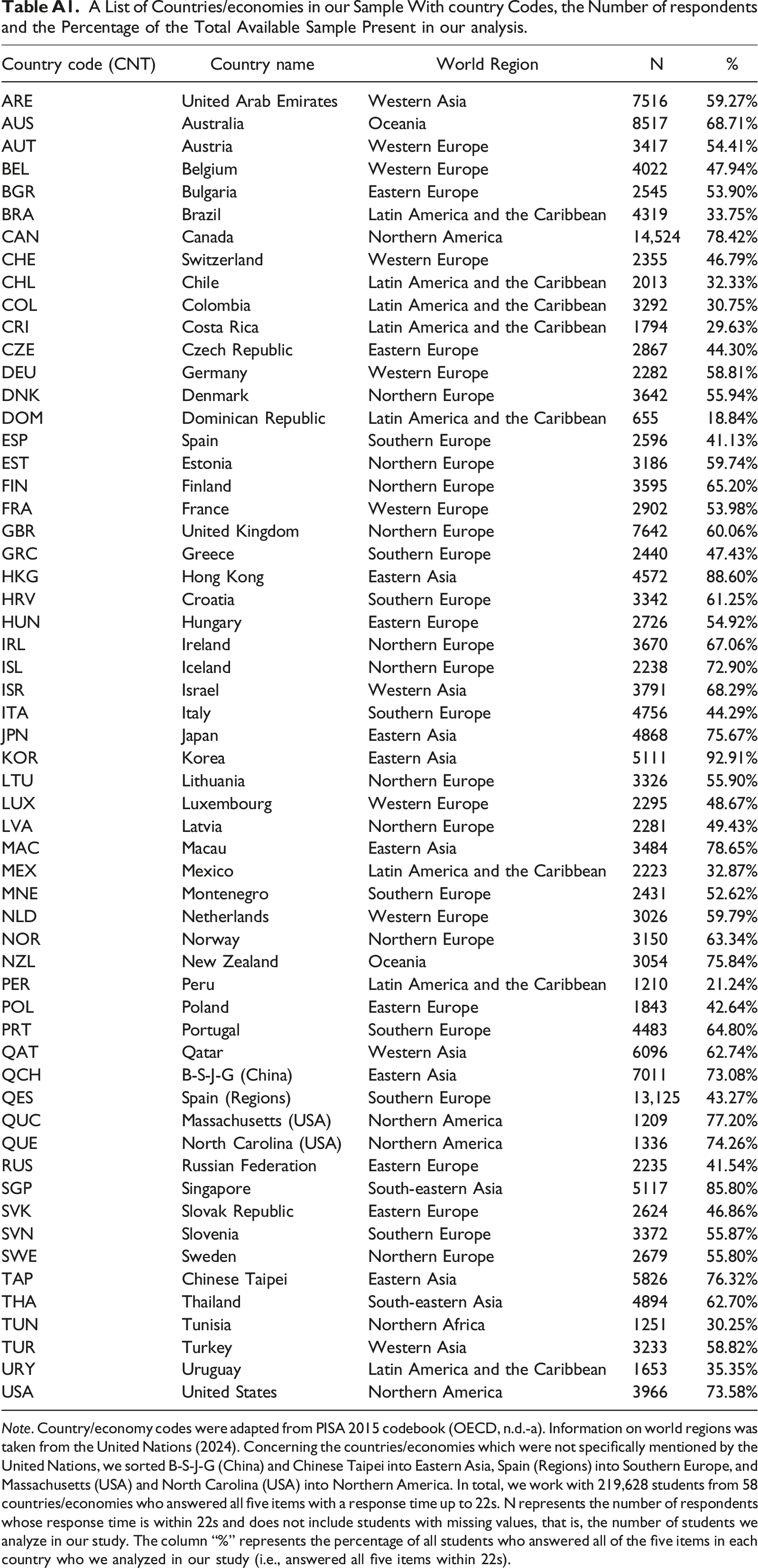
Country code (CNT)
Country name
World Region
N
%
ARE
United Arab Emirates
Western Asia
7516
59.27%
AUS
Australia
Oceania
8517
68.71%
AUT
Austria
Western Europe
3417
54.41%
BEL
Belgium
Western Europe
4022
47.94%
BGR
Bulgaria
Eastern Europe
2545
53.90%
BRA
Brazil
Latin America and the Caribbean
4319
33.75%
CAN
Canada
Northern America
14,524
78.42%
CHE
Switzerland
Western Europe
2355
46.79%
CHL
Chile
Latin America and the Caribbean
2013
32.33%
COL
Colombia
Latin America and the Caribbean
3292
30.75%
CRI
Costa Rica
Latin America and the Caribbean
1794
29.63%
CZE
Czech Republic
Eastern Europe
2867
44.30%
DEU
Germany
Western Europe
2282
58.81%
DNK
Denmark
Northern Europe
3642
55.94%
DOM
Dominican Republic
Latin America and the Caribbean
655
18.84%
ESP
Spain
Southern Europe
2596
41.13%
EST
Estonia
Northern Europe
3186
59.74%
FIN
Finland
Northern Europe
3595
65.20%
FRA
France
Western Europe
2902
53.98%
GBR
United Kingdom
Northern Europe
7642
60.06%
GRC
Greece
Southern Europe
2440
47.43%
HKG
Hong Kong
Eastern Asia
4572
88.60%
HRV
Croatia
Southern Europe
3342
61.25%
HUN
Hungary
Eastern Europe
2726
54.92%
IRL
Ireland
Northern Europe
3670
67.06%
ISL
Iceland
Northern Europe
2238
72.90%
ISR
Israel
Western Asia
3791
68.29%
ITA
Italy
Southern Europe
4756
44.29%
JPN
Japan
Eastern Asia
4868
75.67%
KOR
Korea
Eastern Asia
5111
92.91%
LTU
Lithuania
Northern Europe
3326
55.90%
LUX
Luxembourg
Western Europe
2295
48.67%
LVA
Latvia
Northern Europe
2281
49.43%
MAC
Macau
Eastern Asia
3484
78.65%
MEX
Mexico
Latin America and the Caribbean
2223
32.87%
MNE
Montenegro
Southern Europe
2431
52.62%
NLD
Netherlands
Western Europe
3026
59.79%
NOR
Norway
Northern Europe
3150
63.34%
NZL
New Zealand
Oceania
3054
75.84%
PER
Peru
Latin America and the Caribbean
1210
21.24%
POL
Poland
Eastern Europe
1843
42.64%
PRT
Portugal
Southern Europe
4483
64.80%
QAT
Qatar
Western Asia
6096
62.74%
QCH
B-S-J-G (China)
Eastern Asia
7011
73.08%
QES
Spain (Regions)
Southern Europe
13,125
43.27%
QUC
Massachusetts (USA)
Northern America
1209
77.20%
QUE
North Carolina (USA)
Northern America
1336
74.26%
RUS
Russian Federation
Eastern Europe
2235
41.54%
SGP
Singapore
South-eastern Asia
5117
85.80%
SVK
Slovak Republic
Eastern Europe
2624
46.86%
SVN
Slovenia
Southern Europe
3372
55.87%
SWE
Sweden
Northern Europe
2679
55.80%
TAP
Chinese Taipei
Eastern Asia
5826
76.32%
THA
Thailand
South-eastern Asia
4894
62.70%
TUN
Tunisia
Northern Africa
1251
30.25%
TUR
Turkey
Western Asia
3233
58.82%
URY
Uruguay
Latin America and the Caribbean
1653
35.35%
USA
United States
Northern America
3966
73.58%
An Overview Summary for all Analyzed countries. Note. The country/economy codes were adapted from the PISA 2015 codebook (OECD, n.d.-a). We use a moving window approach where we shift the two-second response time interval by 100 milliseconds (i.e. 0–2s, 0.1–2.1s, 0.2–2.2s, up to 20–22s). The NC period is the total response time out of 22s where the correlation between SEnjoyment and science achievement was not significantly different from zero. Max correlation is the highest correlation between SEnjoyment and science achievement across the response time intervals. Initial interval represents the first two-second interval with computable correlation (i.e. at least 40 observations). Observations before the initial interval represent the number of respondents with an answer to all five achievement motivation items who occurred before the initial interval. For the Dominican Republic, we also include the number of observations in between computed intervals in the Observations before the initial interval. The two-second intervals are represented by their midpoints and are listed in seconds. % of cor is the percentage of all intervals within a country that had at least 40 observations which belong to the listed strength group. NCP% represents the percentage of intervals in the NC period which belong to the listed strength range. SG% represents the percentage of significant intervals which belong to the listed strength range. Angle brackets mean the interval is inclusive of the number next to it.
CNT
NC period
Max Cor
N before the initial interval
Initial interval
Interval with Max Cor
Interval with the first NC point
Interval with the last NC point
% of cor
% of cor ⟨0;0.1)
% of cor
% of cor
% of cor ⟨0.3;0.4)
% of cor ⟨0.4;0.5)
% of cor
ARE
2.3
0.361
1
4.0
9.0
4.0
6.2
2.34%
9.36%
9.94%
62.57%
15.79%
0.00%
0.00%
AUS
1.9
0.472
4
5.3
12.9
5.3
7.1
0.00%
1.90%
8.23%
3.80%
48.73%
37.34%
0.00%
AUT
3.4
0.436
3
5.4
16.3
5.4
9.6
0.00%
3.18%
17.83%
11.46%
48.41%
19.11%
0.00%
BEL
1.2
0.437
10
5.9
16.2
5.9
8.0
0.00%
0.00%
2.63%
26.32%
44.74%
26.32%
0.00%
BGR
6.1
0.301
0
4.3
12.7
4.3
17.6
2.98%
13.69%
64.29%
18.45%
0.60%
0.00%
0.00%
BRA
1.3
0.326
2
5.7
14.6
5.7
7.3
0.00%
0.00%
7.79%
79.87%
12.34%
0.00%
0.00%
CAN
0.3
0.416
0
3.6
8.9
3.7
4.2
0.00%
0.00%
1.71%
26.29%
66.86%
5.14%
0.00%
CHE
2.6
0.494
5
5.6
15.9
5.6
8.1
0.00%
2.58%
14.19%
11.61%
30.97%
40.65%
0.00%
CHL
6.0
0.275
18
8.1
16.1
8.1
14.0
0.77%
28.46%
18.46%
52.31%
0.00%
0.00%
0.00%
COL
2.4
0.397
12
7.5
10.2
7.5
12.9
5.15%
4.41%
32.35%
48.53%
9.56%
0.00%
0.00%
CRI
6.8
0.317
24
9.6
10.2
9.6
21.0
5.22%
21.74%
54.78%
17.39%
0.87%
0.00%
0.00%
CZE
6.7
0.437
1
4.8
18.1
4.8
12.9
4.29%
21.47%
23.31%
6.75%
38.04%
6.13%
0.00%
DEU
1.7
0.497
5
6.3
12.4
6.3
9.7
0.00%
0.68%
6.76%
24.32%
12.16%
56.08%
0.00%
DNK
0.0
0.443
6
6.8
6.8
NA
NA
0.00%
0.00%
0.00%
27.27%
68.53%
4.20%
0.00%
DOM
3.7
0.375
19 + 37
8.9
14.2
8.9
17.1
7.69%
9.62%
12.50%
41.35%
28.85%
0.00%
0.00%
ESP
0.2
0.488
23
8.7
14.4
8.7
9.2
0.00%
0.00%
0.00%
2.42%
37.10%
60.48%
0.00%
EST
2.7
0.386
2
5.0
10.2
5.0
8.0
0.00%
3.11%
11.18%
31.68%
54.04%
0.00%
0.00%
FIN
1.6
0.407
14
6.4
14.6
6.4
7.9
2.72%
2.04%
4.76%
27.89%
59.86%
2.72%
0.00%
FRA
2.6
0.502
4
5.4
14.2
5.4
7.9
8.28%
6.37%
1.91%
15.92%
20.38%
46.50%
0.64%
GBR
0.0
0.565
2
4.8
4.8
NA
NA
0.00%
0.00%
0.00%
3.07%
66.87%
27.61%
2.45%
GRC
3.1
0.455
3
5.0
16.3
5.0
9.6
0.00%
6.83%
6.83%
24.84%
44.72%
16.77%
0.00%
HKG
0.5
0.359
0
4.0
6.7
4.0
4.4
0.00%
0.00%
5.26%
80.12%
14.62%
0.00%
0.00%
HRV
2.5
0.366
20
7.1
14.3
7.1
9.5
0.00%
0.00%
11.43%
50.71%
37.86%
0.00%
0.00%
HUN
5.7
0.357
1
4.8
15.8
4.8
11.3
15.95%
6.75%
8.59%
53.37%
15.34%
0.00%
0.00%
IRL
0.0
0.558
6
8.3
10.7
NA
NA
0.00%
0.00%
0.00%
0.00%
33.59%
41.41%
25.00%
ISL
0.0
0.503
10
6.9
7.2
NA
NA
0.00%
0.00%
0.00%
16.20%
50.70%
32.39%
0.70%
ISR
1.4
0.418
3
5.1
10.7
5.1
6.5
0.00%
0.00%
12.50%
58.13%
25.00%
4.38%
0.00%
ITA
4.2
0.361
10
4.9
12.3
4.9
9.0
0.00%
9.26%
14.81%
51.85%
24.07%
0.00%
0.00%
JPN
1.1
0.433
6
6.3
14.2
6.3
7.3
0.00%
2.03%
5.41%
0.68%
80.41%
11.49%
0.00%
KOR
0.6
0.489
0
4.3
7.1
4.3
21.0
0.00%
0.00%
6.55%
27.38%
39.29%
26.79%
0.00%
LTU
1.8
0.382
0
4.2
9.7
4.2
5.9
0.59%
4.14%
11.24%
57.40%
26.63%
0.00%
0.00%
LUX
2.0
0.430
0
5.2
16.7
5.2
9.3
0.00%
0.00%
11.32%
29.56%
47.17%
11.95%
0.00%
LVA
3.5
0.314
10
5.7
7.4
5.7
10.2
0.00%
6.49%
20.13%
70.13%
3.25%
0.00%
0.00%
MAC
1.5
0.310
4
5.9
6.2
5.9
21.0
0.00%
3.29%
12.50%
78.29%
5.92%
0.00%
0.00%
MEX
0.9
0.382
19
8.9
11.2
8.9
15.2
0.00%
0.00%
22.13%
49.18%
28.69%
0.00%
0.00%
MNE
2.2
0.313
1
4.7
9.2
4.7
17.2
5.49%
1.83%
39.63%
50.61%
2.44%
0.00%
0.00%
NLD
5.2
0.438
6
6.1
19.3
6.1
11.6
19.46%
11.41%
7.38%
10.07%
41.61%
10.07%
0.00%
NOR
0.0
0.477
8
5.9
12.2
NA
NA
0.00%
0.00%
0.00%
14.47%
40.13%
45.39%
0.00%
NZL
0.2
0.448
4
6.2
11.7
6.3
6.4
0.00%
0.00%
0.00%
14.09%
45.64%
40.27%
0.00%
PER
5.3
0.295
38
10.4
13.3
10.4
16.4
4.67%
10.28%
53.27%
31.78%
0.00%
0.00%
0.00%
POL
6.4
0.348
6
5.4
9.2
5.4
13.6
0.00%
7.64%
47.77%
37.58%
7.01%
0.00%
0.00%
PRT
2.0
0.313
4
5.6
10.2
5.6
7.9
0.00%
3.23%
9.03%
82.58%
5.16%
0.00%
0.00%
QAT
2.6
0.356
0
3.9
16.3
3.9
6.4
0.00%
8.72%
15.70%
44.77%
30.81%
0.00%
0.00%
QCH
0.0
0.395
1
5.0
5.6
NA
NA
0.00%
0.00%
23.60%
69.57%
6.83%
0.00%
0.00%
QES
2.5
0.457
4
5.3
14.4
5.3
7.7
0.00%
4.43%
12.03%
6.33%
49.37%
27.85%
0.00%
QUC
0.4
0.412
6
8.1
12.9
8.1
8.4
0.00%
0.00%
0.77%
43.85%
52.31%
3.08%
0.00%
QUE
1.5
0.388
11
8.4
20.6
8.5
10.0
0.00%
5.51%
13.39%
44.88%
36.22%
0.00%
0.00%
RUS
4.8
0.346
4
5.2
8.7
5.2
15.5
8.81%
6.29%
59.75%
20.13%
5.03%
0.00%
0.00%
SGP
0.2
0.447
3
5.0
8.7
5.0
5.4
0.00%
0.00%
0.00%
26.09%
63.35%
10.56%
0.00%
SVK
6.5
0.417
0
4.2
18.4
4.2
11.4
14.20%
14.20%
5.92%
38.46%
23.67%
3.55%
0.00%
SVN
5.4
0.316
1
4.9
15.6
4.9
12.1
1.85%
9.26%
30.86%
54.94%
3.09%
0.00%
0.00%
SWE
2.2
0.446
11
6.6
20.1
6.6
8.7
1.38%
5.52%
6.90%
13.79%
47.59%
24.83%
0.00%
TAP
0.0
0.444
2
5.5
5.7
NA
NA
0.00%
0.00%
8.97%
32.05%
56.41%
2.56%
0.00%
THA
2.0
0.318
1
4.3
10.3
4.3
6.2
0.00%
6.55%
48.81%
39.88%
4.76%
0.00%
0.00%
TUN
4.3
0.364
5
6.7
15.7
6.7
10.9
7.64%
11.81%
8.33%
51.39%
20.83%
0.00%
0.00%
TUR
0.6
0.435
0
4.4
4.8
4.4
8.5
0.00%
0.60%
67.66%
23.95%
5.39%
2.40%
0.00%
URY
2.8
0.445
6
7.0
8.4
7.3
13.8
0.00%
4.26%
22.70%
43.26%
22.70%
7.09%
0.00%
USA
1.3
0.417
6
6.1
9.4
6.1
7.4
0.00%
1.34%
7.38%
46.98%
42.95%
1.34%
0.00%
CNT
cor strength
cor strength decile 1
cor strength decile 2
cor strength decile 3
cor strength decile 4
cor strength decile 5
cor strength decile 6
cor strength decile 7
cor strength decile 8
cor strength decile 9
cor strength decile 10
ARE
−0.029
0.050
0.192
0.222
0.236
0.253
0.269
0.280
0.294
0.306
0.361
AUS
0.088
0.198
0.353
0.365
0.372
0.386
0.397
0.409
0.438
0.454
0.472
AUT
0.039
0.140
0.196
0.267
0.325
0.344
0.361
0.386
0.398
0.410
0.436
BEL
0.155
0.248
0.280
0.306
0.346
0.379
0.389
0.397
0.406
0.416
0.437
BGR
−0.036
0.080
0.113
0.127
0.142
0.152
0.162
0.176
0.191
0.240
0.301
BRA
0.100
0.215
0.249
0.257
0.267
0.277
0.283
0.290
0.295
0.301
0.326
CAN
0.191
0.271
0.288
0.310
0.328
0.338
0.344
0.352
0.361
0.389
0.416
CHE
0.078
0.125
0.267
0.311
0.351
0.380
0.402
0.416
0.451
0.463
0.494
CHL
−0.026
0.031
0.086
0.105
0.141
0.205
0.229
0.240
0.251
0.260
0.275
COL
−0.087
0.120
0.145
0.176
0.194
0.205
0.230
0.247
0.262
0.297
0.397
CRI
−0.029
0.030
0.069
0.109
0.129
0.150
0.163
0.178
0.195
0.218
0.317
CZE
−0.038
0.032
0.076
0.132
0.159
0.216
0.322
0.355
0.367
0.388
0.437
DEU
0.067
0.225
0.275
0.292
0.350
0.414
0.431
0.442
0.450
0.463
0.497
DNK
0.211
0.264
0.287
0.304
0.331
0.340
0.354
0.363
0.372
0.388
0.443
DOM
−0.083
0.024
0.107
0.207
0.237
0.257
0.277
0.290
0.320
0.339
0.375
ESP
0.276
0.330
0.358
0.383
0.401
0.420
0.426
0.435
0.446
0.459
0.488
EST
0.007
0.168
0.218
0.235
0.271
0.309
0.322
0.331
0.344
0.361
0.386
FIN
−0.121
0.203
0.243
0.281
0.309
0.336
0.353
0.367
0.377
0.391
0.407
FRA
−0.203
0.027
0.255
0.298
0.339
0.384
0.420
0.442
0.465
0.474
0.502
GBR
0.261
0.342
0.361
0.369
0.374
0.379
0.388
0.400
0.409
0.418
0.565
GRC
0.039
0.144
0.225
0.251
0.311
0.338
0.356
0.371
0.391
0.425
0.455
HKG
0.180
0.219
0.239
0.247
0.259
0.266
0.273
0.282
0.297
0.307
0.359
HRV
0.109
0.186
0.238
0.262
0.275
0.285
0.294
0.314
0.330
0.347
0.366
HUN
−0.132
−0.035
0.036
0.183
0.226
0.247
0.260
0.273
0.287
0.324
0.357
IRL
0.344
0.366
0.391
0.397
0.409
0.417
0.437
0.476
0.514
0.529
0.558
ISL
0.235
0.268
0.314
0.328
0.344
0.370
0.385
0.411
0.429
0.464
0.503
ISR
0.124
0.193
0.213
0.230
0.243
0.263
0.278
0.299
0.327
0.376
0.418
ITA
0.033
0.109
0.171
0.217
0.258
0.280
0.291
0.296
0.301
0.310
0.361
JPN
0.024
0.311
0.324
0.334
0.351
0.361
0.369
0.375
0.383
0.406
0.433
KOR
0.158
0.218
0.276
0.294
0.308
0.334
0.354
0.392
0.428
0.455
0.489
LTU
−0.044
0.166
0.208
0.225
0.236
0.245
0.261
0.291
0.309
0.324
0.382
LUX
0.144
0.199
0.217
0.267
0.297
0.331
0.358
0.367
0.378
0.403
0.430
LVA
0.041
0.132
0.181
0.203
0.212
0.222
0.231
0.240
0.253
0.267
0.314
MAC
0.080
0.179
0.210
0.244
0.255
0.262
0.270
0.276
0.281
0.291
0.310
MEX
0.133
0.170
0.198
0.207
0.220
0.231
0.270
0.295
0.318
0.336
0.382
MNE
−0.273
0.118
0.155
0.172
0.187
0.203
0.218
0.229
0.244
0.276
0.313
NLD
−0.152
−0.082
0.001
0.069
0.207
0.308
0.333
0.356
0.372
0.400
0.438
NOR
0.221
0.279
0.310
0.355
0.387
0.397
0.405
0.425
0.447
0.457
0.477
NZL
0.223
0.267
0.327
0.343
0.362
0.377
0.400
0.408
0.415
0.425
0.448
PER
−0.066
0.063
0.119
0.138
0.149
0.160
0.175
0.204
0.219
0.236
0.295
POL
0.004
0.118
0.142
0.161
0.179
0.192
0.210
0.222
0.247
0.285
0.348
PRT
0.050
0.179
0.233
0.245
0.253
0.260
0.267
0.272
0.281
0.294
0.313
QAT
0.072
0.105
0.160
0.214
0.237
0.262
0.284
0.303
0.317
0.331
0.356
QCH
0.139
0.165
0.194
0.206
0.223
0.229
0.239
0.244
0.249
0.265
0.395
QES
0.029
0.161
0.290
0.345
0.357
0.373
0.384
0.399
0.408
0.432
0.457
QUC
0.183
0.245
0.271
0.280
0.293
0.306
0.318
0.328
0.343
0.372
0.412
QUE
0.022
0.154
0.202
0.211
0.229
0.246
0.292
0.312
0.341
0.362
0.388
RUS
−0.105
0.037
0.115
0.138
0.151
0.165
0.178
0.190
0.208
0.249
0.346
SGP
0.256
0.278
0.291
0.303
0.317
0.326
0.339
0.349
0.365
0.404
0.447
SVK
−0.111
−0.038
0.039
0.113
0.229
0.249
0.267
0.290
0.324
0.368
0.417
SVN
−0.013
0.059
0.139
0.173
0.197
0.215
0.234
0.260
0.272
0.282
0.316
SWE
−0.029
0.139
0.273
0.309
0.334
0.362
0.379
0.390
0.408
0.423
0.446
TAP
0.161
0.201
0.240
0.264
0.298
0.307
0.314
0.329
0.351
0.365
0.444
THA
0.069
0.115
0.147
0.163
0.173
0.186
0.210
0.233
0.271
0.291
0.318
TUN
−0.079
0.008
0.123
0.205
0.223
0.233
0.250
0.280
0.302
0.324
0.364
TUR
0.092
0.140
0.152
0.163
0.171
0.176
0.192
0.202
0.236
0.259
0.435
URY
0.030
0.125
0.182
0.208
0.219
0.244
0.262
0.299
0.322
0.378
0.445
USA
0.070
0.201
0.246
0.271
0.285
0.294
0.308
0.323
0.342
0.365
0.417
CNT
NCP N
NCP%
NCP%
NCP%
NCP% ⟨0.1;0.15)
NCP% ⟨0.15;0.2)
NCP% ⟨0.2;0.25)
NCP% ⟨0.25;0.3)
NCP% ⟨0.3;0.35)
ARE
23
17.39%
56.52%
13.04%
13.04%
0.00%
0.00%
0.00%
0.00%
AUS
19
0.00%
0.00%
15.79%
57.89%
10.53%
15.79%
0.00%
0.00%
AUT
34
0.00%
2.94%
11.76%
35.29%
41.18%
8.82%
0.00%
0.00%
BEL
12
0.00%
0.00%
0.00%
0.00%
33.33%
58.33%
8.33%
0.00%
BGR
61
8.20%
4.92%
32.79%
36.07%
18.03%
0.00%
0.00%
0.00%
BRA
13
0.00%
0.00%
0.00%
23.08%
69.23%
7.69%
0.00%
0.00%
CAN
3
0.00%
0.00%
0.00%
0.00%
33.33%
33.33%
33.33%
0.00%
CHE
26
0.00%
0.00%
15.38%
69.23%
15.38%
0.00%
0.00%
0.00%
CHL
60
1.67%
23.33%
38.33%
31.67%
5.00%
0.00%
0.00%
0.00%
COL
24
29.17%
16.67%
8.33%
33.33%
8.33%
4.17%
0.00%
0.00%
CRI
68
8.82%
16.18%
20.59%
29.41%
10.29%
10.29%
4.41%
0.00%
CZE
67
10.45%
26.87%
25.37%
23.88%
13.43%
0.00%
0.00%
0.00%
DEU
17
0.00%
0.00%
5.88%
23.53%
35.29%
29.41%
5.88%
0.00%
DNK
0
NA
NA
NA
NA
NA
NA
NA
NA
DOM
37
21.62%
16.22%
10.81%
24.32%
10.81%
5.41%
5.41%
5.41%
ESP
2
0.00%
0.00%
0.00%
0.00%
0.00%
0.00%
100.00%
0.00%
EST
27
0.00%
7.41%
11.11%
18.52%
48.15%
14.81%
0.00%
0.00%
FIN
16
25.00%
0.00%
18.75%
6.25%
31.25%
18.75%
0.00%
0.00%
FRA
26
50.00%
23.08%
15.38%
3.85%
7.69%
0.00%
0.00%
0.00%
GBR
0
NA
NA
NA
NA
NA
NA
NA
NA
GRC
31
0.00%
3.23%
32.26%
19.35%
16.13%
29.03%
0.00%
0.00%
HKG
5
0.00%
0.00%
0.00%
0.00%
40.00%
40.00%
20.00%
0.00%
HRV
25
0.00%
0.00%
0.00%
24.00%
40.00%
36.00%
0.00%
0.00%
HUN
57
45.61%
15.79%
3.51%
15.79%
7.02%
7.02%
5.26%
0.00%
IRL
0
NA
NA
NA
NA
NA
NA
NA
NA
ISL
0
NA
NA
NA
NA
NA
NA
NA
NA
ISR
14
0.00%
0.00%
0.00%
28.57%
57.14%
14.29%
0.00%
0.00%
ITA
42
0.00%
11.90%
23.81%
28.57%
21.43%
14.29%
0.00%
0.00%
JPN
11
0.00%
9.09%
18.18%
0.00%
72.73%
0.00%
0.00%
0.00%
KOR
6
0.00%
0.00%
0.00%
0.00%
50.00%
33.33%
16.67%
0.00%
LTU
18
5.56%
27.78%
11.11%
27.78%
27.78%
0.00%
0.00%
0.00%
LUX
20
0.00%
0.00%
0.00%
15.00%
50.00%
35.00%
0.00%
0.00%
LVA
35
0.00%
8.57%
20.00%
25.71%
20.00%
20.00%
5.71%
0.00%
MAC
15
0.00%
0.00%
33.33%
20.00%
20.00%
26.67%
0.00%
0.00%
MEX
9
0.00%
0.00%
0.00%
11.11%
0.00%
44.44%
44.44%
0.00%
MNE
22
40.91%
4.55%
9.09%
45.45%
0.00%
0.00%
0.00%
0.00%
NLD
52
50.00%
13.46%
19.23%
7.69%
5.77%
3.85%
0.00%
0.00%
NOR
0
NA
NA
NA
NA
NA
NA
NA
NA
NZL
2
0.00%
0.00%
0.00%
0.00%
0.00%
0.00%
100.00%
0.00%
PER
53
9.43%
11.32%
9.43%
30.19%
28.30%
11.32%
0.00%
0.00%
POL
64
0.00%
3.13%
15.63%
46.88%
29.69%
4.69%
0.00%
0.00%
PRT
20
0.00%
5.00%
20.00%
20.00%
30.00%
25.00%
0.00%
0.00%
QAT
26
0.00%
0.00%
57.69%
30.77%
3.85%
7.69%
0.00%
0.00%
QCH
0
NA
NA
NA
NA
NA
NA
NA
NA
QES
25
0.00%
16.00%
12.00%
28.00%
32.00%
12.00%
0.00%
0.00%
QUC
4
0.00%
0.00%
0.00%
0.00%
25.00%
50.00%
25.00%
0.00%
QUE
15
0.00%
13.33%
33.33%
40.00%
0.00%
13.33%
0.00%
0.00%
RUS
48
29.17%
6.25%
14.58%
35.42%
14.58%
0.00%
0.00%
0.00%
SGP
2
0.00%
0.00%
0.00%
0.00%
0.00%
0.00%
100.00%
0.00%
SVK
65
36.92%
21.54%
15.38%
10.77%
1.54%
4.62%
9.23%
0.00%
SVN
54
5.56%
24.07%
3.70%
37.04%
16.67%
12.96%
0.00%
0.00%
SWE
22
9.09%
22.73%
13.64%
27.27%
18.18%
9.09%
0.00%
0.00%
TAP
0
NA
NA
NA
NA
NA
NA
NA
NA
THA
20
0.00%
0.00%
55.00%
45.00%
0.00%
0.00%
0.00%
0.00%
TUN
43
25.58%
25.58%
13.95%
16.28%
9.30%
6.98%
2.33%
0.00%
TUR
6
0.00%
0.00%
16.67%
66.67%
0.00%
0.00%
16.67%
0.00%
URY
28
0.00%
3.57%
17.86%
50.00%
3.57%
14.29%
10.71%
0.00%
USA
13
0.00%
0.00%
15.38%
0.00%
46.15%
38.46%
0.00%
0.00%
CNT
SG N
SG% ⟨-1;0)
SG% ⟨0;0.1)
SG% ⟨0.1;0.2)
SG% ⟨0.2;0.3)
SG% ⟨0.3;0.4)
SG% ⟨0.4;0.5)
SG% ⟨0.5;0.6)
ARE
148
0.00%
0.00%
9.46%
72.30%
18.24%
0.00%
0.00%
AUS
139
0.00%
0.00%
0.00%
2.16%
55.40%
42.45%
0.00%
AUT
123
0.00%
0.00%
1.63%
12.20%
61.79%
24.39%
0.00%
BEL
140
0.00%
0.00%
0.00%
22.86%
48.57%
28.57%
0.00%
BGR
107
0.00%
0.00%
70.09%
28.97%
0.93%
0.00%
0.00%
BRA
141
0.00%
0.00%
0.00%
86.52%
13.48%
0.00%
0.00%
CAN
172
0.00%
0.00%
1.16%
25.58%
68.02%
5.23%
0.00%
CHE
129
0.00%
0.00%
0.00%
13.95%
37.21%
48.84%
0.00%
CHL
70
0.00%
0.00%
2.86%
97.14%
0.00%
0.00%
0.00%
COL
112
0.00%
0.00%
30.36%
58.04%
11.61%
0.00%
0.00%
CRI
47
0.00%
0.00%
76.60%
21.28%
2.13%
0.00%
0.00%
CZE
96
0.00%
0.00%
13.54%
11.46%
64.58%
10.42%
0.00%
DEU
131
0.00%
0.00%
0.00%
22.90%
13.74%
63.36%
0.00%
DNK
143
0.00%
0.00%
0.00%
27.27%
68.53%
4.20%
0.00%
DOM
67
0.00%
0.00%
0.00%
58.21%
41.79%
0.00%
0.00%
ESP
122
0.00%
0.00%
0.00%
0.82%
37.70%
61.48%
0.00%
EST
134
0.00%
0.00%
0.00%
35.07%
64.93%
0.00%
0.00%
FIN
131
0.00%
0.00%
0.76%
29.01%
67.18%
3.05%
0.00%
FRA
131
0.00%
0.00%
0.00%
19.08%
24.43%
55.73%
0.76%
GBR
163
0.00%
0.00%
0.00%
3.07%
66.87%
27.61%
2.45%
GRC
130
0.00%
0.00%
0.00%
23.85%
55.38%
20.77%
0.00%
HKG
166
0.00%
0.00%
4.22%
80.72%
15.06%
0.00%
0.00%
HRV
115
0.00%
0.00%
0.00%
53.91%
46.09%
0.00%
0.00%
HUN
106
0.00%
0.00%
0.94%
75.47%
23.58%
0.00%
0.00%
IRL
128
0.00%
0.00%
0.00%
0.00%
33.59%
41.41%
25.00%
ISL
142
0.00%
0.00%
0.00%
16.20%
50.70%
32.39%
0.70%
ISR
146
0.00%
0.00%
5.48%
62.33%
27.40%
4.79%
0.00%
ITA
120
0.00%
0.00%
2.50%
65.00%
32.50%
0.00%
0.00%
JPN
137
0.00%
0.00%
0.00%
0.73%
86.86%
12.41%
0.00%
KOR
162
0.00%
0.00%
4.94%
26.54%
40.74%
27.78%
0.00%
LTU
151
0.00%
0.00%
5.96%
64.24%
29.80%
0.00%
0.00%
LUX
139
0.00%
0.00%
3.60%
28.78%
53.96%
13.67%
0.00%
LVA
119
0.00%
0.00%
12.61%
83.19%
4.20%
0.00%
0.00%
MAC
137
0.00%
0.00%
9.49%
83.94%
6.57%
0.00%
0.00%
MEX
113
0.00%
0.00%
23.01%
46.02%
30.97%
0.00%
0.00%
MNE
142
0.00%
0.00%
38.73%
58.45%
2.82%
0.00%
0.00%
NLD
97
3.09%
0.00%
4.12%
13.40%
63.92%
15.46%
0.00%
NOR
152
0.00%
0.00%
0.00%
14.47%
40.13%
45.39%
0.00%
NZL
147
0.00%
0.00%
0.00%
12.93%
46.26%
40.82%
0.00%
PER
54
0.00%
0.00%
48.15%
51.85%
0.00%
0.00%
0.00%
POL
93
0.00%
0.00%
27.96%
60.22%
11.83%
0.00%
0.00%
PRT
135
0.00%
0.00%
2.96%
91.11%
5.93%
0.00%
0.00%
QAT
146
0.00%
0.00%
12.33%
51.37%
36.30%
0.00%
0.00%
QCH
161
0.00%
0.00%
23.60%
69.57%
6.83%
0.00%
0.00%
QES
133
0.00%
0.00%
3.01%
5.26%
58.65%
33.08%
0.00%
QUC
126
0.00%
0.00%
0.00%
42.86%
53.97%
3.17%
0.00%
QUE
112
0.00%
0.00%
9.82%
49.11%
41.07%
0.00%
0.00%
RUS
111
0.00%
0.00%
63.96%
28.83%
7.21%
0.00%
0.00%
SGP
159
0.00%
0.00%
0.00%
25.16%
64.15%
10.69%
0.00%
SVK
104
0.00%
0.00%
1.92%
53.85%
38.46%
5.77%
0.00%
SVN
108
0.00%
0.00%
19.44%
75.93%
4.63%
0.00%
0.00%
SWE
123
0.00%
0.00%
0.00%
14.63%
56.10%
29.27%
0.00%
TAP
156
0.00%
0.00%
8.97%
32.05%
56.41%
2.56%
0.00%
THA
148
0.00%
0.00%
49.32%
45.27%
5.41%
0.00%
0.00%
TUN
101
0.00%
0.00%
0.99%
69.31%
29.70%
0.00%
0.00%
TUR
161
0.00%
0.00%
67.70%
24.22%
5.59%
2.48%
0.00%
URY
113
0.00%
0.00%
15.04%
47.79%
28.32%
8.85%
0.00%
USA
136
0.00%
0.00%
3.68%
47.79%
47.06%
1.47%
0.00%
World map depicting the length of the NC period. Note. The NC period is a period during which science achievement and SEnjoyment are not significantly correlated. B-S-J-G [China] (0), Chinese Taipei (0), Hong Kong (0.5), Macau (1.5), Massachusetts [USA] (0.4), North Carolina [USA] (1.5) and Spanish regions (2.5) are missing from the map.
World map depicting the strength of the highest achieved correlation between SEnjoyment and science achievement across analyzed response-time intervals. Note. This world map depicts countries, with the following exceptions whose strength of maximum correlation is listed. B-S-J-G [China] (.395), Chinese Taipei (.444), Hong Kong (.359), Macau (.310), Massachusetts [USA] (.412), North Carolina [USA] (.388), and Spanish regions (.457) are missing from the map. The two-second intervals were shifted by 100 ms starting at 0–2s up until 20–22s. The correlation was computed for each response-time interval with at least 40 observations. This map depicts the highest achieved correlation across all analyzed intervals.
The development of achievement in science and enjoyment of science across the time intervals for each country. Note. Two-second intervals are represented by their center. Triangles represent the interval where maximum correlation was achieved while diamonds represent NC points. ˆ enjoyment of science ⟨1;1.5), ⌢enjoyment of science ⟨1.5;2), ˜ enjoyment of science ⟨2;2.5), ¯ enjoyment of science ⟨2.5;3), ˘ enjoyment of science ⟨3;3.5), and ˇ ⟨3.5;4⟩. The achievement in science is represented by colored dots ranging from dark red (250–300) to dark green (550–600) where angle brackets mean the interval is inclusive of the number next to it. NSG represents the NC period, maxCor represents the highest correlation achieved. NE/EE/WE/SE represent Northern/Eastern/Western/Southern Europe, EA/WA/SEA represent Eastern/Western/South-eastern Asia, NAm represents Northern America, LAC represents Latin America and the Caribbean, NAf represents Northern Africa, and O represents Oceania.