Predicting Question Difficulty in Web Surveys: A Machine Learning Approach Based on Mouse Movement Features

Abstract

Survey research aims to collect robust and reliable data from respondents. However, despite researchers’ efforts in designing questionnaires, survey instruments may be imperfect, and question structure not as clear as could be, thus creating a burden for respondents. If it were possible to detect such problems, this knowledge could be used to predict problems in a questionnaire during pretesting, inform real-time interventions through responsive questionnaire design, or to indicate and correct measurement error after the fact. Previous research has used paradata, specifically response times, to detect difficulties and help improve user experience and data quality. Today, richer data sources are available, for example, movements respondents make with their mouse, as an additional detailed indicator for the respondent–survey interaction. This article uses machine learning techniques to explore the predictive value of mouse-tracking data regarding a question’s difficulty. We use data from a survey on respondents’ employment history and demographic information, in which we experimentally manipulate the difficulty of several questions. Using measures derived from mouse movements, we predict whether respondents have answered the easy or difficult version of a question, using and comparing several state-of-the-art supervised learning methods. We have also developed a personalization method that adjusts for respondents’ baseline mouse behavior and evaluate its performance. For all three manipulated survey questions, we find that including the full set of mouse movement measures and accounting for individual differences in these measures improve prediction performance over response-time-only models.

Keywords

mouse movements paradata web surveys difficulty personalization supervised learning models classification

Two decades ago, Mick Couper coined the term paradata at the Joint Statistical Meetings (1998) to describe data that are an automated by-product of data collection. He encouraged data collectors to make systematic use of such by-products to learn about the collection process and ideally improve it. The message took hold, and survey organizations have since vastly increased their use of paradata (Kreuter, 2013; McClain et al., 2019). Most collections and applications of paradata are to monitor fieldwork efficiency (Vandenplas et al., 2017), monitor interviewer behavior (Sharma, 2019), or improve nonresponse adjustment (Olson, 2012). Increasingly, we see applications in adaptive survey designs (Chun et al., 2017), though these affect mostly the allocation of fieldwork resources, and not a paradata-driven adaptation of questionnaires (Callegaro, 2013; Early, 2017). Here, we focused on a particular type of paradata—participants’ mouse movements—to examine its power to predict question difficulty in online surveys.

In the light of increasing survey costs and decreasing response rates, online surveys have become prominent across many fields and data collection settings (Couper, 2011), with massive governmental data collection efforts moving onto the web (U.S. Census Bureau, 2017). This shift in medium poses some unique challenges, though it shares with other survey modes the risk that—despite the careful design and testing of questionnaires (Presser et al., 2004)—some problems may slip through the cracks, causing additional burdens to respondents who may experience difficulty in understanding what a question is asking (Tourangeau et al., 2000) or how the question’s concepts apply to the respondents’ circumstances (Conrad & Schober, 2000; Ehlen et al., 2007; Schober et al., 2004) and may result in incorrect responses. Unlike web surveys, other modes provide ways of mitigating the risk of misunderstandings: In face-to-face and telephone interviews, interviewers can give and pick up paralinguistic information (de Leeuw, 2005; Schober et al., 2012; Tourangeau et al., 2013) and help respondents accordingly. Self-administered web surveys provide no such interaction, leaving respondents to their own devices.

One hope, expressed by survey methodologists (Callegaro, 2013), is that paradata might be used to detect items worth revisiting, and respondents facing difficulties: If paradata could pick up signals from struggling participants, web surveys could “react” and offer help or, in the analysis, respondents’ answers could be treated with caution when strong indications of misunderstandings are present.

This article aims to ascertain whether, and to which degree, question difficulty can be inferred from paradata. We build on an experiment conducted by Horwitz, Brockhaus et al. (2017) and Horwitz et al. (2019). Their experimental manipulations introduced questionnaire design issues to make individual items more difficult to process, thereby inducing respondent burden: For example, they shuffled response options, creating an unintuitive order, or by using obtuse wording to create needlessly complex items. We apply several machine learning methods to this data set and evaluate whether they can predict the presence of a design problem on a given item. If so, this would provide a significant step toward the goal of identifying items requiring revision as part of questionnaire pretesting, participants in need of assistance during data collection, or problematic data sets after the fact.

Background

Paradata denote pieces of information that are collected as part of a survey deployment, beyond the responses themselves (Kreuter, 2013; McClain et al., 2019). For example, field workers might record additional information at the doorstep, and phone surveys might monitor how many attempts it took to reach a response. Computer-assisted and online surveys provide the technical means of collecting the information largely automatically.

So far, response times have received the most attention in paradata research, with a focus on the notion that response latency—and particularly long idle times—is indicative of question difficulty. Website design already makes use of information on idle periods, automatically triggering virtual assistance (Conrad et al., 2007). Mittereder (2019) used response times to predict break-offs in web surveys and design interventions. Response times have also been examined in their relationship to measurement error (Heerwegh, 2003). Most work so far has focused on the time between reading questions and answering, some also combined with changes in the response (Heerwegh, 2003; Stern, 2008; Yan & Tourangeau, 2008; Zhang & Conrad, 2014). Small and large response times are often used as indication of bad data quality (Conrad et al., 2006, 2007; Yan & Olson, 2013; Yan et al., 2015). However, there are several limitations to using response times outside of a laboratory environment. First, response time is a relatively coarse measure that does not specify what might have caused an observed latency: Respondents who take a long time to answer may not even be engaged in the survey task, but checking emails, talking on the phone, and so on (Höhne & Schlosser, 2018; Sendelbah et al., 2016). Also, direct comparisons of absolute response times between participants may be problematic because each person has their own speed (Mayerl et al., 2005), and models for response times that include task characteristics and respondent features are still in their infancy (Couper & Kreuter, 2013).

Mouse movements are a promising source of information regarding the cognitive processes underlying choices. In the cognitive and behavioral sciences, mouse-tracking measures are frequently applied to investigate cognitive processes, particularly to assess how the commitment to choose alternatives develops over time and to quantify the amount of conflict participants experience while making their decisions (Freeman, 2018; Stillman et al., 2018). The mouse-tracking data are then used to make inferences concerning the underlying mental processes, and the nature of social cognition, judgments, and decision-making more generally. Most mouse-tracking studies have focused on experimental manipulations to test theoretical predictions regarding how characteristics of the decision situation—and the respondent—influence decision conflict (Freeman & Ambady, 2011). More recent studies have used mouse-tracking measures to predict decisions and have demonstrated that they can supply additional information beyond response times. For example, in an intertemporal choice task, measures extracted from early mouse movements predicted the subjective value of participants’ later choices—independently of participants’ response times (O’Hora et al., 2016). In another study, participants’ average conflict in a self-control task (as assessed through their mouse movements’ curvature), but not their response time, predicted their decision between healthy or unhealthy food at the end of the experiment (Stillman et al., 2017). Given that these findings were obtained in laboratory tasks with a vastly simplified, artificial screen layout, it remains to be seen if they generalize to survey research.

Previous research also indicates that mouse-tracking could provide useful information in a questionnaire context: Stieger and Reips (2010) showed that excessive mouse movements (as defined by distance) identify respondents with low data quality. In a laboratory study, Horwitz, Kreuter, and Conrad (2017) classified specific mouse movement patterns through manual coding and demonstrated that they are useful additions to response time when predicting response difficulties. Specifically, they identified periods where the cursor rested above the question text (hovers) or a response option (markers) for two or more seconds, and regressive movements between different areas of the page. However, any larger scale application in online surveys should automate the processing of mouse-tracking data and the computation of mouse movement measures (or just measures). Concerning the automatic computation of measures, the cognitive sciences literature provides a wealth of quantitative mouse-tracking measures that capture different aspects of the response process such as the speed of the mouse movement, the number of changes in direction, and periods without movement (Horwitz, Brockhaus et al., 2017; Horwitz et al., 2019; Kieslich et al., 2019). Together, these measures provide a comprehensive picture of the response process, while being efficient to collect and compute, even in real-time, making them applicable even in large surveys outside of a laboratory setting.

Here, we went beyond the prior literature in multiple ways: Compared to Horwitz, Kreuter, and Conrad (2017), we automatically extracted a set of commonly used quantitative measures rather than coding them manually. We also left the controlled environment of the laboratory and used a large-scale data set collected in an online survey. Therein, we experimentally manipulated “difficulty” in a set of target questions that we describe below in more detail. Horwitz, Brockhaus et al. (2017) and Horwitz et al. (2019) previously analyzed this data set and shown that many measures, when analyzed separately, were affected by the difficulty manipulations (e.g., the median number of hovers was generally significantly different in easy, compared to difficult settings, among all studied target questions). In contrast, our focus here was not on comparing measures between experimental conditions but on the predictive power of these measures to detect the presence of issues, which is a critical prerequisite for their practical use. Thus, we examined not only whether measures change in the presence of problems with any particular item, but whether they provided sufficient predictive performance to recover the experimental group, and which characteristics were most predictive.

Like Horwitz, Brockhaus et al. (2017) and Horwitz et al. (2019), we conceptualize the difficulty of a survey question¹ as structural, denoting the presence of design problems in a questionnaire, creating undue burden that might have been avoided by more careful survey design, or would be easily resolved in the presence of an interviewer; we denote items as “easy” in the absence of such issues, where items followed standard practices for survey design (e.g., Groves et al., 2009). The questions in our data set are constant in content across experimental manipulations and concern basic demographic facts so as not to require large amounts of further deliberation.

Building on Horwitz, Brockhaus et al.’s (2017) and Horwitz et al.’s (2019) data, we further investigated whether using multiple measures jointly could further improve predictive accuracy (i.e., proportion of correctly classified observations). Notably, the presence of a significant difference of certain mouse movements between easy and difficult scenarios is, while an indicator, no guarantee for the predictive power of a specific measure (Lo et al., 2015; Shmueli, 2010). In other words, although Horwitz, Brockhaus et al. (2017) and Horwitz et al. (2019) found significant differences in specific measures between easy and difficult settings, this does not necessarily mean that these measures will be good predictors of this characteristic. Possible reasons include that significance does not necessarily imply large effect sizes (i.e., index distributions are still largely overlapping between settings), goodness-of-fit in sample does not guarantee predictive accuracy out-of-sample (Yarkoni & Westfall, 2017) and that significant variables may show an association with the outcome only in a small subgroup, leading to poor population-wide prediction (Lo et al., 2015). Therefore, after the comparative analysis by Horwitz, Brockhaus et al. (2017) and Horwitz et al. (2019), we investigated here whether the added predictive power of measures was sufficiently large for their use in informing real-time, responsive questionnaire design or, in measurement, error correction.

Finally, we examined whether accounting for individual differences could aid the prediction of difficulty: Whether due to habit or preference, differences in hardware or system settings, the interaction with the survey, and, as a result, mouse movements, may vary systematically between respondents (Henninger & Kieslich, 2020). It is thus likely that focusing on deviations relative to a previously observed baseline (e.g., “unusual for this subject” behavior) rather than an absolute value, will reduce interindividual variation present in the data, and further strengthen predictive performance. However, this remains to be shown empirically, and thus, we examined the effect of personalized predictive models in our analysis.

Data and Methods

Survey Data Description

Our analyses were based on a survey conducted for the Institute for Employment Research in Nuremberg, Germany, from September to October 2016 (Horwitz, Brockhaus et al., 2017; Horwitz et al., 2019). The survey contained questions on a range of topics, with a focus on the respondents’ employment history and demographic information. Recruitment was based on a nonprobability sample of 1,627 respondents who had participated in a previous wave² and agreed to future contact; 1,527 individuals were also given a 5€ incentive (while the first 100 individuals recruited via email did not receive any incentive for participation). Data collection took place online through a web survey (constructed in SoSciSurvey; Leiner, 2014). In total, 1,250 participants responded, and 1,213 completed the questionnaire. Of these, 886 (73%) reported using a mouse as an input device; our analysis is limited to these participants.

The average age of these participants was 51 years (SD = 10.8 years), and there were 454 female and 425 male participants (two selected the “other” category, and five did not answer). We applied several additional question-specific exclusions discussed below.

Our analyses focus on questions all based on a multiple-choice format (screenshots of all relevant questions are in the Supplementary Material). Three questions were the focus here (target questions): One assessed respondents’ type of employment (employment detail; see Table S1 in the Supplementary Material); another the employees’ position in the company hierarchy (employee level; see Table S1); the remaining target question assessed participants’ highest attained level of education in the German school system (education level; see Table S1). For education level, open-text inputs allowed further specification of the chosen option. Eight additional questions provided a baseline for participants’ interaction behavior with the survey, using a similar format to the target questions but excluding any difficulty manipulation. They covered participants’ evaluations of the general and personal current economic situation, their employment contract type, current job position, satisfaction with their employee representatives, if they were working in marginal employment, received unemployment compensation in the last year, and whether their salary increased enough to make up for inflation.

For the three target questions, participants were randomly assigned to one of two difficulty levels designed to make the response more or less difficult (Horwitz, Brockhaus et al., 2017; Horwitz et al., 2019). The survey literature has discussed a number of factors that influence how easily participants understand and can answer a question. These include aspects of the question wording and the response format (Holbrook et al., 2006; Lenzner et al., 2010). For employment detail, we manipulated the wording of the response options, which was either straightforward with concise and simple vocabulary and grammar or involved longer and more complex descriptions and sentence structure, which should make understanding and answering the question more difficult. For the employee- and education-level questions, we manipulated the order of the response options. We considered the version with ordered response options as the easy scenario (i.e., increasing from low to high levels) because this is the standard and logical way these questions are displayed. Conversely, unordered options are considered more challenging (difficult scenario) as the unnatural order adds burden. We implemented a balanced assignment independently for each question, and their ability to recover the experimental condition based on mouse movements will serve as the criterion of the predictive models in the following (see Horwitz, Brockhaus et al., 2017; Horwitz et al., 2019, for further details).

Mouse Movement Trajectories

Throughout the survey, paradata were gathered using a client-side collection script (Henninger & Kieslich, 2020) and transferred to the server in 10-s increments. As a preprocessing step, we extracted the trajectories from the paradata and applied a number of filtering operations to ensure a consistent data set for each target question. First, participants who did not answer (either because the question was not presented to them, e.g., if they were not an employee for the employee-level question or because participants did not select an answer) were excluded. Next, we excluded questions for which mouse movements were not recorded or incomplete (e.g., because of intermittent connection problems) and those for which paradata indicated that participants might have reloaded the survey page. For the education question, we also excluded participants who responded using the free-form text input. As all models control for participants’ gender and age, we excluded participants with missing values on these questions (and participants who selected the “other” category for gender, since there were too few observations to include it as a third category). As a final criterion, we removed instances in which participants took unrealistically long to answer a particular question (response time > 7 min). Applying all filter criteria resulted in a final data set of 551, 501, and 548 participants for employment detail, employee, and education levels, respectively.

From the recorded trajectories, we calculated a variety of mouse-tracking measures (described in Table 1) common in and adapted from the psychological process-tracing literature (Freeman & Ambady, 2011; Kieslich et al., 2019) and the survey literature (Horwitz, Kreuter, & Conrad, 2017) to capture distinct features of mouse trajectories on every page. The processing of the collected mouse-tracking data and the calculation of the described measures were automated through the mousetrap package in R (Kieslich et al., 2019).

Table 1.

Computed Mouse-Tracking Measures With the Mousetrap Package in R.

Type	Measure	Definition
Time	Response time (RT) Initiation time	Time from page load until response submission The duration from page load until the first recorded mouse movement occurred
Hovers	Number of hovers	Number of periods without movement exceeding a minimum duration threshold
	Overall duration of hovers	Total time of all periods without movement exceeding a minimum duration threshold
Distance	Total distance	Euclidean distance traveled by the mouse
Derivatives	Maximum velocityMaximum acceleration	Maximum movement velocityMaximum movement acceleration
Flips	x flips (horizontal flips)y flips (vertical flips)	Number of changes in movement direction along horizontal axisNumber of changes in movement direction along vertical axis

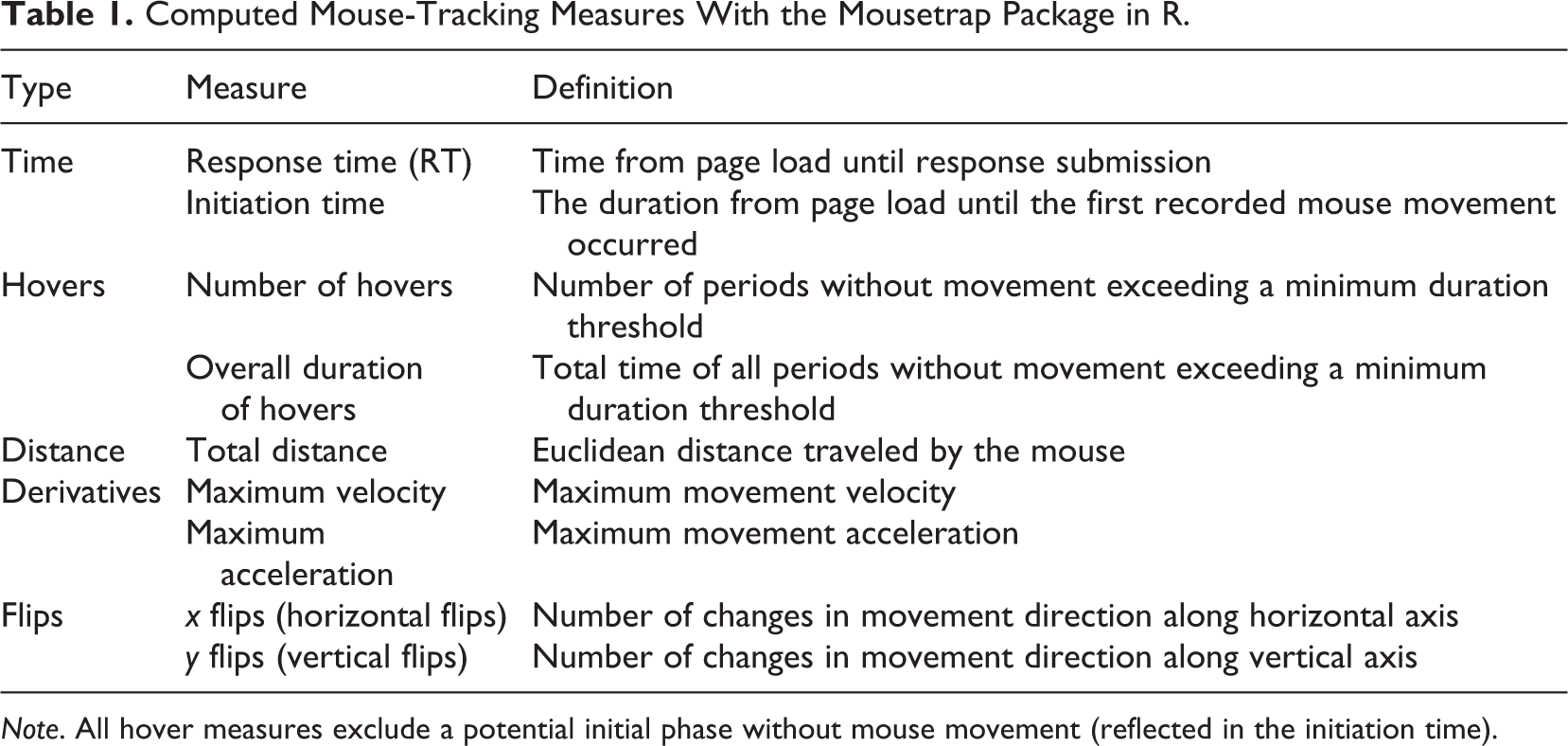
Note. All hover measures exclude a potential initial phase without mouse movement (reflected in the initiation time).

Based on the survey literature summarized above, we hypothesized that several paradata measures could indicate question difficulty, including prolonged response times (Conrad et al., 2007; Mittereder, 2019), longer distances traveled (Stieger & Reips, 2010), and a greater number of hovers and changes in movement direction along the vertical axis (called y flips in Table 1; Horwitz, Kreuter, & Conrad, 2017). We similarly interpret x flips in Table 1 as the number of changes in movement direction along the horizontal axis. However, mouse-tracking applications in the cognitive sciences suggest that multiple measures, including initiation times, velocity, and acceleration, are related to response competition and hence play a role in detecting question difficulty as well (Hehman et al., 2015; Stillman et al., 2018). However, it remains an open question how well all measures together can detect question difficulty, and which are especially useful in a joint analysis.

Classification Supervised Learning Methods

To predict difficulty from mouse movements, we used several common supervised classification methods (Hastie et al., 2009; James et al., 2013). These map a categorical response variable (output or target) to explanatory variables of any type (inputs or predictors) through a specific function (e.g., logit). Our target variable was binary (easy vs. difficult), and we had eleven explanatory variables (mouse-tracking measures as described in Table 1, and age and gender) for each target question. Age and gender were included in all models as predictors because we potentially expected interactions between them and some of the measures (e.g., larger response times may be plausibly associated with older people and thus less indicative for difficulty in this case). These interactions are easily handled by most of the learning methods described below.

Each model is fitted onto a training sample, and its predictive performance evaluated on the remainder of the data set (Hastie et al., 2009; James et al., 2013). To cover different relationships between the outcome and inputs, we considered the following predictive models: logistic regression, tree-based models (classification trees, random forest, and gradient boosting), support vector machines, and single hidden layer back-propagation networks (a kind of neural network).

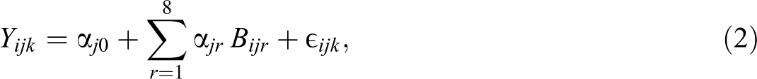
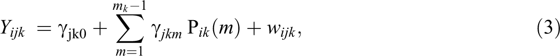
Logistic regression models linearly relate the log odds of the binary outcome Y (here: $Y = 0$ easy, and $Y = 1$ difficult), and the vector of predictors $X = (X_{1}, X_{2}, \dots, X_{p})$ with the equation:

log (odds (Y = 1 | X)) = log (\frac{P (Y = 1 | X)}{1 - P (Y = 1 | X)}) = β_{0} + β_{1} X_{1} + β_{2} X_{2} + . . . + β_{p} X_{p},

where $log (\frac{P (Y = 1 | X)}{1 - P (Y = 1 | X)})$ is the logistic function of $P (Y = 1)$ and acts to linearize the relationship between the output and inputs. The model parameters $β_{1}, . . ., β_{p}$ estimate the relationship between the output and the corresponding input (Hosmer et al., 2013).

Classification trees partition the space of the vector of predictors into a set of different subspaces. This division process is recursive and consists of splitting each predictor at a collection of possible cut points and selecting the partition that most reduces the impurity (e.g., Gini index) within nodes (regions defined by the splits). To control overfitting and reduce tree complexity, these can be pruned, trading a small increase in bias for a larger reduction in variance of predictions. These methods can be unstable in that small variations in the training sample can change the tree structure dramatically (Breiman et al., 1984; Loh, 2014).

Tree-based random forests: Bootstrap aggregating (bagging; Efron & Tibshirani, 1994) draws bootstrap samples from the training data, fitting an unpruned tree to each to ensure minimum bias. Bootstrap trees are then aggregated for a more stable overall prediction (e.g., using the majority vote for class membership). As a high correlation between bootstrap trees diminishes the possible variance reduction in bagging, random forests consider a new random subsample of m predictors (tuning parameter) for each bootstrap tree. This includes weaker predictors in some of the bootstrap trees, increasing variability and decreasing correlation, reducing the variance of the overall prediction. The number of bootstrap trees is also a tuning parameter (see Breiman, 2001; Sutton, 2005).

Tree-based gradient boosting methods were also designed to reduce the trees’ variance and improve the models’ performance. Here, trees are grown sequentially by iteratively fitting a new tree based on the information that was not explained in the previously grown trees (so-called pseudo-residuals, serving as responses in the next iteration). The main tuning parameters are the number of trees and splits in each tree, and a shrinkage parameter that controls how the model learns (see Breiman, 1998; Friedman, 2001).

Support vector machines are used to construct nonlinear decision boundaries to discriminate between different categories. A linear boundary is defined as the hyperplane in the covariate space that gives the largest margin (distance) to the nearest observations (support vectors) in the two classes on both sides of the plane (support vector classifier), while allowing for some misclassifications. As samples are usually not linearly separable into two classes, kernel functions (we considered here the radial kernel) enlarge the predictors’ vector space and ensure that the decision boundary is no longer linear in the original predictors’ vector space. The two tuning parameters are a regularization and a kernel-related (see Cortes & Vapnik, 1995; Steinwart & Christmann, 2008).

Single hidden layer back-propagation networks (a kind of neural networks) consist of inputs, a single hidden layer with h nodes, and outputs that can be represented as a graph. Each node of the hidden layer corresponds to an activation function evaluated at a linear combination of the inputs, where parameters act as weights. The outputs are also nonlinear transformations (e.g., logistic transformations) of linear combinations of these nodes in the hidden layer. The tuning parameters are a regularization and the size of the hidden layer (see Ripley, 1994a, 1994b).

Model Tuning of Parameters, Performance, and Importance Measures

For all models, we assessed predictive performance as the proportion of correct assignments to the two experimental groups (accuracy). We used cross-validation methods for both tuning parameters and evaluating a model’s predictive performance. In cross-validation, the sample is divided into K parts with each part left out in turn as a testing set for the model fitted onto the training set (the remaining K − 1 parts). Parameters are chosen to optimize the average prediction error over the left-out parts. As the parameters are tuned to a given data set, and to get an honest assessment of the out-of-sample prediction error, we used nested cross-validation. Here, for each left-out part of the data (validation set) in the outer loop, cross-validation with further splits of the remaining data into training and test sets is performed (inner loop). While the tuning parameters for each outer fold are chosen using the inner loop, the out-of-sample prediction error of the tuned models is evaluated on the validation sets in the outer loop. This avoids overoptimistic performance evaluation when tuning and validating on the same samples (Varma & Simon, 2006; see also Efron & Tibshirani, 1997; Hastie et al., 2009; James et al., 2013).

We used nested cross-validation for all tuning parameters with 10-fold cross-validation for the outer split and subsampling (500 repetitions) with weights of 75% and 25% for the subtraining and test sets in the inner splits. Since the outcomes are balanced (Wei & Dunbrack, 2013), we used accuracies to evaluate predictive performance in both the inner and outer loops.

All learning models were computed with the mlr package in R 3.6.1 (Bischl et al., 2020) using parallelization with 32 CPUs. Equal training and testing samples were used across the different models for each question to ensure comparability. Results in Tables 2 and 3 are reproducible if the same seeds and number of CPUs are used.

Table 2.

Best Predictive Models and Performance Results for Uncorrected and Corrected Full and Response-Time-Only Models.

Question	Manipulation	Personalization	Model	Supervised Learner	Threshold Hovers (ms)	Accuracy^a	Specificity^b	Sensitivity^c
Employment detail	Concise vs. complex language	No	Full	Classification tree	250^d	.6097	.2951	.8828
		No	Response-time-only	Logit regression		.6171	.6358	.6028
		Baseline	Full	Gradient boosting	2,000	.6587	.5629	.7416
		Baseline	Response-time-only	Classification tree		.6407	.6430	.6376
		Baseline and position	Full	Classification tree	250^d	.6498	.7256	.5772
		Baseline and position	Response-time-only	Classification tree		.6480	.5722	.7065
Employee level	Ordered vs. unordered layout	No	Full	Gradient boosting	3,000	.5548	.4695	.6303
		No	Response-time-only	Gradient boosting		.5569	.4420	.6533
		Baseline	Full	Neural network	3,000	.5670	.7015	.4340
		Baseline	Response-time-only	Classification tree		.5528	.7168	.3919
		Baseline and position	Full	Gradient boosting	3,000	.5909	.5258	.6527
		Baseline and position	Response-time-only	Neural network		.5328	.5498	.5166
Education level		No	Full	Support vector machines	2,000	.5622	.6042	.5204
		No	Response-time-only	Gradient boosting		.5641	.6502	.4783
		Baseline	Full	Neural network	250	.5805	.7053	.4436
		Baseline	Response-time-only	Random forest		.5639	.5489	.5831
		Baseline and position	Full	Random forest	250	.5895	.6233	.5512
		Baseline and position	Response-time-only	Logit regression		.4946	.6117	.4095

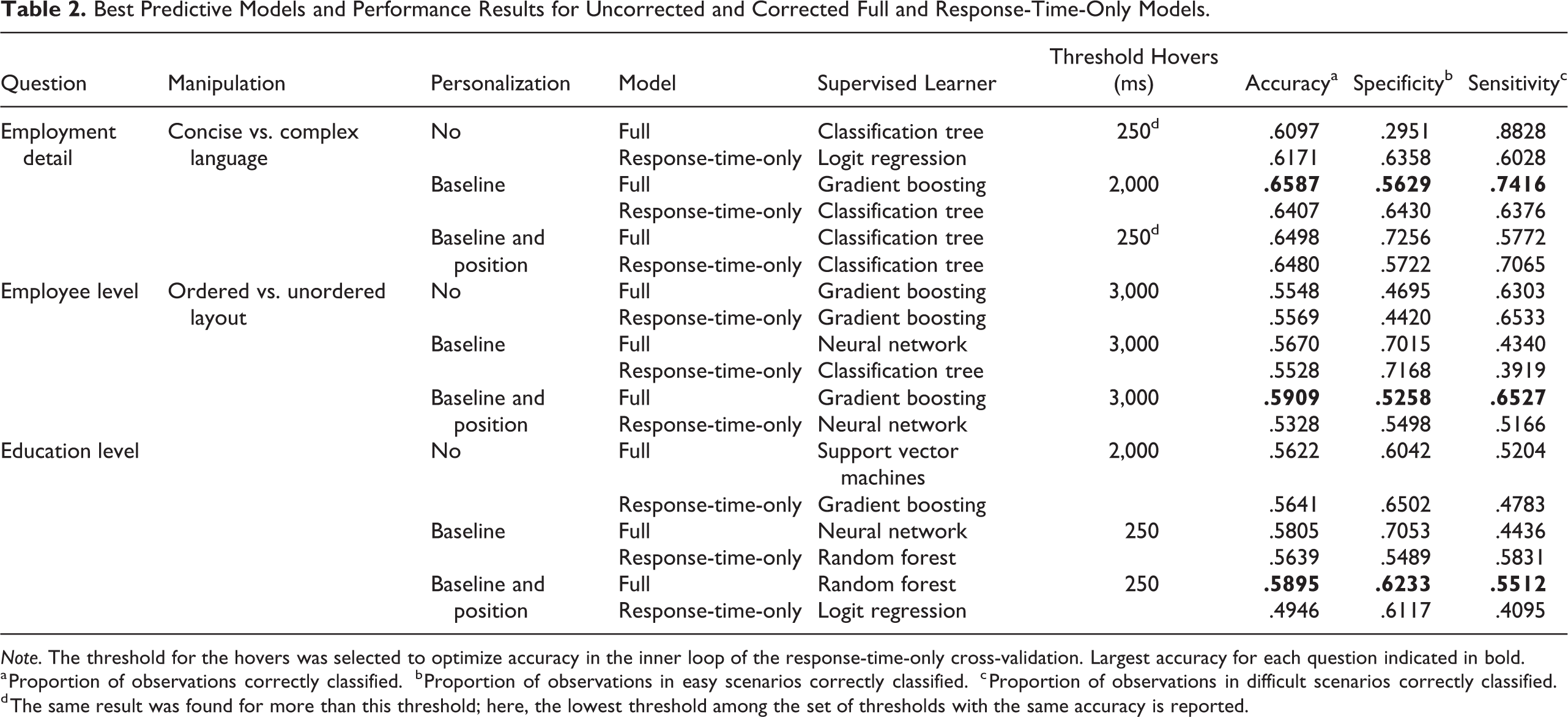
Note. The threshold for the hovers was selected to optimize accuracy in the inner loop of the response-time-only cross-validation. Largest accuracy for each question indicated in bold.

^a Proportion of observations correctly classified.

^b Proportion of observations in easy scenarios correctly classified.

^c Proportion of observations in difficult scenarios correctly classified.

^d The same result was found for more than this threshold; here, the lowest threshold among the set of thresholds with the same accuracy is reported.

Table 3.

Models’ Performance Results for the Best Models and Other Full Model Candidates Who Used the Same Personalization Methods and Thresholds for Hovers as the Corresponding Best Models for Each Target Question.

Question	Manipulation	Personalization	Supervised learner	Accuracy^a	Specificity^b	Sensitivity^c
Employment detail	Concise vs. complex language	Baseline	Logit regression	.6298	.6448	.6169
			Classification Tree	.6189	.5836	.6569
			Random forest	.6134	.5516	.6664
			Gradient boosting	.6587	.5629	.7416
			Support vector machines	.6153	.5755	.6498
			Neural network	.5628	.6866	.4513
Employee level	Ordered vs. unordered layout	Baseline and position	Logit regression	.4751	.3062	.6680
			Classification Tree	.5709	.5275	.6184
			Random forest	.5748	.5286	.6078
			Gradient boosting	.5909	.5258	.6527
			Support vector machines	.5709	.2823	.8435
			Neural network	.5190	.6677	.3780
Education level		Baseline and position	Logit regression	.4820	.5666	.4259
			Classification Tree	.5765	.7013	.4673
			Random forest	.5895	.6233	.5512
			Gradient boosting	.5748	.6683	.4851
			Support vector machines	.4634	.4145	.5644
			Neural network	.5222	.5927	.4249

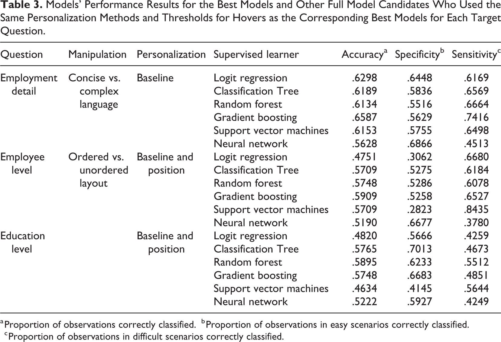
^a Proportion of observations correctly classified.

^b Proportion of observations in easy scenarios correctly classified.

^c Proportion of observations in difficult scenarios correctly classified.

We computed permutational feature importance measures (Strobl et al., 2008) to extract the influence of each predictor in the best-performing models. To do so, we compared the accuracy of the model with a randomly permuted version of the measure (postpermutational accuracy) to the accuracy of the same model with the original measure (prepermutational accuracy). A significant (negative) difference between postpermutational and prepermutational accuracies indicates that the associated measure is important for difficulty prediction. In practice, we averaged the postpermutational accuracy of each measure over 500 models fitted to independently permuted data.

Personalization

We investigated personalization of the measures to reduce variability unrelated to the classification task and correct for different baseline behaviors. Measures may also be influenced by the response, for example, response time or total distance traveled may be larger if the position of the answer is further away from the submit button, but this is unrelated to the question difficulty.

We proposed two methods of personalization: One that only corrects for the baseline behavior of the respondents using the eight nonmanipulated baseline questions, and a second that corrects for the baseline behavior and the position of the chosen answer. This second approach is especially important for manipulations requiring changes in the response choice positions, for example, ordered versus unordered settings, as part of the variability of the measures is only due to the locations of the response choices rather than the difficulty itself, for example, the difficulty locating the correct response choice in the unordered setting. We regressed every measure onto its values in all baseline questions, and on a position indicator for the second correction method, and performed our analyses using the residual values.

To correct for the baseline behavior of the respondents, denote by $B_{i j r}$ the jth measure (e.g., response time) of the ith individual in the rth baseline question (e.g., general economy). Let $Y_{ijk}$ be the jth measure of the ith individual in the kth target question (e.g., employment detail). Consider the following linear regression model:

Y_{i j k} = α_{j 0} + \sum_{r = 1}^{8} α_{j r} B_{i j r} + ϵ_{i j k},

where $α_{jr}$ quantifies the association between the jth measure in the rth baseline and kth target questions, respectively, and $ϵ_{ijk}$ is the part of $Y_{ijk}$ not explained by baseline behaviors. We used the model residuals ${\hat{ϵ}}_{ijk}$ as baseline-corrected measures.

To additionally remove the effect of the position of the responses, we used a two-step method. In the first step, each measure of each target question is corrected for the corresponding positions with the linear regression:

Y_{i j k} = γ_{jk 0} + \sum_{m = 1}^{m_{k} - 1} γ_{j k m} P_{i k} (m) + w_{i j k},

where $P_{i k} (m)$ is an indicator whether the ith individual’s answer in the kth target question was at the mth position (out of m_k options). The residuals from Equation 3, $\hat{w_{i j k}}$ , correspond to the variability of the jth measure in the kth target variable not explained by the response position. Corrected measures $\hat{w_{i j r}}$ for the baseline questions are constructed in the same way.

The second step additionally corrects for the individual characteristics using the linear regression:

\hat{w_{i j k}} = ϕ_{j 0} + ϕ_{j 1} \bar{\hat{w_{i j}}} + v_{i j k},

where $\bar{\hat{w_{i j}}} = \frac{1}{8} \sum_{r = 1}^{8} \hat{w_{i j r}}$ averages over the residuals from Equation 3 within the same individual and the same measure over the eight baseline questions. Finally, the residuals $\hat{v_{i j k}}$ are the position- and baseline-corrected measures.

Results

Target Questions

Employment detail, employee, and education levels had nine, four, and 11 potential response options, respectively. However, only five of the nine response options of employment detail were chosen in our data set. For employee level, all four response alternatives were selected, while, for education level, only eight of the 11 response options were chosen.³

Mouse Movements Measures and Predictive Learning Models

Each of the measures in Table 1 may capture different features of the response process, which might differ between easy and difficult settings. Figure 1 shows the empirical distribution of these measures for both easy and difficult settings for the three target questions. The same figures for baseline-corrected, and baseline and position-corrected measures can be found in the Supplementary Material. These graphs can help identify measures for which the empirical distributions of easy and difficult scenarios are different, and thus, which measures could potentially work best for difficulty prediction. However, differences between distributions (e.g., median) of a particular measure for easy and difficult scenarios do not directly guarantee that this specific measure will predict difficulty well.

Figure 1.

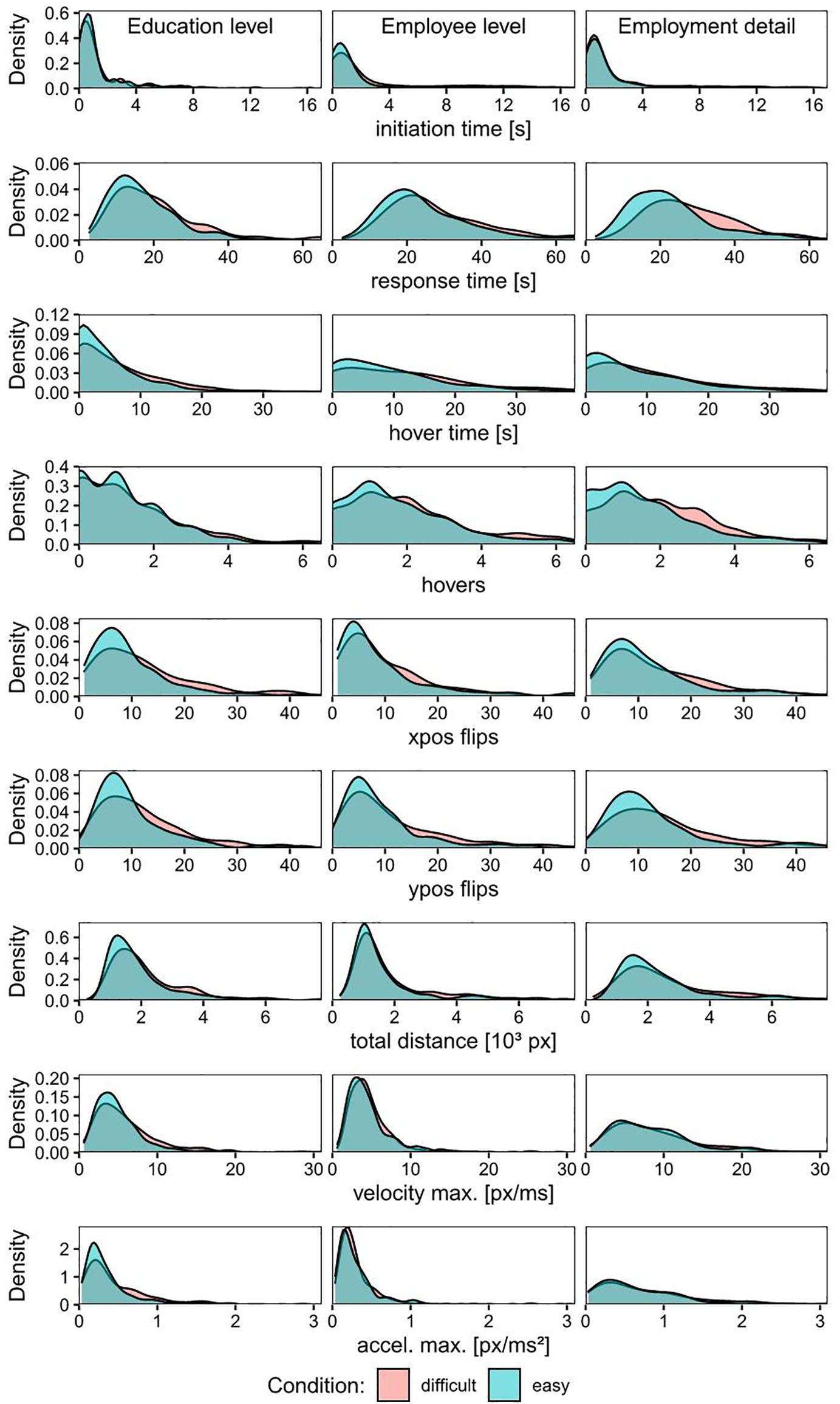
Empirical distribution of the uncorrected measures separately for each target question (education and employee levels, and employment detail from left to right) and difficulty condition (blue = easy, red = difficult). Note. The smoothed kernel density estimates are presented. Axis limits are set, so that for each question and measure, >95% of the values are displayed.

For each target question, each predictive model described above was considered as a potential classifier using the experimental condition (easy or difficult) as a target variable, and the measures in Table 1, and age and gender as predictors. When personalization was also considered, the measures in Table 1 were corrected before being included as predictors.

Table 2 shows the best learning models among all candidates, in terms of accuracy, for each target question and personalization approach. This table compares the best model found when using nonpersonalized and personalized measures and considering either response-time-only or response time and other measures as predictors to investigate the gain in accuracy or added value of the extracted mouse-tracking measures over just response time for different kinds of difficulty. Both the full model with all nine measures and the response-time-only version also included age and gender as predictors, as we potentially expected interactions between some measures and these demographic covariates. More details on the full results for each model and question, and the corresponding R codes, are in the Supplementary Material (Tables S2, S3, and S4).

Hover-type measures are computed depending on a threshold that is usually chosen empirically. Horwitz, Kreuter, and Conrad (2017) considered 2,000 ms as a threshold for hovers. To investigate dependence on this parameter, we conducted an extensive study considering the following thresholds: 250 ms, 500 ms, 2,000 ms, and 3,000 ms. As shown in Table 2, no threshold was uniquely optimal for all questions, and results were similar across thresholds in many cases.

For employment detail, gradient boosting with age, gender, and nine baseline-corrected measures (full model) performed best among the predictive models. On average, this model correctly classified 65.9% of the observations (accuracy); in particular, the proportions of easy and difficult scenarios correctly classified (i.e., specificity and sensitivity) were 56.3% and 74.2%, respectively. The best full model with uncorrected measures only provided an accuracy of 61.0%, indicating the necessity for personalization. The best response-time-only model showed an accuracy of 64.8%, a bit lower than the accuracy of the best model, indicating a small gain of using all mouse-tracking measures over the response-time-only model. All these three models give accuracies around 64%–65%, and thus over the 50% expected in a coin-toss experiment, although there is still room for improvement.

Figure 2 shows the impact of each measure on each target question’s best-performing learning model’s predictive performance as measured by the “permutation feature importance” with the reduction in accuracy when permuting a given feature for each target question and measure (cf. description in Model Tuning of Parameters, Performance and Importance Measures section). The larger the difference, the more impact the measure has in the model. For employment detail (green points), the most important measures in this gradient boosting were response time, and the number of y flips and x flips with an average decrease in the model’s accuracy of 0.142, 0.028, and 0.014, respectively.

Figure 2.

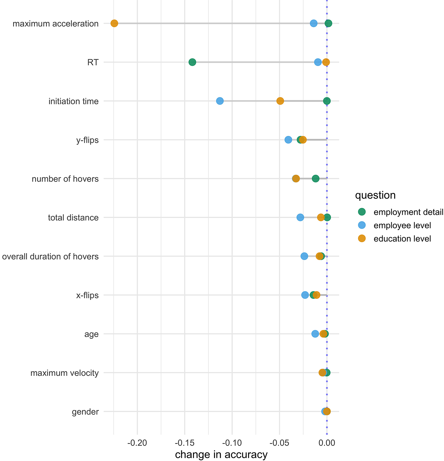
Measures’ importance based on permutation methods (cf. see Model Tuning of Parameters, Performance, and Importance Measures section). Note. The best learning models for employment detail and employee level (gradient boosting) and education level (random forest) are used to compute both the postpermutational and prepermutational accuracies. Green (employment detail), blue (employee level), and yellow (education level) points represent the differences between the respective postpermutational and prepermutational accuracies based on these learning models. The more negative the change in accuracy, the more impact has the measure in the respective model.

For employee level, gradient boosting with all baseline- and position-corrected measures as predictors again performed best in terms of accuracy. Overall, 59.1% of the observations (i.e., accuracy), and 52.6% and 65.3% (i.e., specificity and sensitivity) of the easy and difficult scenarios were classified correctly. The best full model for the uncorrected measures and the best response-time-only model showed accuracies of 55.5% and 55.7%, respectively, both again smaller than that of the overall best model. The best learning model for this specific target question showed an accuracy around 59%, which is above the threshold of 50% expected in a coin-toss-based model. If we do not personalize measures and/or only use response time as a predictor of difficulty in this question, the best accuracies, given the predictive models we use, are usually around 55%, and thus closer to a coin-toss-based model. Figure 2 (blue points) shows that the most important measures in the gradient boosting for employee level were initiation time, x flips, and hovers with an average decrease in the model’s overall accuracy of 0.113, 0.041, and 0.033, respectively. However, for this particular question, permuting response time decreased the overall accuracy by only 0.009, indicating the necessity of more measures to predict the difficulty in the corresponding manipulation.

For education level, a random forest with 11 baseline- and position-corrected measures performed best in terms of accuracy. This model correctly classified 58.9% (i.e., accuracy) of the observations, with easy and difficult scenarios correctly classified with rates of 62.3% and 55.1% (i.e., specificity and sensitivity), respectively. The best full model for the uncorrected measures and the best response-time-only model only showed accuracies of 56.2% and 56.4%, respectively, decreasing accuracy closer to the 50% of a coin flip compared to the best model based on all personalized measures. Figure 2 (yellow points) shows that the most important measures in the random forest were maximum acceleration, initiation time, and hovers with an average accuracy decrease when permuted of 0.224, 0.049, and 0.033, respectively. For this question again, randomly permuting response time did not decrease the overall accuracy notably.

Overall, we found that for all three target questions, inclusion of all measures improved accuracy compared to the response-time-only models, indicating that mouse movements contain more information about the presence of a suboptimally phrased item than the response time alone. A stronger gain in accuracy was evident when personalizing the measures, indicating the importance of considering different respondents’ habitual behaviors. Considering the position of the answer category was additionally beneficial if the answers were differently ordered. We also found that while there were significant differences in measures between easy and difficult settings, the manipulations were not strong enough to allow for reliable prediction of difficulty from the measures alone. Finally, it seemed that tree-based models generally work better than non-tree-based models in our data, and their accuracies for all three target questions are roughly between 59% and 65%, well above 50%. In particular, Table 3 compares the best model for each question (Table 2) to the other considered predictive models within the personalization method that works best in each case. For both employee and education levels, the best accuracies and the accuracies of the other tree-based models differed by roughly 0.012 and 0.015, respectively. Bigger raw differences of 0.12, 0.02, and 0.07, and 0.11, 0.13, and 0.07 were observed between the best accuracies and the accuracies of the logistic regression, support vector machine, and neural network models for employee and education levels, respectively. For employment detail, raw differences between the best accuracies and the accuracies of tree- and non-tree-based models were generally smaller, except for the worse performing neural networks. However, the performance of tree-based models was still satisfactory and included the best model.

For our application, we used a relatively wide range of methods that differ in several aspects, which may explain why some do better than others. For example, the logistic regression is less flexible than other methods as it linearly relates the log odds of the response (e.g., difficulty) and the predictors (e.g., measures). Thus, such a regression is not appropriate if the linearity is violated. The comparatively worse performance of the logistic regression compared to machine learning methods in our case seems to indicate that linearity does not hold here, and more complex models are necessary. Tree-based models, however, are more versatile as they can accommodate more complex relationships between the response and predictors and even consider multiple interactions between different predictors (e.g., age and response time). Also, ensemble methods (gradient boosting and random forest) often improve weaker learning models’ predictive capabilities (e.g., classification trees) because they can reduce their variance and bias. For our data and types of difficulty, it seemed that these models have captured the relationships between response and predictors in an improved manner. Finally, both support vector machines and neural networks also fit more complex relationships between response and predictors than logistic regression. We have here defined decision boundaries based on radial kernels for support vector machines, and we have used the simplest form of neural networks with only one hidden layer. It may be possible to improve their performance by investigating additional kernels or additional hidden layers.

To summarize, we found here that tree-based models, particularly random forest and gradient boosting, are the predictive models that best capture the relationships between the response and measures. When personalization is further considered, both random forest and gradient boosting improve considerably. Therefore, such models with between-individual adjusted measures seem to be a promising method for detecting difficulty in survey questions with characteristics comparable to those investigated in the current paper’s target questions.

Discussion

This work aimed to predict the presence of problems with particular items in a web survey based on measures commonly used in cognitive science and, more recently, the survey literature. We found that the use of several measures improved the prediction of question difficulty, above and beyond the use of response times. We also saw that further improvements in prediction were achievable by controlling for between-participant differences in the measures with baseline questions.

Question difficulty causes measurement error in web surveys and can lead to poor data quality and potentially weaken or bias results and conclusions. The detection of such difficulty is an important step in identifying items with potential for improvement, developing corrections for measurement error when analyzing survey responses and potentially even implementing real-time interventions while participants fill out a survey. Real-time interventions could stretch from pop-up help screens (Mittereder, 2019), reminders to respond carefully (Conrad et al., 2017), all the way to chat assistance, either by a bot or a human. To both do not miss an unnecessarily difficult item while at the same time not to bother a respondent unnecessarily with such interventions, the good performance of any predictive model triggering the intervention is key. Because mouse-tracking is an unobtrusive data collection mode, practitioners might consider gathering interaction data by default, and sharing measures of difficulty derived from paradata alongside the collected responses so that other users of the data can screen for difficulties, even if they do not analyze the paradata themselves.

For our three target questions, we found that the best predictive models were tree-based models (particularly random forest and gradient boosting) that use baseline- or, if the position differs by experimental conditions within the same questions, position- and baseline-corrected measures and that response time was not always the most important measure for predicting difficulty. Particularly, response time was the most relevant measure in the best predictive model for employment detail (easy vs. difficult language). However, measures such as initiation time, maximum acceleration, x flips, and hovers improved difficulty prediction more than response time for both employee and education levels (ordered vs. randomly ordered response options). This might indicate that different manipulations produced different types of difficulty, which can be captured through different paradata sources. Also, the most important features differed by question even if these were manipulated in the same manner, and difficulty was potentially similar. For example, maximum acceleration was the most important measure for education level but not useful for employee-level difficulty prediction. This could be explained by the fact that the number of response options was larger for the education-level question and that participants in the unordered condition for this question might have more often and more strongly shown variations in their cursor speed.

The best learning models found here are based on a data set limited to mouse users who made up the majority of respondents in our study. While similar predictive models as ours could in general also be developed for other input devices, such extensions would need to develop corresponding summary measures similarly to the measures used here, and their use remains to be tested empirically.

Even when using a large set of mouse-tracking measures and accounting for individual variability, there is still room for improvements when predicting response difficulty, given that our best learning models showed only moderately high accuracies (i.e., roughly between 59% and 65%). Some explanations on why we cannot correctly classify in a higher range could be related to the (low) intensity of the manipulations. Although questions were experimentally manipulated to create two controlled difficulty levels, manipulations each changed only a very specific aspect of the item, which may not have caused strong difficulties in answering for all respondents. As we did not collect subjective difficulty ratings, we cannot quantify the level of difficulty participants perceived nor the magnitude of difference between conditions. Hence, the average degree of response difficulty might not have varied very strongly between conditions. Also, the strength of these manipulations may not have been comparable for all participants and questions, and we might thus have observed a mixture of behaviors, with some participants in the difficult setting not experiencing subjective difficulty. Since the different difficulty manipulations were varied between questions, we cannot disentangle effects of the specific question from effects of the type of difficulty, for example, on the most relevant feature. These might be some of the reasons why our accuracies are only moderately high. A complementary approach could measure participants’ subjective difficulty for a given question and use it as the outcome for prediction (Horwitz, Kreuter, & Conrad, 2017). Also, future research could include additional difficulty manipulations or manipulate different types of difficulty within the same question in a crossed design. Similarly, to further elucidate the cognitive processes that might have led to any particular response and paradata trace, practitioners might consider using cognitive interviewing or probing to elicit a subjective recollection of the response process (e.g., Beatty & Willis, 2007; Behr et al., 2012).

Another explanation for the limited classification performance might be that measures only use summaries of the information in the mouse movements. Future research may consider the use of full mouse movement trajectories, if suitable functional data methods are developed. Also, the information from mouse movements could in a future study be enriched by additional information such as respondents’ click data and changes in the response options. Finally, we also plan to use linked administrative data that allow us to quantify measurement error in certain survey responses and investigate an analogous prediction of measurement error.

Supplementary Material

Supplemental Material, sj-pdf-1-ssc-10.1177_08944393211032950 - Predicting Question Difficulty in Web Surveys: A Machine Learning Approach Based on Mouse Movement Features

Supplemental Material, sj-pdf-1-ssc-10.1177_08944393211032950 for Predicting Question Difficulty in Web Surveys: A Machine Learning Approach Based on Mouse Movement Features by Amanda Fernández-Fontelo, Pascal J. Kieslich, Felix Henninger, Frauke Kreuter and Sonja Greven in Social Science Computer Review

Supplementary Material

Supplemental Material, sj-pdf-2-ssc-10.1177_08944393211032950 - Predicting Question Difficulty in Web Surveys: A Machine Learning Approach Based on Mouse Movement Features

Supplemental Material, sj-pdf-2-ssc-10.1177_08944393211032950 for Predicting Question Difficulty in Web Surveys: A Machine Learning Approach Based on Mouse Movement Features by Amanda Fernández-Fontelo, Pascal J. Kieslich, Felix Henninger, Frauke Kreuter and Sonja Greven in Social Science Computer Review

Footnotes

Acknowledgments

The authors thank the Institute for Employment Research (IAB) for their support in conducting the survey that provided the data for our analyses, and particularly Malte Schierholz and Ursula Jaenichen for providing guidance and insights into the data. Also, the authors thank student assistants Anja Humbs, Zhang Ran and Franziska Leipold for their help in setting up the original survey, running the analyses and with the reference management.

Data Availability

Our data are available at the Institute for Employment Research:

Declaration of Conflicting Interests

The authors declared no potential conflicts of interest with respect to the research, authorship, and/or publication of this article.

Funding

The authors disclosed receipt of the following financial support for the research, authorship, and/or publication of this article: The authors acknowledge financial support from the German Research Foundation (DFG) through the grant “Statistical modeling using mouse movements to model measurement error and improve data quality in web surveys” (GR 3793/2 -1 and KR 2211/5 -1).

Supplementary Material

The supplementary materials and R codes are available at

Notes

References

Beatty

P. C.

Willis

G. B.

(2007). Research synthesis: The practice of cognitive interviewing. Public Opinion Quarterly, 71(2), 287–311. https://doi.org/10.1093/poq/nfm006

Behr

Kaczmirek

Bandilla

Braun

(2012). Asking probing questions in web surveys: Which factors have an impact on the quality of responses? Social Science Computer Review, 30(4), 487–498. https://doi.org/10.1177/0894439311435305

Bischl

Lang

Kotthoff

Schiffner

Richter

Jones

Casalicchio

Gallo

Schratz

Bossek

Studerus

Judt

Kuehn

Kerschke

Fendt

Probst

Sun

Thomas

Vieira

… Spooner

. (2020). mlr: Machine learning in R (Version 2.17.0) [Computer software]. https://CRAN.R-project.org/package=mlr

Breiman

(1998). Arcing classifier (with discussion and a rejoinder by the author). The Annals of Statistics, 26(3), 801–849. https://doi.org/10.1214/aos/1024691079

Breiman

(2001). Random forests. Machine Learning, 45(1), 5–32. https://doi.org/10.1023/A:1010933404324

Breiman

Friedman

Stone

C. J.

Olshen

R. A.

(1984). Classification and regression trees. Taylor & Francis Group. https://doi.org/10.1201/9781315139470

Callegaro

(2013). Paradata in web surveys. In Kreuter

(Ed.), Improving surveys with paradata: Analytic uses of process information (pp. 263–282). John Wiley & Sons. https://doi.org/10.1002/9781118596869ch11

Chun

A. Y.

Schouten

Wagner

(2017). JOS special issue on responsive and adaptive survey design: Looking back to see forward – editorial. Journal of Official Statistics, 33(3), 571–577. https://doi.org/10.1515/jos-2017-0027

Conrad

F. G.

Couper

M. P.

Tourangeau

Peytchev

(2006). Use and non-use of clarification features in web surveys. Journal of Official Statistics, 22(2), 245–269.

10.

Conrad

F. G.

Couper

M. P.

Tourangeau

Zhang

(2017). Reducing speeding in web surveys by providing immediate feedback. Survey Research Methods, 11(1), 45–61. https://doi.org/10.18148/srm/2017.v11i1.6304

11.

Conrad

F. G.

Schober

M. F.

Coiner

(2007). Bringing features of human dialogue to web surveys. Applied Cognitive Psychology, 21(2), 165–187. https://doi.org/10.1002/acp.1335

12.

Conrad

F.G.

Schober

M.F.

(2000). Clarifying question meaning in a household telephone survey. Public Opinion Quarterly, 64, 1–28. https://doi.org/10.1086/316757

13.

Cortes

Vapnik

(1995). Support-vector networks. Machine Learning, 20(3), 273–297. https://doi.org/10.1007/BF00994018

14.

Couper

M. P.

(2011). The future of modes of data collection. Public Opinion Quarterly, 75(5), 889–908.

15.

Couper

M. P.

Kreuter

(2013). Using paradata to explore item level response times in surveys. Journal of the Royal Statistical Society: Series A (Statistics in Society), 176(1), 271–286. https://doi.org/10.1111/j.1467-985X.2012.01041.x

16.

de Leeuw

E. D.

(2005). To mix or not to mix data collection modes in surveys. Journal of Official Statistics, 21(2), 233–255.

17.

Early

(2017). Dynamic question ordering: Obtaining useful information while reducing user burden. Carnegie Mellon University.

18.

Efron

Tibshirani

(1997). Improvements on cross validation: The .632+ bootstrap method. Journal of the American Statistical Association, 92(438), 548–560. https://doi.org/10.2307/2965703

19.

Efron

Tibshirani

R. J.

(1994). An introduction to the bootstrap. CRC Press.

20.

Ehlen

Schober

M.F.

Conrad

F.G.

(2007). Modeling speech disfluency to predict conceptual misalignment in speech survey interfaces. Discourse Processes, 44 (3): 245–265. https://doi.org/10.1080/01638530701600839

21.

Freeman

J. B.

(2018). Doing psychological science by hand. Current Directions in Psychological Science. https://doi.org/10.1177/0963721417746793

22.

Freeman

J. B.

Ambady

(2011). A dynamic interactive theory of person construal. Psychological Review, 118(2), 247–279. https://doi.org/10.1037/a0022327

23.

Friedman

J. H.

(2001). Greedy function approximation: A gradient boosting machine. The Annals of Statistics, 29(5), 1189–1232. https://doi.org/10.1214/aos/1013203451

24.

Groves

R. M.

Fowler

F. J.

Jr Couper

M. P.

Lepkowski

J. M.

Singer

Tourangeau

(2009). Survey methodology. Wiley.

25.

Hastie

Tibshirani

Friedman

. (2009). The elements of statistical learning: Data mining, inference, and prediction (2nd ed.). Springer-Verlag. https://doi.org/10.1007/978-0-387-84858-7

26.

Heerwegh

(2003). Explaining response latencies and changing answers using client-side paradata from a web survey. Social Science Computer Review, 21(3), 360–373. https://doi.org/10.1177/0894439303253985

27.

Hehman

Stolier

R. M.

Freeman

J. B.

(2015). Advanced mouse-tracking analytic techniques for enhancing psychological science. Group Processes & Intergroup Relations, 18(3), 384–401. https://doi.org/10.1177/1368430214538325

28.

Henninger

Kieslich

P. J

. (2020). Mousetrap-web:Mouse-tracking for the browser [Manuscript submitted for publication].

29.

Höhne

J. K.

Schlosser

(2018). Investigating the adequacy of response time outlier definitions in computer-based web surveys using paradata SurveyFocus. Social Science Computer Review, 36(3), 369–378. https://doi.org/10.1177/0894439317710450

30.

Holbrook

Cho

Y. I.

Johnson

(2006). The impact of question and respondent characteristics on comprehension and mapping difficulties. Public Opinion Quarterly, 70(4), 565–595. https://doi.org/10.1093/poq/nfl027

31.

Horwitz

Brockhaus

Henninger

Kieslich

P. J.

Schierholz

Keusch

Kreuter

(2017). Learning from mouse movements: Improving questionnaire and respondents’ user experience through passive data collection [IAB discussion paper, No. 34/2017]. Institut für Arbeitsmarkt- und Berufsforschung (IAB), Nürnberg. http://doku.iab.de/discussionpapers/2017/dp3417.pdf

32.

Horwitz

Brockhaus

Henninger

Kieslich

P. J.

Schierholz

Keusch

Kreuter

(2019). Learning from mouse movements: Improving questionnaire and respondents’ user experience through passive data collection. In Bearry

P. C.

Wilmot

Collins

Kaye

Padilla

J. L.

Willis

(Eds.), Advances in questionnaire design, development, evaluation and testing (pp. 403–426). Wiley. https://doi.org/10.1002/9781119263685.ch16

33.

Horwitz

Kreuter

Conrad

(2017). Using mouse movements to predict web survey response difficulty. Social Science Computer Review, 35(3), 388–405. https://doi.org/10.1177/0894439315626360

34.

Hosmer

D. W.

Lemeshow

Sturdivant

R. X.

(2013). Applied logistic regression (3rd ed.). Wiley.

35.

James

Witten

Hastie

Tibshirani

. (2013). An introduction to statistical learning: With applications in R. Springer-Verlag. https://doi.org/10.1007/978-1-4614-7138-7

36.

Kieslich

P. J.

Henninger

Wulff

D. U.

Haslbeck

J. M. B.

Schulte-Mecklenbeck

(2019). Mouse-tracking: A practical guide to implementation and analysis. In Schulte-Mecklenbeck

Kühberger

Johnson

J. G.

(Eds.), A handbook of process tracing methods (pp. 111–130). Routledge. https://doi.org/10.31234/osf.io/zuvqa

37.

Kreuter

. (Ed.). (2013). Improving surveys with paradata (1st ed.). John Wiley & Sons. https://doi.org/10.1002/9781118596869

38.

Leiner

D. J

. (2014). SoSci survey (2.6.00-i) [Computer software]. https://www.soscisurvey.de

39.

Lenzner

Kaczmirek

Lenzner

(2010). Cognitive burden of survey questions and response times: A psycholinguistic experiment. Applied Cognitive Psychology, 24(7), 1003–1020. https://doi.org/10.1002/acp.1602

40.

Chernoff

Zheng

S.-H.

(2015). Why significant variables aren’t automatically good predictors. Proceedings of the National Academy of Sciences, 112(45), 13892–13897. https://doi.org/10.1073/pnas.1518285112

41.

Loh

W.-Y.

(2014). Fifty years of classification and regression trees. International Statistical Review, 82(3), 329–348. https://doi.org/10.1111/insr.12016

42.

Lord

F. M.

Novick

M. R.

(1968). Statistical theories of mental test scores. Addison-Wesley, Menlo Park.

43.

Mayerl

Sellke

Urban

(2005). Analyzing cognitive processes in CATI surveys with response latencies: An empirical evaluation of the consequences of using different baseline speed measures. Schriftenreihe des Instituts für Sozialwissenschaften der Universität Stuttgart -SISS, Stuttgart. https://doi.org/10.18419/opus-5466

44.

McClain

C. A.

Couper

M. P.

Hupp

A. L.

Keusch

Peterson

Piskorowski

A. D.

West

B. T.

(2019). A typology of web survey paradata for assessing total survey error. Social Science Computer Review, 37(2), 196–213. https://doi.org/10.1177/0894439318759670

45.

Mittereder

F. K.

(2019). Predicting and preventing break off in web surveys. University of Michigan.

46.

O’Hora

Carey

Kervick

Crowley

Dabrowski

(2016). Decisions in motion: Decision dynamics during intertemporal choice reflect subjective evaluation of delayed rewards. Scientific Reports, 6(1), 1–17. https://doi.org/10.1038/srep20740

47.

Olson

(2012). Paradata for nonresponse adjustment. The Annals of the American Academy of Political and Social Science, 645(1), 142–170. https://doi.org/10.1177/0002716212459475

48.

Presser

Couper

M. P.

Lessler

J. T.

Martin

Rothgeb

J. M.

Singer

(2004). Methods for testing and evaluating survey questions. Public Opinion Quarterly, 68(1), 109–130. https://doi.org/10.1093/poq/nfh008

49.

Ripley

B. D.

(1994a). Neural networks and flexible regression and discrimination. Journal of Applied Statistics, 21(1–2), 39–57. https://doi.org/10.1080/757582967

50.

Ripley

B. D.

(1994b). Neural networks and related methods for classification. Journal of the Royal Statistical Society. Series B (Methodological), 56(3), 409–456. https://doi.org/10.1111/j.2517-6161.1994.tb01990.x

51.

Sakshaug

J. W.

Schmucker

Kreuter

Couper

M. P.

Singer

(2016). Evaluating active (opt-in) and passive (opt-out) consent bias in the transfer of federal contact data to a third-party survey agency. Journal of Survey Statistics and Methodology, 4(3), 382–416. https://doi.org/10.1093/jssam/smw020

52.

Schober

M. F.

Conrad

F. G.

Dijkstra

Ongena

Y. P

. (2012). Disfluencies and gaze aversion in unreliable responses to survey questions. Journal of Official Statistics, 28(4), 555–582.

53.

Schober

M. F.

Conrad

F. G.

Fricker

S. S.

(2004). Misunderstanding standardized language in research interviews. Applied Cognition Psychological. 18, 169–188. https://doi.org/10.1002/acp.955

54.

Sendelbah

Vehovar

Slavec

Petrovčič

(2016). Investigating respondent multitasking in web surveys using paradata. Computers in Human Behavior, 55, 777–787. https://doi.org/10.1016/j.chb.2015.10.028

55.

Sharma

S. N.

(2019). Paradata, interviewing quality, and interviewer effects. University of Michigan.

56.

Shmueli

(2010). To explain or to predict? Statistical Science, 25(3), 289–310. https://doi.org/10.1214/10-STS330

57.

Steinwart

Christmann

. (2008). Support vector machines. Springer-Verlag. https://doi.org/10.1007/978-0-387-77242-4

58.

Stern

M. J.

(2008). The use of client-side paradata in analyzing the effects of visual layout on changing responses in web surveys. Field Methods, 20(4), 377–398. https://doi.org/10.1177/1525822X08320421

59.

Stieger

Reips

U.-D.

(2010). What are participants doing while filling in an online questionnaire: A paradata collection tool and an empirical study. Computers in Human Behavior, 26(6), 1488–1495. https://doi.org/10.1016/j.chb.2010.05.013

60.

Stillman

P. E.

Medvedev

Ferguson

M. J.

(2017). Resisting temptation: Tracking how self-control conflicts are successfully resolved in real time. Psychological Science, 28(9), 1240–1258. https://doi.org/10.1177/0956797617705386

61.

Stillman

P. E.

Shen

Ferguson

M. J.

(2018). How mouse-tracking can advance social cognitive theory. Trends in Cognitive Sciences, 22(6), 531–543. https://doi.org/10.1016/j.tics.2018.03.012

62.

Strobl

Boulesteix

A.-L.

Kneib

Augustin

Zeileis

(2008). Conditional variable importance for random forests. BMC Bioinformatics, 9(1), 307. https://doi.org/10.1186/1471-2105-9-307

63.

Sutton

C. D

. (2005). Classification and regression trees, bagging, and boosting. In Rao

C. R.

Wegman

E. J.

Solka

J. L.

(Eds.), Handbook of statistics: data mining and data visualization (Vol. 24). Elsevier. https://doi.org/10.1016/S0169-7161(04)24011-1

64.

Tourangeau

Conrad

F. G.

Couper

M. P

. (2013). The science of web surveys. Oxford University Press. https://doi.org/10.1093/acprof:oso/9780199747047.001.0001

65.

Tourangeau

Rips

L. J.

Rasinski

. (2000). The psychology of survey response. Cambridge University Press. https://doi.org/10.1017/CBO9780511819322

66.

U.S. Census Bureau (2017). Annual report of the center for statistical research and methodology: Fiscal year 2017. Center for Statistical Research and Methodology. https://www.census.gov/content/dam/Census/library/publications/2017/adrm/2017-CSRM-Annual-Report.pdf

67.

Vandenplas

Loosveldt

Beullens

(2017). Fieldwork monitoring for the European social survey: An illustration with Belgium and the Czech Republic in round 7. Journal of Official Statistics, 33(3), 659–686. https://doi.org/10.1515/jos-2017-0031

68.

Varma

Simon

(2006). Bias in error estimation when using cross-validation for model selection. BMC Bioinformatics, 7, 91. https://doi.org/10.1186/1471-2105-7-91

69.

Wei

Dunbrack

R. L.

(2013). The role of balanced training and testing data sets for binary classifiers in bioinformatics. PLoS One, 8(7). https://doi.org/10.1371/journal.pone.0067863

70.

Yan

Olson

(2013). Analyzing paradata to investigate measurement error. In Kreuter

(Ed.), Improving surveys with paradata (pp. 73–95). John Wiley & Sons. https://doi.org/10.1002/9781118596869ch4

71.

Yan

Ryan

Becker

S. E.

Smith

(2015). Assessing quality of answers to a global subjective well-being question through response times. Survey Research Methods, 9(2), 101–109.

72.

Yan

Tourangeau

(2008). Fast times and easy questions: The effects of age, experience and question complexity on web survey response times. Applied Cognitive Psychology, 22(1), 51–68. https://doi.org/10.1002/acp.1331

73.

Yarkoni

Westfall

(2017). Choosing prediction over explanation in psychology: Lessons from machine learning. Perspectives on Psychological Science, 12(6), 1100–1122. https://doi.org/10.1177/1745691617693393

74.

Zhang

Conrad

(2014). Speeding in web surveys: The tendency to answer very fast and its association with straightlining. Survey Research Methods, 8(2), 127–135. https://doi.org/10.18148/srm/2014.v8i2.5453

Supplementary Material

Please find the following supplemental material available below.

For Open Access articles published under a Creative Commons License, all supplemental material carries the same license as the article it is associated with.

For non-Open Access articles published, all supplemental material carries a non-exclusive license, and permission requests for re-use of supplemental material or any part of supplemental material shall be sent directly to the copyright owner as specified in the copyright notice associated with the article.

0.00 MB

1.04 MB

1.99 MB