
Abstract
Combining data from a sample survey, the 2013 Oxford Internet Survey, with the 2011 UK Census, we employ small area estimation to estimate Internet use in small geographies in Britain. This is the first attempt to estimate Internet use at any small-scale level. Doing so allows us to understand the local geographies of British Internet use, showing that the area with least use is in the North East, followed by central Wales. The highest Internet use is in London and southeastern England. The most interesting finding is that after controlling for demographic variables, geographic differences become nonsignificant. The apparent geographic differences appear to be due to differences in demographic characteristics. We conclude by considering the policy implications of this fact.
The Internet has fundamentally reorganized economic, social, and political actions and relationships around the world. It has sparked what has been dubbed as an “information revolution” and given rise to an “information economy” and “information society.” An unimaginable amount of content can now be accessed from almost anywhere on the planet: content that ultimately shapes our understandings of the world and the ways in which we interact with our surroundings. Social life is increasingly mediated, influenced, and augmented by online interactions that take place through the Internet (Graham, Zook, & Boulton, 2013).
Yet despite the importance of the Internet in everyday life, we know surprisingly little about the geography of Internet use and participation at subnational scales. It is unclear whether citizens of Aberdeen, Manchester, Cardiff, or London are significantly more likely to be able to access our global network. This is important because, as we discuss below, there are widespread geographic differences in online activity. Because the differences may indicate digital inequalities on a geographic level, it is important to investigate further. As a result, this article proposes a novel method to calculate the local geographies of Internet usage. In this article, we employ Britain as a case study but, in future work, hope to be able to replicate the method in other parts of the world.
Britain has one of the largest Internet economies in the developed world. The Internet contributes an estimated 8.3% to Britain’s gross domestic product (GDP) (Dean et al., 2012), a share of the economy that is larger than health care, construction, or education. Furthermore, researchers at the Boston Consulting Group predict the Internet’s share of Britain’s economy will grow at a rate of 11% per year over the next 4 years (Dean et al., 2012). This is a faster growth rate than China’s digital economy and more than double the growth rate of the United States. The increasing embeddedness of the Internet in the British economy potentially provides a range of tangible benefits. The Internet strongly supports domestic job and income growth by reducing a range of geographic frictions and allowing access to new customers, sales channels, markets, and ideas. Shortening supply chains and online efficiencies produce lower prices online, saving an estimated £18 billion per year in 2009 (Kalapesi, Willersdorf, & Zwillenberg, 2010). People benefit from better communications, giving them more contact with friends, and better access to jobs. Businesses are more likely to locate in areas with good digital access, thereby boosting local economies and providing jobs that reduce unemployment (Malecki & Moriset, 2008).
In addition to benefits to the UK as a whole, there are personal benefits to Internet use. These benefits include lower prices, access to wider and cheaper entertainment, better and easier access to information, superior access to news, capability to publish your own thoughts to a (potentially large) audience, and—above all—cheaper, easier, faster communication of all kinds. The advantages of the Internet are denied to people who are not online. 1 This has led to a stream of research on people who are not online. The initial work (e.g., Katz & Aspden, 1997; Hoffman & Novak, 1998; van Dijk, 2006) focused on who did or did not have physical access in the form of a computer and an Internet link. Work on this first-level digital divide led to the recognition that Internet access was not enough. There were differences in how effectively people were able to take advantage of the benefits of the Internet (DiMaggio, Hargittai, Celeste, & Shafer, 2004). Effectiveness is related to the digital skills of users (Hargittai, 2008) and their attitudes toward technology (Blank & Dutton, 2012). This research stream has no standard name, but it is variously called the second-level digital divide (Hargittai, 2002), emerging digital differentiation (Peter & Valkenburg, 2006), the usage gap (van Dijk, 2006), or the participation gap (H. Jenkins, Purushotma, Clinton, Weigel, & Robison, 2006). 2
These studies have used national-level data. In Britain, we know a great deal about the Internet at a national level because of the Oxford Internet Survey (OxIS): A representative sample of more than 2,000 people carried out biennially since 2003. The most recent OxIS report shows that Britain is strongly stratified by age: 100% of 14- to 17-year-olds are connected, compared to only 39% of those over age 65; by income: 58% of people earning less than £12,500 per year are connected compared to 99% of people with incomes over £40,000; and by education: 95% of those with a university degree are online compared to 40% with no educational qualifications (Dutton & Blank, 2013). In all these cases, and many others, the difference between the lowest and highest categories is a factor of at least two and often three. These are very large differences, but they have a major weakness: They tell us nothing about potentially significant geographic inequalities in Internet use at subnational levels.
There are two major reasons to suspect that geographic differences may be important: apparent regional differences and the urban–rural divide. At the regional level, we know that Internet use and benefits are not evenly distributed. London and the southeast are the most wired part of the country (Dean et al., 2012). OxIS 2013 shows that regional Internet use varies from 60% in the North East and 71% in Wales to 86% in London and 83% in the South East (Dutton & Blank, 2013). This difference—over 25 percentage points—suggests the possibility of strong geographic inequalities. These differences in Internet use mirror other, off-line differences. Champion, Green, Owen, Ellin, and Coombes (1987) document that southern England is better off than the rest of the UK on a host of characteristics, ranging from employment rates to health conditions. More narrowly, Dunford (1995) points out that many characteristics favor the Greater London metropolitan area compared to the rest of the UK. To this extent, the percentage differences in Internet use seem consistent with off-line inequalities.
Inside a country, the major geography-related divide is the urban–rural divide. Internet access in rural areas may improve economic opportunities by promoting the development of home businesses (LaRose, Gregg, Strover, Straubhaar, & Carpenter, 2007) and increase access to health care (T. Jenkins, 2003) and education (Horrigan & Murray, 2006). Indeed, Parker (2000) argues that the payoff for Internet development is higher in rural areas than in urban areas. Urban areas are more connected than rural areas (e.g., Crang, Crosbie, & Graham, 2006; Townsend, Sathiaseelan, Fairhurst, & Wallace, 2013), and suburban teenagers have adopted the Internet faster than inner-city teenagers (e.g., Lichy, 2011; Zhao, 2009).
Several articles argue that lack of broadband in rural areas is a significant problem (Ashmore, Farrington, & Skerrat, 2015; Philip, Cottrill, & Farrington, 2015; Philip, Cottrill, Farrington, Williams, & Ashmore, 2017; Townsend et al., 2013), but this research is based on a correlation: Rural areas have less broadband access and lower rates of Internet use. The problem is the lack of multivariate analysis. Rural and urban areas differ on many characteristics.
Both regional differences and urban–rural differences are confounded by other factors that influence Internet use, like age, education, and occupation. In fact, several studies have found that, once demographic differences are statistically controlled, there is no difference between rural and urban areas (Government Accounting Office, 2006; Horigan & Murray, 2006; Mills & Whitacre, 2003). For example, rural populations tend to be much older than urban populations. As we will see in the results, Figure 2, there are very strong spatial patterns in age. The first law of the Internet is that everything is related to age. Older people are less likely to be Internet users in Britain (Blank & Groselj, 2014; Dutton & Blank, 2013). Older people spend less time on the Internet and they do fewer activities (Blank & Groselj, 2014). So controlling for age is likely to reduce apparent urban–rural differences. The broadband research stream does not attempt to assess the relative strength broadband access compared to other variables that have an important impact on Internet use, such as age.
Education is a second major influence on Internet use. Better-educated people are much more likely to be Internet users and more likely engage in most types of Internet activity; the exception is that they are less likely to use instant messaging (Blank & Groselj, 2014; Bonfadelli, 2002; van Dijk & van Deursen, 2013; White & Selwyn, 2013). We will see strong spatial patterns in age in the results, Figure 4. Rural populations tend to be less well educated, so controlling for education would reduce urban–rural differences.
Finally, people with higher incomes or levels of economic well-being are more likely to be Internet users. This is a common finding throughout the literature (Dutton & Blank, 2013; van Deursen & van Dijk, 2013). People with higher incomes are typically early adopters of all innovations (Rogers, 2003). Zillien and Hargittai (2009) found better-educated individuals were more likely to use the Internet for “capital-enhancing activities.” Again, rural incomes tend to be lower.
The effects of potential causal variables can only be sorted out with multivariate studies. Almost all of the multivariate scholarly research on urban–rural differences have been done in the United States. It is not clear how well this research applies to the UK because the United States has large areas, for example, the Dakotas, Wyoming, and Montana, that are far more rural than anything in the UK.
The bottom line is that, although there has been a great deal of work on who uses the Internet, very little of that research has had an explicit spatial focus. This stems from a simple reason: Geographic data on Internet use have not been available. Sample surveys have been the basis for most of what we know about digital inequality. National sample surveys cannot work with smaller, subnational areas because the sample sizes would be too small to allow accurate generalization. Consequently, there has been little work on the geography of digital inequality.
It should also be pointed out that about a decade ago, there was a flurry of work which did look at small area data. Anderson (2007) used spatial microsimulation to estimate time spent online at small area levels: providing sample results for a few parts of the country. Longley and Singleton (2009) expanded on this work by looking at links between material deprivation and digital exclusion. Longley, Webber, and Li (2008) similarly developed a nationwide household classification of information and communication technology use. The most detailed British work is Ofcom’s (2011) reports on broadband speeds and penetration at the county level. This is an important but limited topic: There is much more of interest on the Internet in addition to broadband. Because the broadband data were obtained from commercial providers who hold them as a trade secret, data below the Local Authority level are not public.
3
We know little more than that about the geography of digital inequality. Given the importance of the Internet in contemporary Britain, the lack of existing work on the local geographies of the Internet is surprising. To fill this gap, our work aims to answer the following research question: Can geographic differences in Internet use be explained by demographic characteristics or are spatial factors, for example, regional differences, needed to account for them?
Method
This article estimates Internet usage in England, Scotland, and Wales by using small area estimation (SAE). We do this with two primary data sets: the 2013 OxIS and the 2011 UK national census.
The OxIS collects data on British Internet users and nonusers. Conducted biennially since 2003, the surveys are random samples of more than 2,000 individuals aged 14 and older in England, Scotland, and Wales. Interviews are conducted face-to-face by an independent survey research company. The response rate for 2013 is 51%. The sample closely matches the census; we discuss this in detail when we describe individual variables, below. The data collection is a probability sample based on a two-stage cluster design. In the first stage, census output areas (OAs) were paired with the adjacent OA that was most similar in terms of its sociodemographic category. 4 One hundred and thirty-four pairs of OAs were randomly selected to form the primary sampling units (PSUs). In the second stage, respondents were randomly selected within each PSU (see Dutton & Blank, 2013, for details of the data collection and sample). Because not every OA contained respondents, there are a total of 260 OAs in the sample. The mean number of respondents is 10 per OA with a standard deviation of 5.9 and a range of 1–20. The mean proportion of Internet users per OA is 0.78 with a standard deviation of 0.15 and a range of 0.17–1.00. Figure 1 shows the distribution of the sample of OAs included in OxIS. This illustrates the distribution of 260 OAs of the 227,759 OAs in the 2011 Census. 5
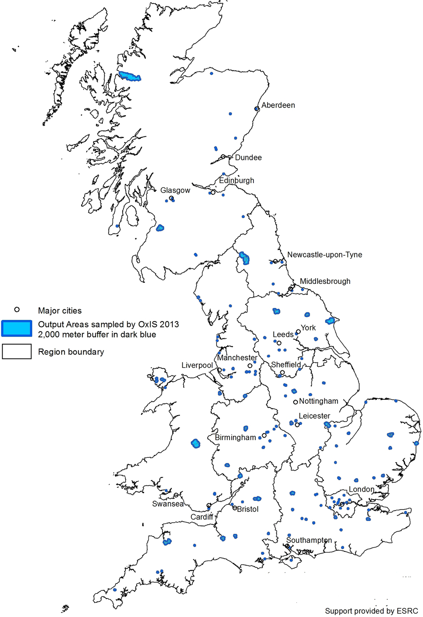
Output areas sampled by Oxford Internet Survey 2013.
OAs are the fundamental building block of the British Census. They are the smallest geographical area for which the British 2011 Census reports data. OAs are intended to have a minimum size of 40 households and 100 people and a maximum size of 250 households and 625 people and are designed to be as socially homogeneous as possible (based on household tenure, dwelling type, and urban/rural category). Scotland conducts a separate census, although the Scottish and English/Welsh censuses are coordinated, so that the questionnaires are similar, the enumeration is on the same day, and the reporting is similar. OAs in Scotland are smaller, with a minimum size of 20 households and 50 people, and homogeneity is not a criterion in their construction (Office of National Statistics [ONS], 2014). In the actual census data, the largest OA has 4,092 people and there are 108 OAs with populations greater than 1,000. The census documentation provided by the ONS does not explain why these large OAs exist. The OAs are central to this project since they exist in both the census and OxIS. We use the information on Internet use in OxIS to estimate Internet use (and other variables) for all census OAs across Britain.
We create our estimates using a technique called SAE. SAE addresses two fundamental problems. First, survey data are not available for subnational areas. No one knows, for example, the proportion of Internet users in Glasgow, Manchester, or Cardiff because national sample surveys don’t have enough respondents in those cities to make reliable statistical estimates. National surveys like OxIS are not designed to estimate small areas. The sample size of the survey is too small to make detailed inferences about the geographies of digital inequality below level of the 11 British regions, but OxIS uses a random sample of OAs and this opens up a range of possibilities.
Second, the census enumerates everyone and census data are available for very small areas. However, the census is very expensive and it collects few variables. It collects no data whatsoever on Internet use or Internet activity or mobile use of the Internet. This is a problem because detailed information on the Internet use of the population in local areas is valuable to identify areas that would benefit most from policy intervention. Thus, small area data are essential to understand where to target efforts to tackle problems like limited Internet access or limited ability to use the Internet. OxIS, on the other hand, is a very rich data set with more than 550 variables measuring all kinds of Internet activity.
By combining the richness of OxIS survey data with the comprehensive small area coverage of the census, we can use the strengths of one to offset the gaps in the other. Specifically, we follow a two-step process. First, we use the information that is reliably available in OxIS to create a model that estimates the proportion of Internet users in an OA. Second, we use the parameters from this model combined with census data to estimate the proportion of Internet users each OA in Britain. Once these estimates are available, we aggregate the estimates up to higher levels of geography. In this way, we can estimate Internet use in Glasgow, Manchester, and Cardiff as well as other small areas in Britain. This procedure is called indirect, model-based, or synthetic estimation. In recent years, such SAE techniques have been widely used throughout Europe and North America (e.g., Molina & Rao, 2010; Simpson & Tranmer, 2005; Twigg & Moon, 2002).
This procedure assumes that if the demographic characteristics of individuals influence their Internet use, then small areas will be different from each other to the extent that the demographic characteristics of their respective populations differ. 6 For example, age is a fundamental variable that influences most Internet variables. If age were the only predictor of Internet use, then small areas would only differ in Internet use if the age profile of their population differed. So a strong argument can be made for assuming that we can use differences in the area demographic profile to predict area differences in Internet use.
This process has the advantage that it allows us to directly test our research question about spatial effects versus demographic effects. There are two possibilities. First, if there are spatial effects—contextual effects—on Internet use, then they will show up as statistically significant after we introduce our demographic controls. If the apparent spatial effects are simply the result of differences in the demographic profile of different geographic areas, then the spatial variables will not be significant after we control for demography.
The methodology works because OxIS data collection was based on small geographic areas; that is, OAs. Britain is virtually alone in using this approach. Almost all other countries collect Internet data using random digit dialing telephone interviews. This includes most of the countries that are part of the World Internet Project like the United States, Canada, Sweden Australia, New Zealand, and Switzerland (Russia is an exception; Cole, 2012, 2013). It also includes the Pew Internet and American Life Project data. Eurostat assembles Internet data collected from national household surveys. But many countries collect their household data from telephone, mail, or web-based surveys (or a combination). This includes Germany, France, Austria, Sweden, Finland, the United Kingdom, and others (Eurostat, 2014). Telephone, mail, and web-based surveys cannot be used for SAE because respondents are randomly scattered across the country and do not have the necessary geographic concentration. This means that most large countries cannot use SAE to estimate Internet use in small areas.
There are many types of SAE models, see Rao (2003) for a summary. The fact that we have OxIS data on relatively few OAs limits our choice of methods. We can directly estimate the proportion of Internet users in only the OAs sampled by OxIS, so we can’t use any technique that relies on direct estimation. Other techniques that combine model-based estimates with direct estimates—such as generalized regression synthetic estimators, composite estimators, or Fay-Herriot estimators—cannot be used for the same reason; the direct estimates are available for too few OAs. Instead, we use a model-based procedure.
We estimated the parameters of our model using a linear, two-level mixed model. The first level is the 134 OA pairs; the second level is the 260 OAs. We chose this procedure because it allows for inclusion of demographic variables while taking into account the fact the respondents in each OA and each OA pair will be more alike than a random sample of the population as a whole. Taking into account the structure of the clustering of respondents in OAs improves the accuracy of confidence intervals and significance tests. These confidence intervals will generally be smaller and more conservative than confidence intervals that ignore the clustered data (Goldstein, 2003). We include five fixed effects variables—region, age, lifestage, gender, and education—and a single random effects variable, OA pairs. These are random intercept models, to account for the fact that different OA pairs will have different overall levels of Internet use.
We weighted each OA according to the number of respondents, so that OAs with more respondents (which have smaller standard errors) are weighted more heavily. Respondents themselves are counted based on poststratification weights that were created, so that the sample matched the British population on gender, age, region, rurality, ACORN code, and household size (see Dutton & Blank, 2013, for details). Since these are weighted mixed models, simple R 2s are not available and we report BIC.
Variables
The data are proportions at the OA level; in the jargon of mixed models, this is an area-level model. We cannot use individual-level covariates because the census does not provide individual-level microdata; it only makes public summary data for each OA. The dependent variable is the proportion of Internet users in each of the 260 OAs. Internet use is measured by responses to the OxIS item “Do you, yourself, personally use the Internet on whatever device at home, work, school, college or elsewhere or have you used the Internet anywhere in the past?” This broad question asks about any kind of Internet use. It encompasses Internet use out of the home, such as in a library or community center, mobile use, and in remote rural areas, possible use in another town. We measure spatial effects using Region, a collection of 10 dummy variables; Scotland is the omitted region. Gender omits males. Age is a seven-category variable. Preliminary work showed that the relation between age and Internet use is piecewise linear. The proportion of Internet users has a single shallow slope between age 14 and 51. There is a discontinuity beginning at age 52 where the slope changes abruptly; it remains linear, but it is much steeper. Since age is always a strong explanatory variable, we wanted to capture as much variation as possible. We divided age into three categories between age 14 and 51, with approximately equal number of cases in each category. Because the slope was steeper for people age 52 and above, we created four categories each containing approximately equal numbers of cases (see Table 1). The four categories balance our desire for as much fine-grained result as possible with the need for a minimum number of cases in each category. The disadvantage of this approach is that the age categories are not nice round numbers ending in zero or five. Lifestage is a four-category variable where we combined census categories to match the OxIS categories: student, employed, unemployed, and retired. For the four-category education variable, we also combined census categories to match the OxIS categories: no qualifications, secondary school, further education, and higher education. All variables are measured as proportions in all models. Table 1 shows the characteristics of our sample and of the census as a whole. Notice that the sample closely matches the census, particularly for age, gender, and region. In education, OxIS matches the percentage of people with secondary school or university qualifications, but it is different for people with no qualifications or further education. For lifestage, the percentage of students and percentage of unemployed match while the OxIS estimates fewer employed and more retired people. These differences are mostly due to the difficulty of matching census categories to OxIS categories.
Comparison of OxIS With Census Data (%).
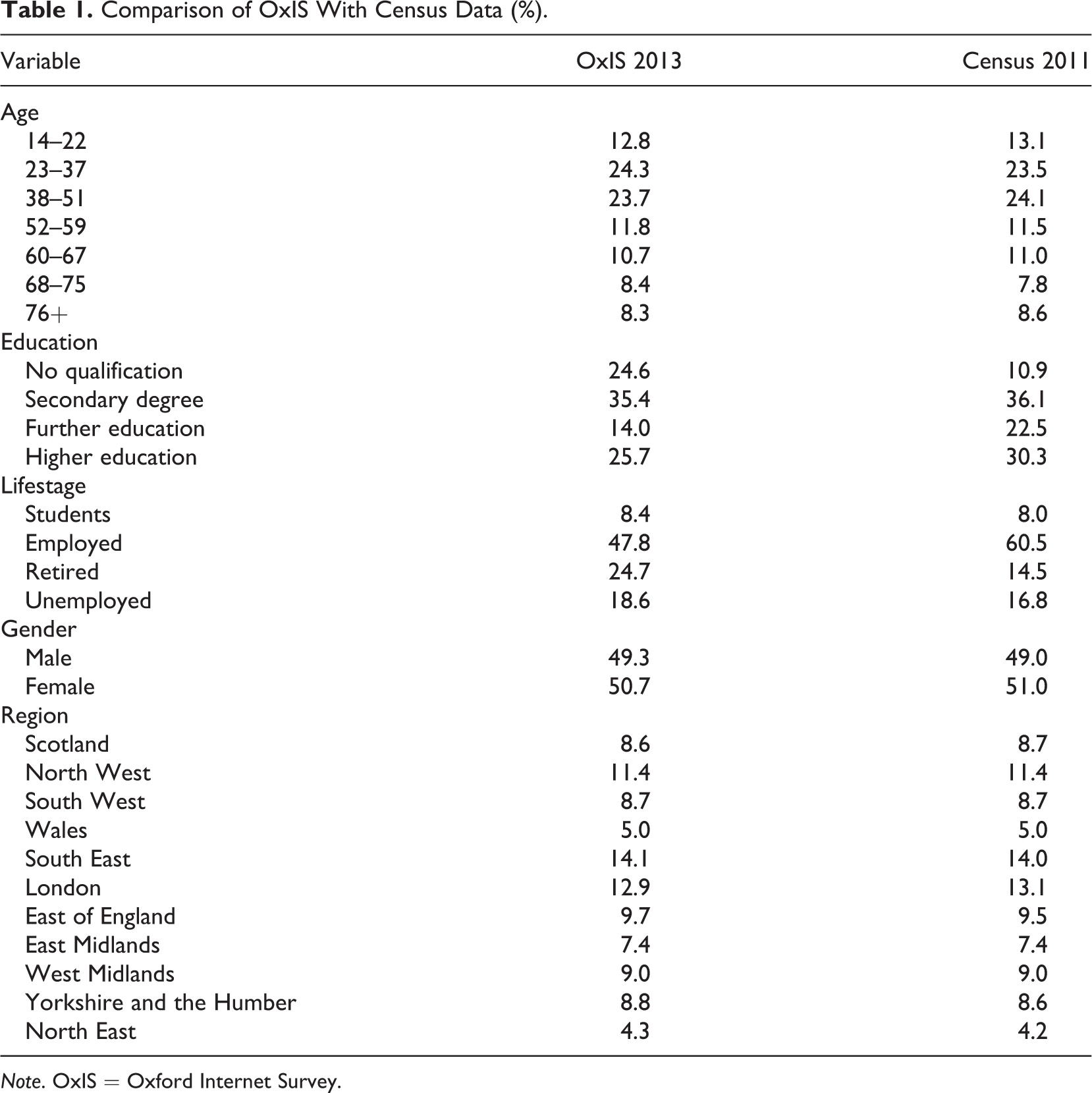
Note. OxIS = Oxford Internet Survey.
British administrative geography is a complicated structure filled with inconsistent names. Although there are additional administrative units, we will report data on two levels: regions and subregions. At the top level are 11 regions: nine English regions plus Wales and Scotland. Each region has a subregional structure with different names. Scotland is subdivided into 32 council areas. Wales is divided into 22 unitary authorities. England has a complex structure that subdivides the regions into 32 London boroughs (plus the City of London, which is not a borough), 27 counties, 56 unitary authorities, and 36 metropolitan districts. 7 To avoid this confusing nomenclature, we refer to all of the subregional divisions by a single name, “local authority districts” (LADs). OAs are much smaller than LADs and they are contained entirely within LADs. LADs vary widely in area and population; the number of OAs in a LAD ranges from 31 in the City of London to 5,486 in Glasgow, with a total of 227,759 OAs in Britain.
Results
We begin by mapping three key independent variables to give readers a sense of the geographic variation in Britain. Figure 2 shows a map of the percentage of elderly people in each LAD. Since we are interested in Internet use, we use the point where use begins its precipitous drop to define elderly as people over age 51. 8 The darker black lines are regions; LAD boundaries are in gray. The six-category scale used for shading emphasizes the extreme values. The lowest and highest categories each have 5% of LADs. The categories next to the extreme categories each contain 15% of LADs, and the middle categories each contain 30% of the LADs. Notice the strong spatial patterns, which seem to be associated with an urban–rural divide. Large cities, especially London, but also Manchester, Birmingham, Cardiff, Glasgow, Aberdeen, and others, stand out because they have relatively few elderly people. Areas like western rural Scotland, central Wales, and Cornwall have a much higher proportion of older people. In general, regional differences seem to be less strong than the urban–rural differences.
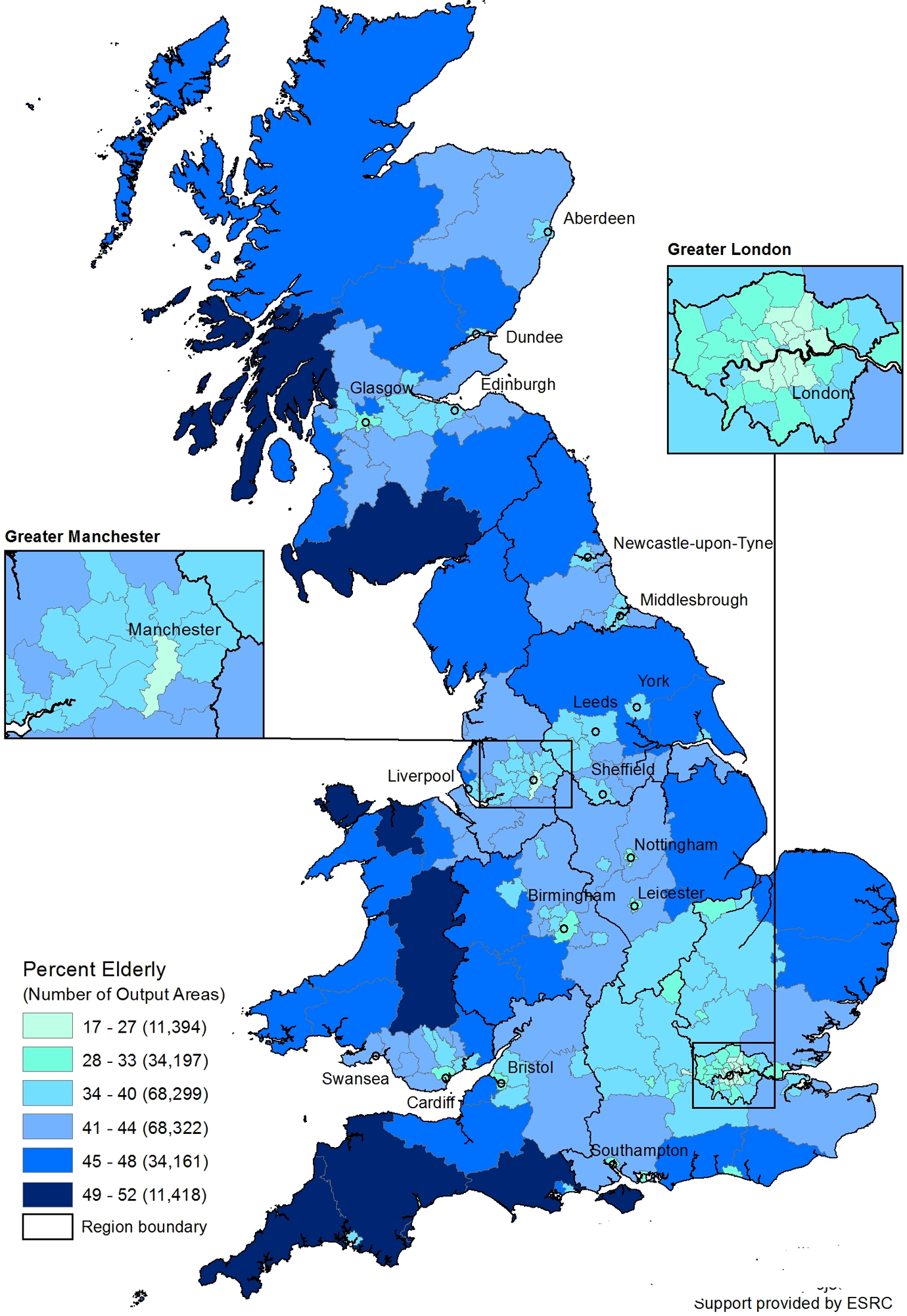
Percent elderly.
Figure 3 shows a map of the percentage of people employed in each LAD. Again there are distinct geographic differences between place, but the patterns are different from the geography of age. With some exceptions, like Birmingham, there is no apparent urban–rural difference. London, for example, has boroughs in both the highest and second lowest categories of percentage employed. The absence of an urban/rural divide may be because cities are home to large numbers of young people who are students and not employed. The lowest percentages of employed people are in western Wales, the North East of England, and southwestern Scotland. The highest percentage of employed are in the south center and northeastern Scotland.
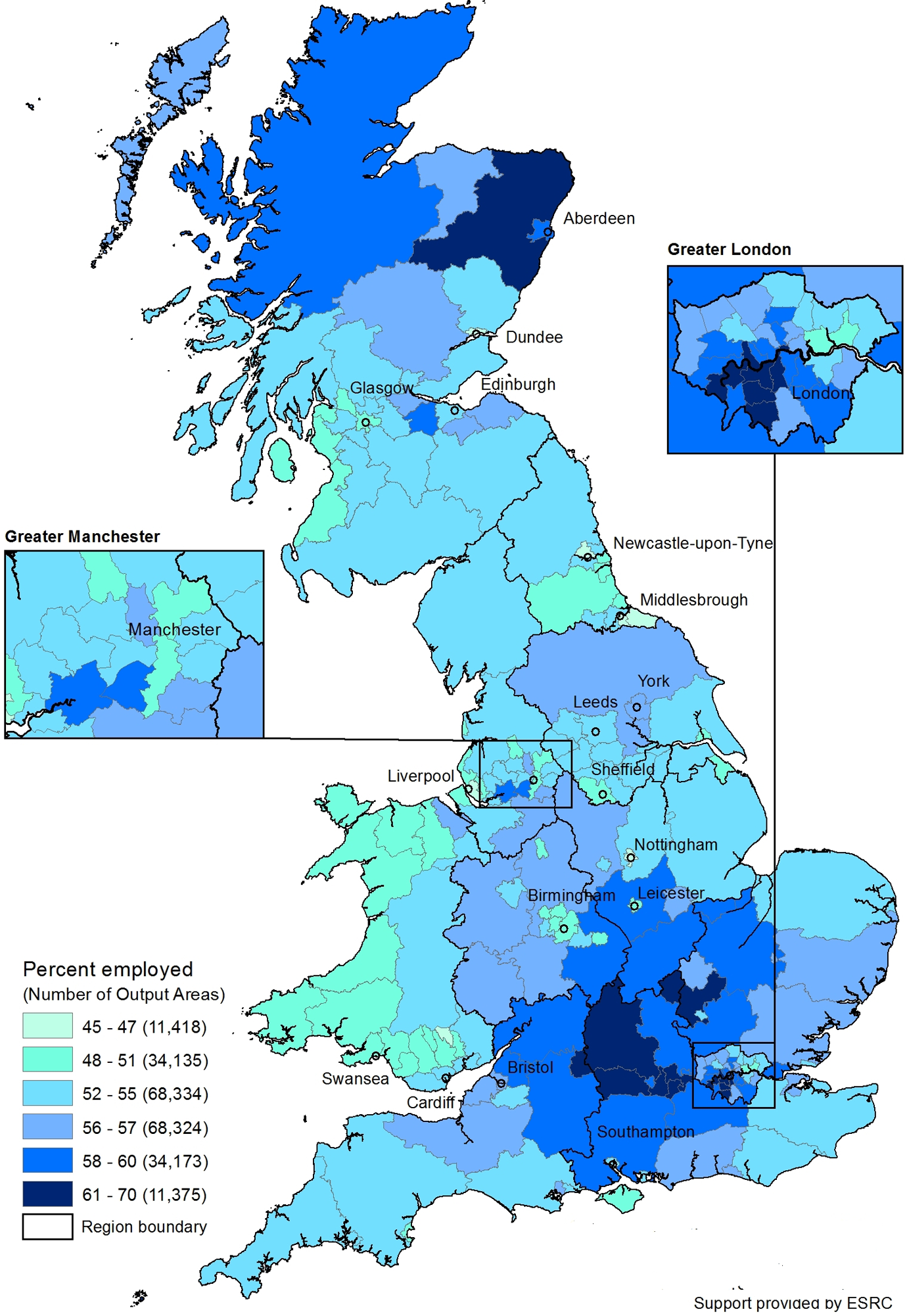
Percent employed.
The third map (Figure 4) displays the percentage of people with a higher education degree. We again see a diverse spatial pattern. London has some LADs in the highest category and some in the second lowest. Edinburgh also stands out in the highest category. Some university cities like Aberdeen, Cardiff, and York stand out from their surrounding countryside, but Leicester and Swansea, also home of a university, are in the second or third lowest category. The South East tends to have more highly educated people, while the East Midlands, southern Wales, and southwestern Scotland tend to have a smaller percentage of people with a university degree.
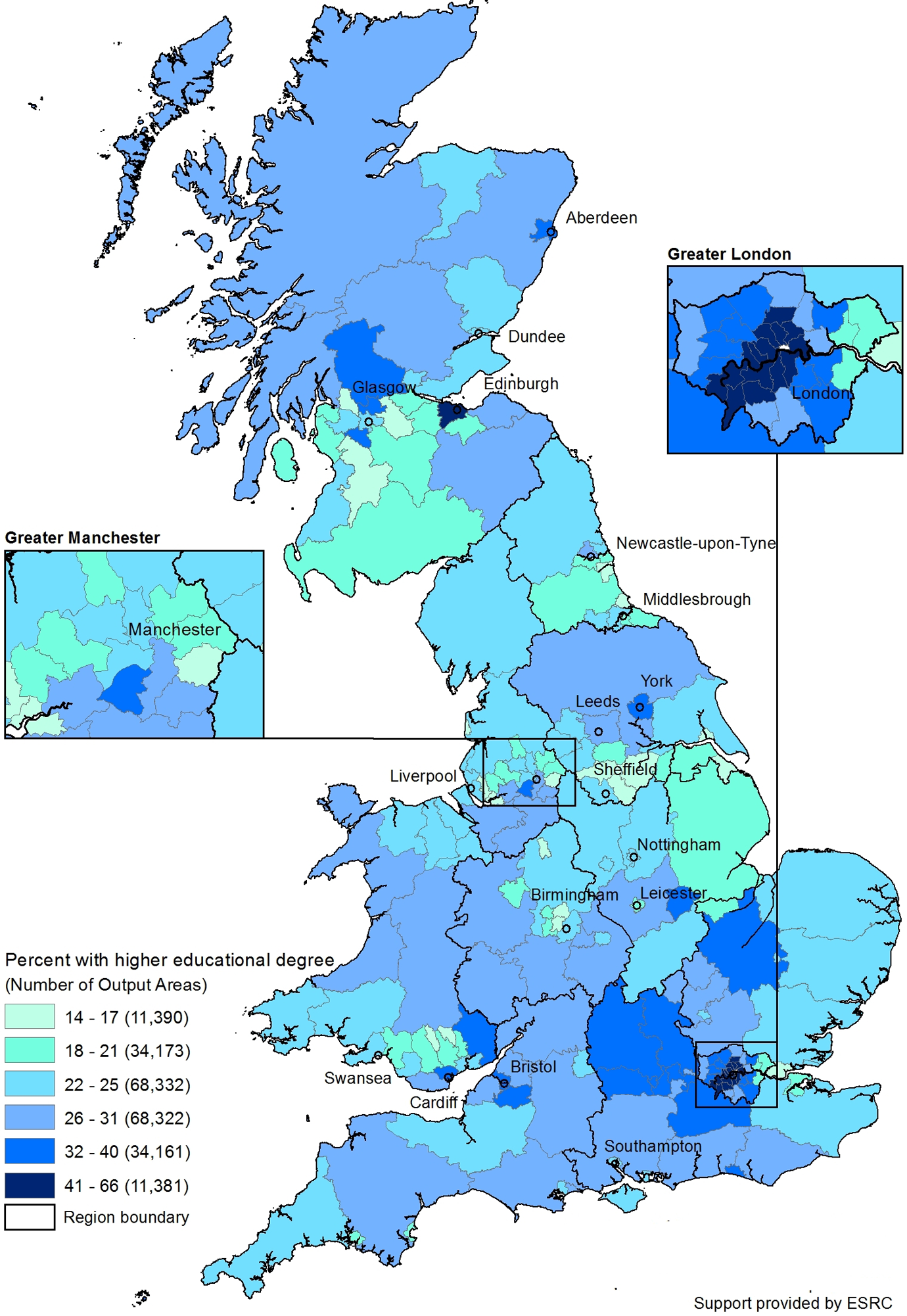
Percent with higher education degree.
The first stage of our procedure was the estimation of the coefficients from the OxIS survey (see Table 2). Table 2 shows three mixed models with different independent variables. Model 1 includes age, education, and lifestage; Model 2 adds gender; and Model 3 adds region. The data have been aggregated to the OA level; thus, N = 260 for all models.
Mixed Models Estimating the Proportion Internet Users.
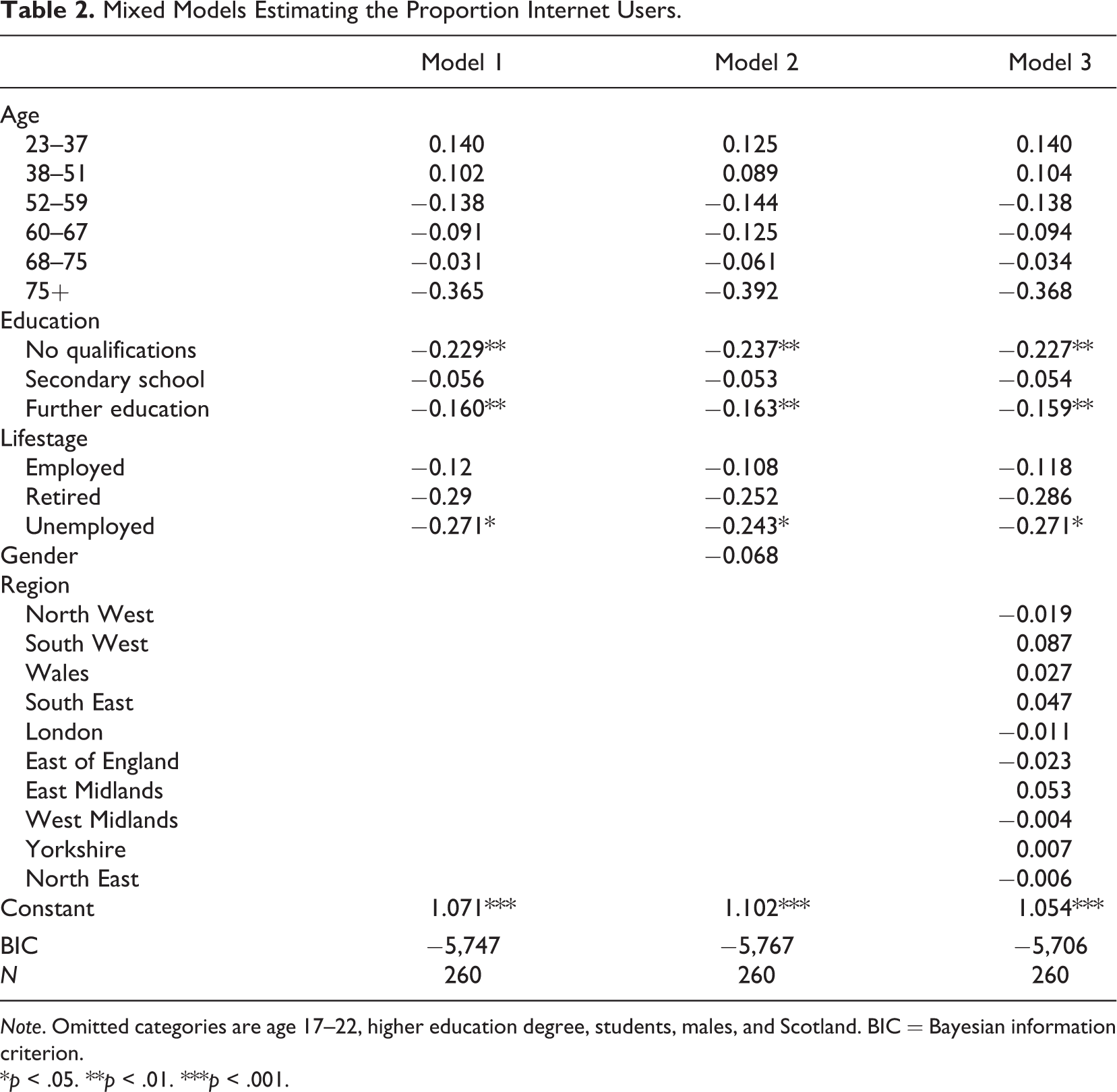
Note. Omitted categories are age 17–22, higher education degree, students, males, and Scotland. BIC = Bayesian information criterion.
*p < .05. **p < .01. ***p < .001.
The signs and sizes of coefficients are consistent with previous research on Internet use. The age coefficients turn negative and are largest in oldest age category; older users are more likely to be nonusers. Since higher education is the omitted category, all the education coefficients are negative and they are largest for least educated people; less educated people are less likely to use the Internet. The lifestage coefficients are all negative because all lifestage groups use the Internet less than omitted category, students.
Age alone accounts for about 37% of the reduction in the residual variance, so why are none of the age dummy variables significant and why did we leave age in the model? The reason is collinearity. The largest condition index for the model is 27. Auxiliary regression shows that every age dummy variable is collinear with both education and lifestage dummy variables. Collinearity also influences the education and lifestage variables, which accounts for the fact that they are not highly significant. Collinearity increases the standard errors of the coefficients, which is why they are not significant, but the coefficients are not biased by the collinearity and predictions are not damaged by collinearity. Since our goal is to build a prediction model, we have no hypotheses about the size or direction of any coefficients, and we do not interpret the coefficients, so we did not attempt to mitigate the collinearity. We left the age, lifestage, and education dummy variables in the model. Gender in Model 2 is also not statistically significant, and it increases BIC. Auxiliary regressions show that it is not collinear with anything; it is just not significantly related to Internet use. We therefore elected to not include it in any further analysis. None of the region dummy variables are statistically significant in Model 3. Again, collinearity is not the issue. The largest condition index for Model 3 is virtually identical to the largest condition index for Model 1. Auxiliary regressions showed that none of the other independent variables are significantly related to any of the region dummy variables. We elected not to include region in our predictive model. Because Model 1 includes all statistically significant variables, we used the coefficients from that model for the SAE.
The results of the SAE are in the map in Figure 5. We present the data at the LAD level. LAD use is a population-weighted average of all the OAs in the LAD. Darker shading on the map indicates higher Internet use in a LAD. We begin by discussing the areas with above average Internet use, the three darkest shades. The highest Internet use is concentrated in the southeast, and London particularly stands out. Estimated Internet use in the darkest areas is 88–89%, concentrated in London plus Reading to the west of London and Leicester. The LADs with 84–87% use stretch in a “C”-shaped band anchored in London and sweeping north. Bristol, Southampton, and Nottingham also have high levels of estimated use. The rest of the south, interestingly including Cornwall, has above average usage levels of 78–83%. Cornwall (2007) may be above average because of its above average level of broadband use. Leeds, York, and Manchester are also in this category.
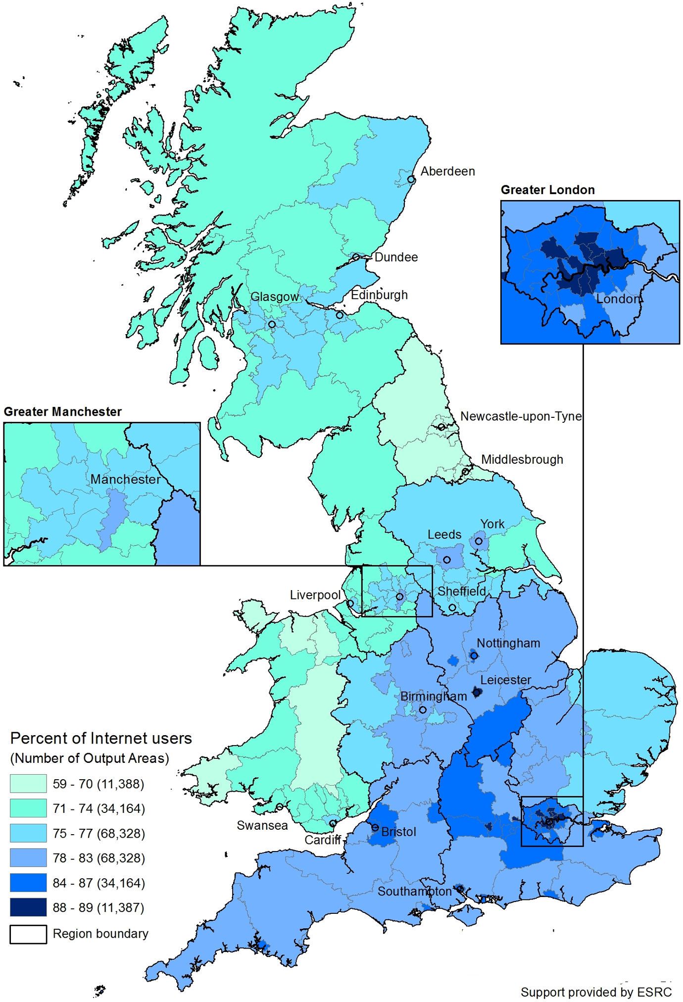
Estimated percentage of Internet users.
When we look at the below average LADs, the middle category, 75–77% Internet use, they form two blocks. One surrounds southern England, covering east of England, along the Welsh border, and in the Midlands surrounding Leeds, York, and Manchester. The other block is in Scotland, in the belt between Glasgow and Edinburgh and up to Dundee, and surrounding Aberdeen. Wales is composed of both of the two lower categories: 59–70% and 71–74%, with the exception of Cardiff. Scotland has no OAs in the lowest category. The entire North East region is in the lowest 59–70% category.
Figure 6 adds estimates for the largest cities to the OA estimates. Much of the story is identical. Cities in southern England have the highest estimated Internet use. The second highest levels are in Wales, Scotland, and the Midlands. The North Eastern cities, Newcastle and Middlesbrough, have the lowest Internet use at 64% and 61% of the population, respectively. What is notable is how cities tend to stand out with higher Internet usage than their surrounding regions: Wales, Scotland, East Midlands, Nottingham, Leicester, Bristol, and London are all examples of this. The key exceptions are Liverpool, Sheffield, and Birmingham, possibly reflecting their relatively urbanized surrounding areas.
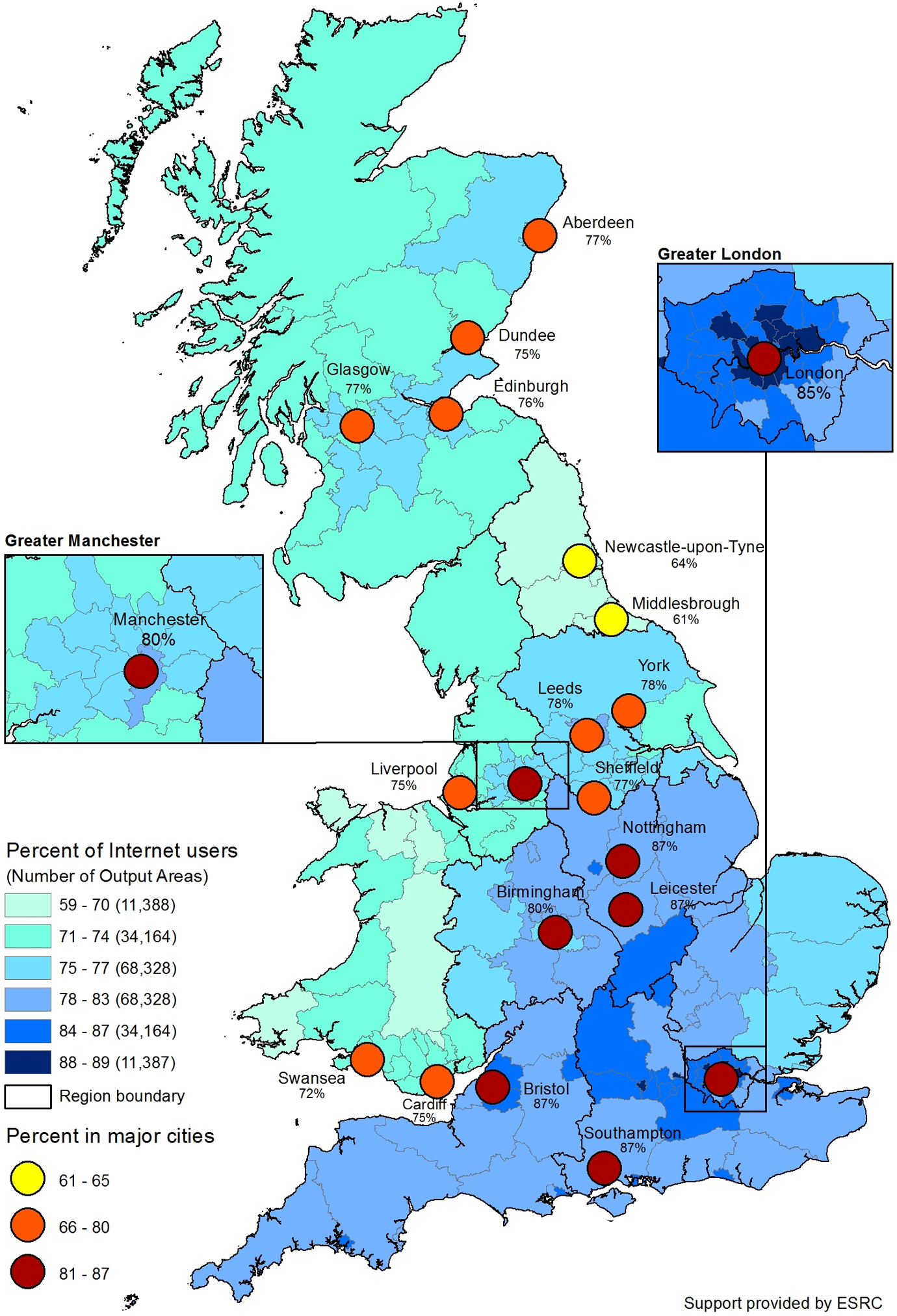
Estimated percentage of Internet users with largest cities.
Discussion
These results have offered a never-before seen look at the local geographies of Internet usage in Great Britain. However, the results do need to be interpreted with caution. There is no evidence of any issues other than ordinary sampling error in OxIS (Table 1 shows OxIS is consistent with the census), but the estimates are subject to the problems of all SAEs. Because they are estimated based on a few variables, the variance of the estimates is small. The results will have an error of exceeding the ±3% —the 95% confidence interval for OxIS—and possibly much larger. This suggests that the difference between the top two categories on the map is too small to matter, although it produces intuitively reasonable results for London.
Several other methodological issues deserve brief mention. We produced estimates at the OA level, but this report has aggregated everything to the LAD level. We do this because incorporating a large number of OAs into a single average estimate of a LAD is more likely to produce reliable values. Some of the error in the estimates from smaller OAs should wash out in the aggregated, larger LADs. We entered variables like lifestage, age, or region as a single conceptual unit. Because they are a single concept, then when one variable is part of the model, the other variables in the concept should also be part of the model. One result is that a number of variables are not statistically significant (e.g., the age variables or secondary school education), but they are conceptually important and so they remain in the model.
Beyond methodology, there are major policy implications from this work. Previously, we described the importance of the Internet to core economic, social, and political facets of contemporary Britain, but we know relatively little about who is and isn’t connected.
First, it points to several areas where there are very clearly low levels of Internet use. The North East is striking. Northeastern cities have lower Internet use than Welsh cities, and the difference is not small; it is over 10 percentage points. Furthermore, unlike other regions, Northeastern cities do not seem to be very different from the surrounding rural areas. This suggests that allocating resources to improve Internet use in the North East would be valuable. The North East needs it more than anywhere else. Although not as low as the North East, rural Wales, rural North West, and rural Scotland are the next lowest areas. They could be a secondary priority. Cornwall is actually above average, despite the fact that it has been regarded as one of the poorest areas in Britain, which was part of the reason for a major effort to extend broadband, the Superfast Cornwall funded by the European Regional Development Fund, BT and the Cornwall Council (www.superfastcornwall.org).
The most unexpected result is in Table 2. We thought that controlling for demographic variables would weaken the geographic effects but at least some geographic differences would remain. The insignificant coefficients for the region variables in Table 2 suggest that this is not the case. The regional differences that we see in the maps in Figures 5 and 6 seem to reflect the fact that demographic characteristics are unevenly distributed across Great Britain’s regions. The apparent regional differences are an epiphenomenon of demographics. This conclusion is consistent with older studies in the United States (Horigan & Murray, 2006; Mills & Whitacre, 2003).
Others (e.g., Philip et al., 2015; Salemink, Strijker, & Bosworth, 2015; Townsend et al., 2013) argue that the challenges of connecting rural communities to the Internet are due to a combination of factors, including the technological difficulties of deploying broadband away from population centers, the cost of providing digital infrastructure to sparse populations in remote areas, and the demographic characteristics of the rural population which influence levels of Internet use. The results in Table 2 suggest that the demographic factors are the most important factor. If it is true that demographics are crucial, then even if digital infrastructure were improved to be equal to urban areas, rural Internet take-up and use would still lag. This evidence directly contradicts the perspective of some studies, for example, Townsend, Sathiaseelan, Fairhurst, and Wallace (2013) or Philip, Cottrill, and Farrington (2015). It is worth repeating, as we noted in the literature review, these studies are based on a correlation and not on multivariate analysis.
The key role played by age and education raises several policy issues. First, differences in education or age are not going to disappear. To the extent that they are important, then programs based on training or technology access may do little to reduce digital inequalities. Second, although the differences in broadband access between rural and urban areas are real (Farrington et al., 2015; Townsend et al., 2013), they may make less difference than policy makers hope. Various qualitative studies (e.g., Peronard & Just, 2011) provide evidence that broadband would make a difference to many individuals, but it is not clear how these demographic realities might be overcome. Ashmore, Farrington, and Skerrat (2015, p. 274) make the reason clear when they say that “the Internet, and specifically the inclusion of superfast broadband, is heavily dependent on personal, individual contexts.” The personal contexts of rural areas include comparatively large numbers of people who are elderly and/or with less education. These demographic categories have comparatively low proportions of Internet users. Broadband access will not change this demographic fact.
Of course, this is an individual-level conclusion. It does not speak to the value of broadband for business. Broadband access may encourage business investment leading to rural economic development and jobs (Galloway & Mochrie, 2005). Furthermore, the British government’s aspirations for a digital society with services delivered “digital by default” is not possible without rural broadband. For both of these reasons, expanding rural broadband remains an important policy.
These differences in Internet use are not just a matter of a technology. The Internet has made an enormous difference in social life, culture, and our economy (Graham & Dutton, 2014). The evidence is that those who have access are able to live very different everyday lives from those who don’t: communicating with friends and family, shopping, political engagement, and job searches are just some of the types of activities for which lack of Internet access can be inherently exclusionary. Internet access provides formal and informal education opportunities, and it promises to provide better access to health care. Digital inclusion is an individual choice, but the uneven geographies of access point to exclusionary factors preventing some who would like to be connected from ever getting online. Our hope is to contribute to this effort by more closely pinpointing the areas of greatest need.
What’s Next?
We have used a straightforward measure of Internet use versus nonuse as our dependent variable. Similar techniques could predict and map a variety of other variables. For example, we could take a more nuanced view of how people use the Internet. The patterns of mobile use versus fixed-line use may differ geographically and could be mapped. We could separate work-only users, teenagers using social media, or other subsets. In particular, the 10 major Internet activities (Blank & Groselj, 2014) could be mapped. These include such things as entertainment use, information gathering, commerce, and content production. In addition, the amount of use and the variety of uses could be mapped. All these are major issues and their geographic distribution has never been tracked.
We are limited by the variables available in the British census, but we have not yet used all variables that are available. A similar technique could be used to examine possible urban–rural differences in more depth, the index of multiple deprivation, occupation, and socioeconomic status measured by National Statistics Socio-economic Classification (NS-SEC). However, in the prior work with OxIS, these variables have not been strongly predictive, which is why we did not use them in this article. Exploration of interaction effects is also desirable.
We have aggregated the OAs to LADs but this begs the question what is the appropriate spatial unit? City? Except for the largest cities, we have not explored intraurban variation. A future paper could highlight intraurban variation in Internet use. In a time of widespread commuting, where people sleep, which is what census measures, is not the only way to capture the location of Internet use. Where they work or go to school may also be relevant. One reason why a city like Leicester may be relatively low despite its university is that some of the students who attend the university may not sleep in Leicester. The increasingly dispersed settlement patterns accompanied by long commutes to work may be influencing the results. Of course, this explanation is speculative but we hope that others will build on this article to explore travel to work area and other levels of aggregation.
We have been working with census data but other geocoded data are available. The relationship between geocoded data like tweets, Wikipedia edits, social network site use, and social structural variables has never been explored. Without these sort of SAE techniques, it is impossible to describe the characteristics of users of these social media in terms of gender, age, occupation, politics, marital status, and other vars. Having the capacity to do this opens a new area for social media research. More theoretically, ask how we might expand some of the insights from OxIS using traditional (the census) and unconventional (social media data shadows of places) means. Ultimately, this work leads us to ask what methods are appropriate to measure local-scale geographies of digital participation.
Footnotes
Authors’ Note
The data have been deposited in the UK Data Archive under the name “Geography of Digital Inequality.”
Declaration of Conflicting Interests
The authors declared no potential conflicts of interest with respect to the research, authorship, and/or publication of this article.
Funding
The authors disclosed receipt of the following financial support for the research, authorship, and/or publication of this article: This work was supported by the Economic and Social Research Council (Grant ES/K00283X/1).