Sage Journals: Discover world-class research

Abstract

This manuscript details the different attributes associated with the problem of common-method variance. First, upon defining validity, we review the two primary ways by which scholars attempt to control for common-method variance, and in doing so discuss their merits. Second, we provide two alternative explanations that may also account for the appearance of disparate correlations, neither of which have to do with common-method variance. Finally, we offer a set of parsimonious solutions for the problem of common-method variance, namely CFA without correlated residuals or modeled method factors. Overall, the purpose of this manuscript is to provide guidance for organizational communication scholars when dealing with this problem.

Keywords

common-method variance specific factor error survey designs multitrait-multimethod matrix

Introduction

Over the years, organizational communication scholars have made increased use of quantitative methods (e.g., Manata & Fu, in press; Miller et al., 2011). This increase in use has yielded a spate of different quantitative approaches, the most common of which is the survey design (see Stephens et al., 2017). Preference for this method likely rests on the lack of other practical alternatives for collecting data from real organizational members. Nevertheless, it is not uncommon for cross-sectional survey designs to be approached with a healthy dose of skepticism.

One reason for such skepticism stems from the purported confounding nature of shared- or common-method variance (e.g., Podsakoff et al., 2003). Concerns about common-method variance can be traced back to the work of Campbell and Fiske (1959), who suggested that using the same method or measure could either artificially inflate or attenuate effect sizes. Despite having been challenged by others (e.g., Conway & Lance, 2010; Spector, 2006), such concerns have remained pervasive in fields where the same method (e.g., survey) is used to investigate associations between different constructs (e.g., see Baumgartner & Weijters, 2021; Kaltsonoudi et al., 2022; Malhotra et al., 2006). Organizational communication constitutes one such arena (see also Stephens et al., 2017). Indeed, a perusal of the available literature will show that common-method variance is a problem mentioned frequently by organizational communication scholars (e.g., see Child & Shumate, 2007; Fu, 2022; Manata & Fu, in press; Rice et al., 2017; Tucker et al., 2013).

Such concerns are perhaps justified, for constructs that are employed commonly in organizational communication research are likely prone to the influence of method factors. For example, when examining the constructs of organizational performance and commitment (e.g., Manata, 2023), concerns about social desirability biases, halo effects, etc. are intuitive and even unremarkable (e.g., see Podsakoff et al., 2003). Importantly, if the aforementioned constructs were confounded by some unknown method factor, then any inferences made would also be confounded. In this manuscript, we discuss the merits of various strategies that attempt to deal with this problem. Because common-method variance has not been addressed adequately in the organizational communication arena, we believe that this essay will be of decided value to those that perform quantitative organizational communication research (e.g., Child & Shumate, 2007; Fu, 2022; Manata, 2023; Rice et al., 2017; Tucker et al., 2013).

Further, this manuscript will inform the review process as the common-method variance problem is raised frequently during peer review, often creating a vexing problem for authors (see Conway & Lance, 2010). As an example of how such concerns might arise, one reviewer for the International Communication Association queried recently, “your sample had organizational members from many different organizations, how did you address common method biases?” Comments such as these are frequent and suggest a profound misunderstanding of the problem. In this manuscript, we endeavor to correct such misperceptions.

We begin by defining method and validity and defining further the problem of common-method variance. We also examine the merits of different commonly-used remedies, consider alternative explanations that might account for differences in effect sizes, and end by offering a set of parsimonious solutions to this problem. In doing so, we offer a discussion of the common-method variance problem at two different levels of analysis—item- and trait-level –mimicking the way the problem is discussed in different literatures. Overall, the aim of this manuscript is to provide an overview of the common-method variance problem for organizational communication scholars who deal with this problem frequently.

What Constitutes a Method

To measure something consists of the process of assigning numbers to the values of a variable. One way to define a method is in terms of the point of view of the person(s) producing the measure (Cushman, personal communication, 1973). Investigators might attempt to control (i.e., induce) an independent variable, in which case the value of the variable is determined by the investigator. We refer to this method as the experienced mode. It applies only to experimentally-induced independent variables. Second, self-report can be employed to measure a variable. We refer to this method as the experiencer mode. Finally, observations by someone who is neither the investigator nor the subject of study can be employed as a measure. We refer to this method as the experiencing mode, and this mode is broad. It could include participant observation, non-participant observation, projective or other tests scored by raters, public or private documents, coders’ rating of media content, and perhaps others.

A second way to define a method (not necessarily exclusive of the first) involves the measures having different item characteristic curves (ICC)¹. For example, attitude measures could all involve self-report but differ in that the indicators for one measure (X₁) employ Likert or Osgood Semantic Differential response scales (and hence linear ICC), the indicators for another (X₂) could employ Guttman indicators (and hence ogival ICC), and the indicators for a third (X₃) could use Thurstone indicators (and hence non-monotonic ICC).

What Constitutes Validity

Validity refers to the extent to which a measuring instrument measures what it purports to measure, and nothing else. Those assessing the validity of a measuring instrument might examine face validity, content validity, or the various forms of construct validity (e.g., discriminant validity; Campbell & Fiske, 1959; see also Cronbach & Meehl, 1955).

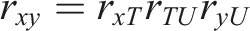
When ICCs are linear, one procedure used to assess a measure’s validity is confirmatory factor analysis (CFA). CFA assesses validity by analyzing the pattern of correlations or covariances between measures. Specifically, two theorems apply: the internal consistency and parallelism theorems (see Hunter & Gerbing, 1982).

The internal consistency theorem is defined as:

r_{x_{i} x_{j}} = r_{x_{i} T} r_{x_{j} T}

Where x_i and x_j constitute two alternative indicators of some factor, T. This theorem specifies that the correlation between two alternate indicators of the same factor equals the product of their factor loadings, i.e., the correlations between T and the x_k. Thus, this theorem tests the proposition that the correlation between any two items assessing the same factor is driven by the same unobserved latent factor and nothing else.

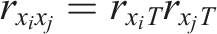
When indicators of other factors, say U, are added to the measurement model, the parallelism theorem yields predictions of the correlations or covariances between items from different factors. Specifically,

r_{x y} = r_{x T} r_{T U} r_{y U}

Where x is an indicator of the factor T and y is an indicator of the factor U. This theorem shows that the correlation between any two items from two different factors equals the triple product of both factor loadings and the correlation between the latent factors (i.e., the correlation corrected for attenuation due to error of measurement; for additional details, see Hunter & Gerbing, 1982).

In sample data, to the extent that the observed inter-item correlations or covariances are within sampling error of the predictions made by both theorems, then item responses are being driven by their respective latent factors and nothing else. An example of such a model is found in Table 1, where x1 through x4 constitute the first factor, and y1 through y4 constitute the second factor. In using the items’ factor loadings and the corrected correlation between factors T and U it can be shown that the observed correlations equal the predictions made by both theorems (i.e., the observed and implied models are equivalent). For example, the observed correlation produced between x1 and y1 is r = .20, which is exactly what is predicted by the parallelism theorem (i.e., .70*.41*.70 = .20). Similarly, the observed correlation between x1 and x3 is r = .49, which is exactly what is predicted by the internal consistency theorem (i.e., .70*.70 = .49). Applying the internal consistency and parallelism theorems to test the fit of the other observed correlations shows that the measurement model reproduces the observed data perfectly, i.e., χ² (19) = .00, Comparative Fit Index (CFI) = 1.00, Standardized Root Mean Square Residual (SRMR) = .00.²

Table 1.

Measurement Model With Perfect Fit.

	X₁	X₂	X3	X4	Y1	Y2	Y3	Y4	T	U
X1									.70	.29
X2	.49								.70	.29
X3	.49	.49							.70	.29
X4	.49	.49	.49						.70	.29
Y1	.20	.20	.20	.20					.29	.70
Y2	.20	.20	.20	.20	.49				.29	.70
Y3	.20	.20	.20	.20	.49	.49			.29	.70
Y4	.20	.20	.20	.20	.49	.49	.49		.29	.70
T	.70	.70	.70	.70	.29	.29	.29	.29	1.00	.41
U	.29	.29	.29	.29	.70	.70	.70	.70	.41	1.00

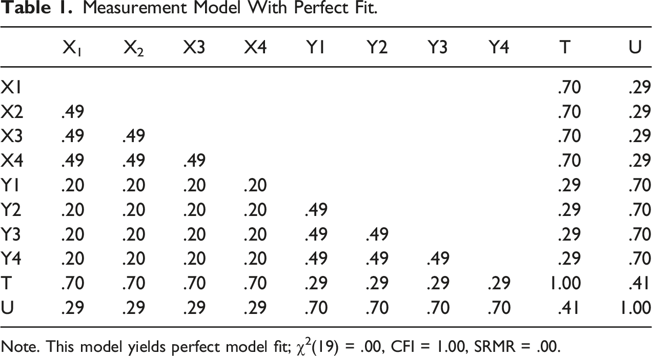
Note. This model yields perfect model fit; χ²(19) = .00, CFI = 1.00, SRMR = .00.

To the extent that observed correlations diverge significantly from the predictions made by both theorems, model fit will become attenuated. For example, if the x2-y2 and x4-y4 correlations were both changed to r = .50 (see Table 2), then the measurement model would provide a poor fit to the data, i.e., χ² (19) = 282.14, CFI = .82, SRMR = .06.^3,4 This is because there are now two large residuals of ∼.26 in the model. For example, the x2-y2 correlation (i.e., r = .50) differs significantly from the prediction made by the parallelism theorem (i.e., .70*.70*.48 ∼ .24)⁵. The same is also true of the x4-y4 correlation. Such instances are signs of model invalidity.

Table 2.

Measurement Model With Unsatisfactory Fit.

	X₁	X₂	X3	X4	Y1	Y2	Y3	Y4	T	U
X1									.70	.29
X2	.49								.70	.39
X3	.49	.49							.70	.29
X4	.49	.49	.49						.70	.39
Y1	.20	.20	.20	.20					.29	.70
Y2	.20	.50	.20	.20	.49				.39	.70
Y3	.20	.20	.20	.20	.49	.49			.29	.70
Y4	.20	.20	.20	.50	.49	.49	.49		.39	.70
T	.70	.70	.70	.70	.29	.39	.29	.39	1.00	.49
U	.29	.39	.29	.39	.70	.70	.70	.70	.49	1.00

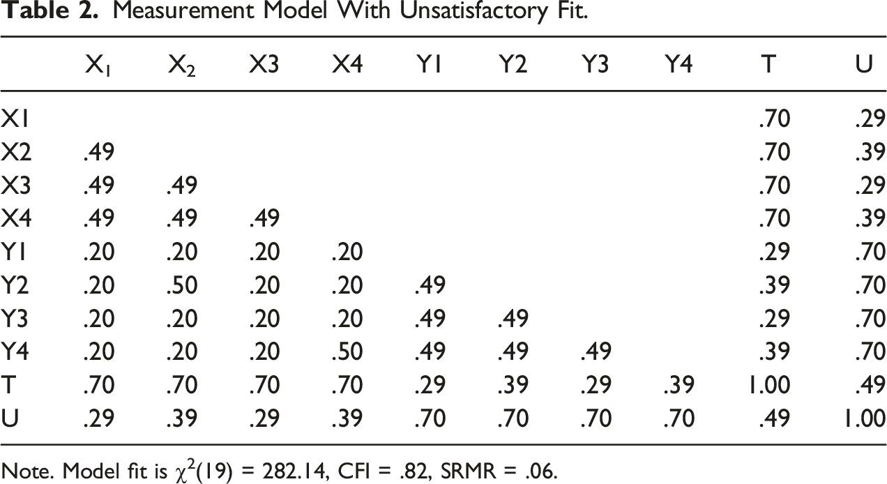
Note. Model fit is χ²(19) = 282.14, CFI = .82, SRMR = .06.

Poor model fit can occur for myriad reasons including content invalidity, non-linear ICCs, and sampling error (see Hunter, 1980), but one critical reason is the presence of unwanted specific factors common to different measures (Gerbing & Anderson, 1988). Stated differently, large residuals can occur because specific factors are shared between measures. Specific factors are factors that are systematic and unique to the measure in question (e.g., item wording) but that are also unrelated to the theoretical construct of interest (Schmidt & Hunter, 1999). For example, in addition to the construct in question, a strong need for social approval (i.e., social desirability) may also drive item responses. In this case, social desirability would constitute the specific factor.

Importantly, Podsakoff et al. (2003) specify that shared- or common-method factors constitute specific factors (p. 879). That is, when Podsakoff and colleagues refer to method factors, they equate such factors to specific factors. Podsakoff et al. also distinguish between substantive and methodological method factors. For example, in addition to the construct of interest, these authors argue that subjects’ mood may drive item responses (e.g., rating items negatively when in a bad mood), as could straight-lining responses when scale anchors are all the same (i.e., acquiescence). Nevertheless, in either case, dealing with the problem of common-method variance is equivalent to dealing with the problem of specific factor error as common-method variance constitutes a form of specific factor error.

The Problem of Specific Factor Error

As noted previously, common-method variance is problematic because it may either inflate or attenuate observed correlations in an artificial manner (Conway & Lance, 2010; Podsakoff et al., 2003). To understand how this may occur, it useful to know how specific factor variance may manifest in a measurement model. This requires a basic understanding of factor analysis.

When data are collected cross-sectionally, specific factor error is relegated to the model’s residual term (i.e., unreliability). Specifically, in a first-order measurement model, values assigned to an observed variable are driven by some unobserved latent variable and a residual (i.e., error variance). Generally,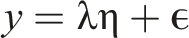

y = λ η + ϵ

Where y is the observed variable, η is the latent factor, λ is the factor loading, and ϵ is the residual or error term. In addition, ϵ can be distinguished further between random error and specific error (Lawley, 1954). That is,

ϵ = s + e

Where e is random error and s is specific error. Although random and specific error may be separated when data are collected longitudinally, these forms of error are indistinguishable when data are collected cross-sectionally (i.e., both are treated as unreliability; Boster, 2012; Gerbing & Anderson, 1984).

To the extent that unmeasured method factors are shared or common between variables, model residuals will correlate, and model fit will be attenuated significantly because the measurement model is incomplete. Indeed, if method factors are present, then a strict unidimensional model will provide a poor representation of the data because it is not accounting for all the relevant factors responsible for item responses.

If this type of invalidity is allowed to remain in a measurement model, then the correlations produced between different factors may be either attenuated or inflated artificially. As an example, consider the data presented in Table 2, which is equivalent to Table 1, save that the x2-y2 and x4-y4 correlations are now r = .50. In addition to providing a poor fit to the data, this model also yields a corrected correlation between T and U of r’ = .49 (uncorrected r = .39), which is now larger than it was when the model provided a perfect fit to the data (i.e., r’ = .41; uncorrected r = .33). Alternatively, changing the x2-y2 and x4-y4 correlations to r = −.10 would yield a corrected correlation between T and U of r’ = .33 (uncorrected r = .26), which is now noticeably smaller than r’ = .41. Indeed, to the extent that such invalidity is allowed to remain in a measurement model, effect size information will be inaccurate. Effect size information will also be substantively meaningless because the variable composites would represent more than one construct, i.e., correlations between constructs that are composites of two or more variables cannot accurately test the hypotheses they are designed to test.

One way to fix this problem is to remove the items that are plagued by such forms of invalidity. For example, the removal of x2 and y4 from the measurement model would yield a model that provides a perfect fit to the data. Moreover, the corrected correlation would once again be r’ = .41. Alternatively, removing y2 and x4 from the model would have the same effect. In either case, the result would be a measurement model in which method factors were no longer shared between measures (i.e., common-method factors would be removed). Instead, the specific factors that were once shared would be relegated to the retained items’ residual terms and treated as error variance (Gerbing & Anderson, 1988), and would thus have little to no impact on the resultant factor composite scores. Because such specific factors would be item specific (i.e., not shared with other items), and because they would be sampled independently and thus uncorrelated, they would be effectively controlled when averaged (i.e., they would cancel each other out; see Schmidt & Hunter, 1999).

Such materials may seem tangential, but we believe they are critical to understanding the common-method variance problem (i.e., where specific factors manifest, and how they may be controlled). We also believe they are critical to making a case for valid measurement, which we believe constitutes a basic prerequisite for making valid inferences. For example, if an organizational communication scholar were to investigate the effect of normative communication on performance (e.g., Manata, 2019), then valid inferences would require, at minimum, the use of valid measures. Thus, we believe establishing unidimensional measures is critical to making valid inferences. As suggested previously, this involves ensuring that available measures remain unconfounded by shared specific-factor error.

Below, a few additional procedures are discussed that have been proposed as remedies for the common-method variance problem. Importantly, such procedures are frequently employed in organizational communication (e.g., Fu, 2022; Tucker et al., 2013). Thus, we believe the following discussion is important for organizational communication scholars.

Common Statistical Remedies for Common-Method Variance

In the previous section, we suggested that dropping items from a measurement model constituted one solution to the problem of common-method variance. In this section, we consider the merits of two alternate statistical solutions used commonly as remedies: the correlated uniqueness model and modeling the common-method factor explicitly. We also discuss the merits of Harman’s single-factor test, which constitutes a popular diagnostic technique in communication science (e.g., Rice et al., 2017; Tucker et al., 2013). Each of these procedures are discussed subsequently (for a review of other proposed solutions, see Podsakoff et al., 2003).

The correlated uniqueness model involves stipulating a measurement model and then allowing error terms to correlate. As mentioned previously, common method factors, when unmeasured, are expected to manifest as specific factor errors. Moreover, because such factors are shared or common between different measures (e.g., survey items), model errors are expected to correlate; if this is left unaccounted for, it will attenuate model fit.

One proposed solution to this problem is to allow model errors to correlate. This procedure is expected to yield improved model fit because it accounts for any additional, unwanted factors that are shared between measures (Anderson & Gerbing, 1988). As an example, consider the model found in Figure 1, which uses the data found in Table 2. As mentioned previously, when a strict definition of undimensionality is used (i.e., when items load only on one factor, and residuals remain uncorrelated), this model yields a poor fit to the data: χ² (19) = 282.14, CFI = .82, SRMR = .06. However, allowing the x2-y2 and x4-y4 residuals to covary yields a model that provides a perfect fit to the data: χ² (17) = .00, CFI = 1.00, SRMR = .00. This procedure improves model fit because it accounts for the unwanted covariation left unexplained by the two-factor measurement solution. Stated differently, this procedure allows invalidity to remain in the model.

Figure 1.

Correlated uniqueness model.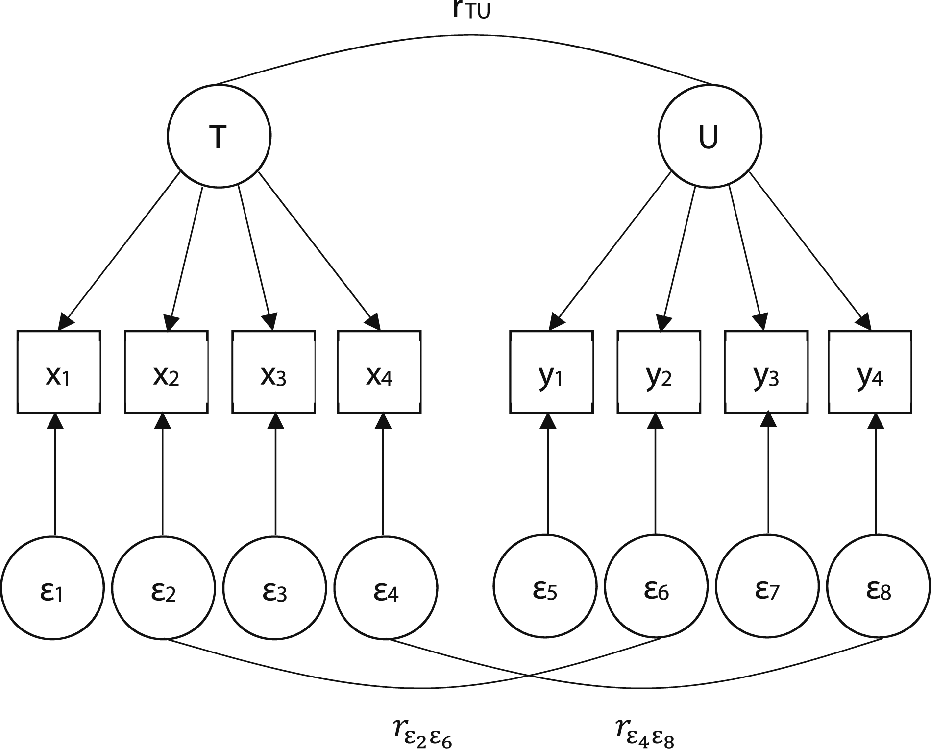

A second common way to control for common-method factors is to model the common-method factors explicitly. In this procedure, items are made to load on their respective latent factor, and also made to load on some unknown common-method factor (i.e., items are multidimensional).⁶ As an example, see Figure 2, which also models the data found in Table 2, save that two, unknown method factors are now included to account for the additional, unwanted covariation between x2-y2 and x4-y4. Similar to the correlated uniqueness model, this model yields a perfect fit to the data: χ² (12) = .00, CFI = 1.00, SRMR = .00⁷. According to Podsakoff et al. (2003), such procedures are useful because they account simultaneously for trait, method, and random error variance.

Figure 2.

Modeled method factors.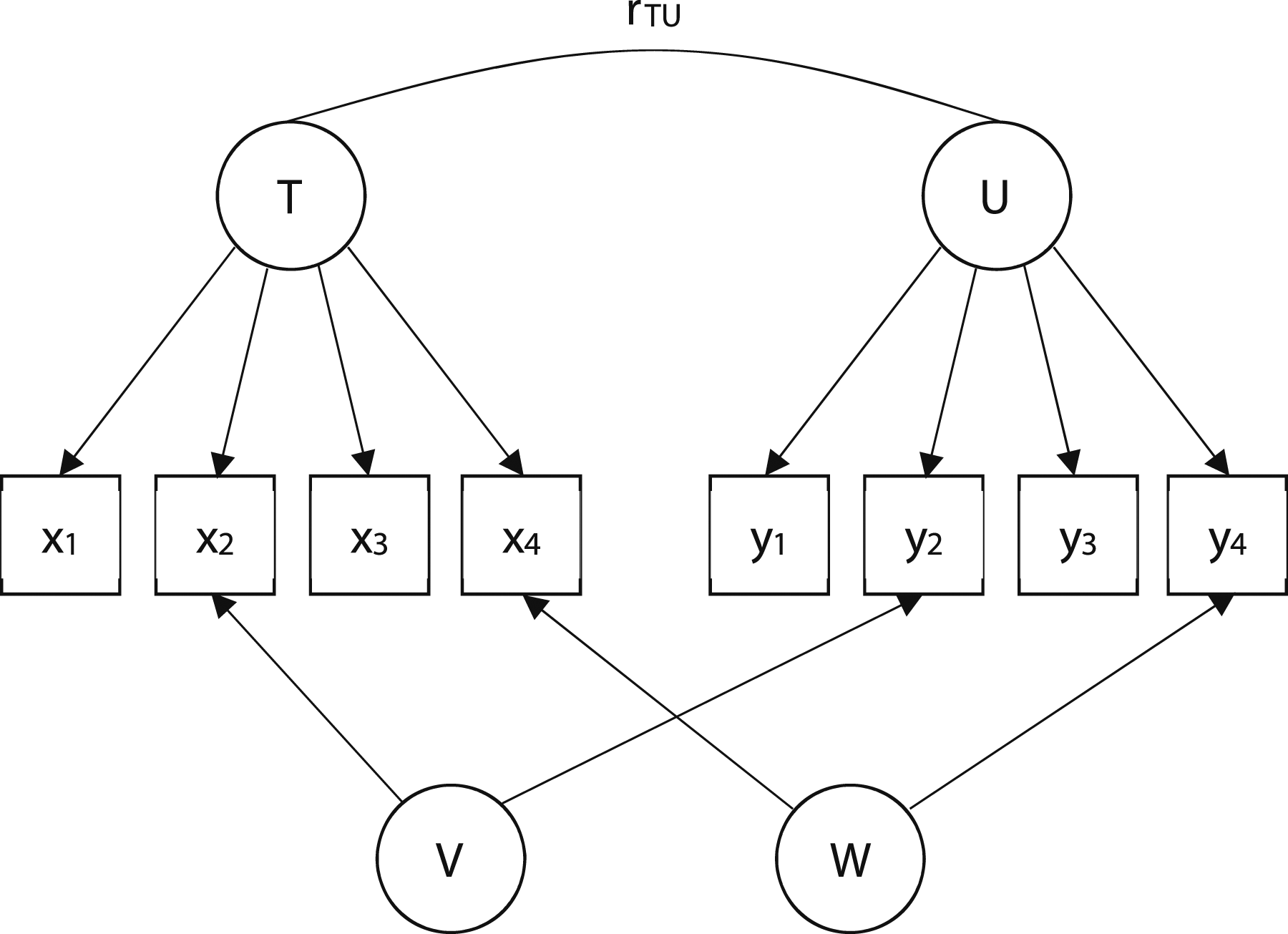

Nevertheless, there are good reasons to avoid the use of such procedures as both yield measurement models that are uninterpretable theoretically (Gerbing & Anderson, 1984). Correlating error terms constitutes an admission of additional, unknown factors driving item responses that are extraneous to the model. Similarly, modeling a confounding method factor makes it explicit that measures are in fact confounded by some unknown factor. In either case, one cannot claim that items are measuring one construct and one construct only. Importantly, when analyses (e.g., regression) are performed with confounded item composites, the interpretations of results are meaningless.

In the interest of providing a layman example, suppose that one wanted to ascertain the effect of pure sugar on health, e.g., diabetes. Now, suppose that one’s measure of pure sugar became confounded because some salt fell into the mix. In this case, with a measure of neither sugar nor salt, but a measure of sugar/salt, could one use such a measure to make valid inferences about the effect of pure sugar on diabetes? Without a measure of pure sugar, we do not believe that such an inference would be possible. This example could be extended to consider constructs more applicable to organizational scholarship. For example, presuming a scholar measured the latent factor trust (e.g., Tucker et al., 2013), one could not say that a pure measure of trust was procured if errors were correlated, or if unwanted method factors were modeled and allowed to remain in the analysis.

There are also good empirical reasons for avoiding such methods. For example, Gerbing and Anderson (1984) showed that correlating model residuals could mask the correct measurement solution. In such cases, relationships between incorrect latent factors would be estimated, and incorrect inferences would be made. Ultimately, allowing errors to be correlated in sufficient magnitude will allow false models to fit the data. Moreover, as the number of correlated errors increases, the interpretability of the model decreases significantly. Relatedly, modeling method factors has been shown to yield inaccurate effect size information. Specifically, in their large-scale simulation, Richardson et al. (2009) found that such procedures were likely to produce inaccurate corrected correlations. Consequently, these authors recommend against the general use of this method, and others have made similar points (e.g., see Conway & Lance, 2010; Lance et al., 2010; Spector, 2006). Because the use of either method increases the probability of making the incorrect inference, we believe they should be avoided.

These two procedures are noteworthy because they attempt to control for the problem of common-method variance in a statistical manner. An additional, popular diagnostic technique deserves mention, i.e., Harman’s single-factor test (see Podsakoff et al., 2003). Harman’s single-factor test is used commonly in communication science to detect, but not necessarily remedy, the problem of common-method variance. This technique attempts to detect the presence of a shared method factor by assessing the fit of a model in which all available indicators are made to load on one factor. For example, for the data found in Table 1, this technique would test the fit of a model in which all 8 indicators were made to load on one factor. If this model provided a poor fit to the data, then there would be evidence against the hypothesis that some shared method factor was explaining the available item-by-item correlations. Although such a procedure is unproblematic, we believe it is redundant with producing evidence for a valid unidimensional model. For example, as shown previously, the data found in Table 1 yields a perfect-fitting two-factor solution, i.e., χ² (19) = .00, CFI = 1.00, SRMR = .00. Unremarkably, forcing all 8 items to load on one factor yields a poor-fitting solution, i.e., χ² (20) = 391.67, CFI = .68, SRMR = .13. This is occurring because it was already shown that there are two first-order unidimensional clusters in the data, so a one-factor measurement solution will yield attenuated model fit. If a model shows that numerous first-order factors are unidimensional and valid, then forcing all indicators to load on one factor will produce a poorer-fitting model. Stated differently, if a valid model is produced without having to correlate error terms or model unwanted method factors, then the Harman’s single-factor test is not required.

Multi-Trait Multi-Method Matrices

The previous section provided a treatment of common-method variance at the item-level of analysis. One additional way scholars attempt to make inferences about common-method variance involves inspecting correlations found in a multi-trait multi-method (MTMM) matrix, i.e., a correlation matrix composed of different traits measured using the same and different methods.

An example of such a matrix is found in Table 3. In this matrix, three different traits (a, b, and c) are measured with two different methods such as self-report (X), and an objective measure (Y). According to Campbell and Fiske, numerous observations can be made from such a matrix. For example, it may be said that correlations between traits measured with the same method (e.g., X) are found in the monomethod block. Alternatively, correlations between traits measured with alternate methods (X and Y) are found in the heteromethod block. In addition, values in the diagonals in the monomethod blocks constitute reliability coefficients (e.g., coefficient alpha), whereas values in the diagonals in the heteromethod block constitute convergent validity coefficients (correlations between the same trait measured using different methods).

Table 3.

Example of MTMM.

	Xa	Xb	Xc	Ya	Yb	Yc
Xa	.81
Xb	.63	.49
Xc	.45	.35	.25
Ya	.49	.38	.27	.81
Yb	.38	.29	.21	.63	.49
Yc	.27	.21	.15	.45	.35	.25

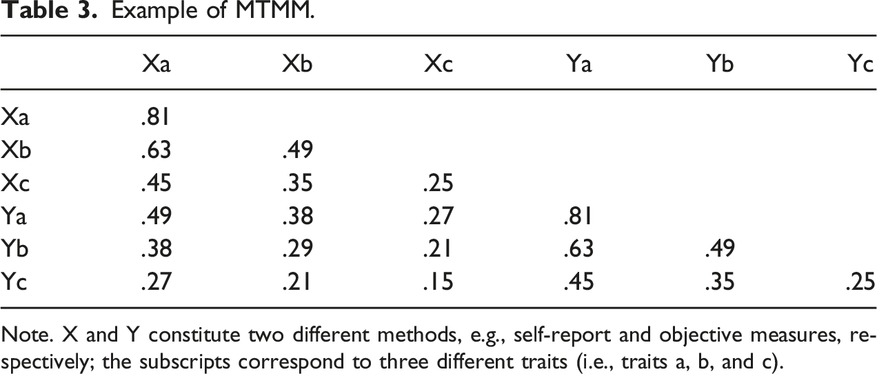
Note. X and Y constitute two different methods, e.g., self-report and objective measures, respectively; the subscripts correspond to three different traits (i.e., traits a, b, and c).

As argued by Campbell and Fiske, the problem of common-method variance can be diagnosed by inspecting and comparing the correlations found in the monomethod and heteromethod blocks. Specifically, if a correlation between different traits is stronger when measured with the same method than when measured with alternate methods, then it would be argued that the monomethod correlation was inflated due to shared-method variance.

As an example, consider again the values found in Table 3. In this table, traits a and b are correlated r = .63 when both are measured using method X (i.e., monomethod). However, the a-b correlation reduces to r = .38 when trait a is measured with method X but trait b is measured with method Y (i.e., heteromethod). Because the a-b correlation is larger in the monomethod block when compared to the heteromethod block, it would be argued that this correlation was inflated artificially by common-method variance and thus invalid.

Although this type of analysis may seem intuitive to some, there are other, more parsimonious reasons for why these correlations may differ. These explanations are provided below.

Alternate Explanations

Consider a scenario in which there are three variables, two of which were measured using self-report (experiencer mode) and the other of which was not measured using self-report (experiencing mode). Of the two self-report measures, one provides a measure of self-reported job performance, whereas the other provides a measure of self-reported job satisfaction. In addition, the objective measure yields an objective measure of job performance (e.g., sales figures). Now, consider that the correlation between the two self-report measures is r = .69, whereas the correlation between job satisfaction and objective performance is r = .49. Many would claim that this is evidence of common-method variance because the correlation produced between the two self-report measures was stronger than when the objective measure of performance was used in the analysis. Although such interpretations are common, there are at least two other viable explanations that might account for the noted difference in effect size. We term these alternative explanations differential reliability and differential validity.

One reason correlations might be discrepant when comparing mono- to heteromethods is because of differential reliability between the measures. By reliability we mean the extent to which a measuring instrument measures whatever it measures consistently. The reliability of a measuring instrument might be assessed by the test-retest method, the equivalence method, or both (Cronbach, 1951).

In general, if constructs are measured validly, unreliability attenuates correlations between constructs (Boster, 2012). One way to increase a measure’s reliability is to increase the number of parallel items or measures used in a test. For example, if a 2-item scale has a reliability of α = .60, then adding 2 parallel items to the measure will increase the instrument’s reliability to α = .75. Adding more parallel items to this measure would increase reliability further (Brown, 1910; Spearman, 1910)⁸.

We note that most objective measures of alternate constructs are 1-item measures. Moreover, although the composite reliability of a 1-item measure cannot be estimated, Schmidt and Hunter (2015) suggest that such reliabilities are likely very low (i.e., α ∼ .25)⁹. To the extent that alternate measures of the same construct evidence differential reliability, inferences made regarding the existence of common-method variance are confounded with unreliability. That is, using a MTMM matrix to make accurate inferences about common-method variance requires the condition that the available measures evidence equivalent reliability (Campbell & Fiske, 1959).

As an example, consider the scenario described previously, where the correlation between the two self-report measures of job satisfaction and performance was r = .69 and the correlation between job satisfaction and objective performance was r = .49. Now consider that the reliability of the job satisfaction measure is α = .89, that the reliability of the self-report performance measure is α = .71, and that the reliability of the objective performance measure is α = .45.¹⁰ Notably, using the correction for attenuation (see Boster, 2012) shows that these correlations are not as discrepant as the uncorrected correlations would suggest. Specifically, the corrected correlation between the two self-report measures is r’ = .79, whereas the corrected correlation between the self-report job satisfaction measure and objective performance measure is r’ = .77. Put differently, correcting these correlations for unreliability shows that they are essentially equivalent and that any differences were due to unreliability.

As a second, alternative explanation, consider that effect sizes produced using heteromethods may be discrepant because they measure different traits. That is, making inferences about common-method variance requires the condition that different methods yield alternate measures of the same construct. For instance, in our previous example, it was assumed that the self-report measure of performance was an alternate indicator of the objective performance measure. However, if this condition is not met, then comparing one measure to the other for the purposes of making inferences about common-method variance constitutes a meaningless exercise.

One way to test the extent to which two different composite measures are alternate indicators of the same construct is to perform a second-order factor analysis¹¹. The validity of second-order factors can be analyzed using the internal consistency and parallelism theorems, albeit at a higher-level of abstraction (i.e., at the trait-level of analysis; see Hunter & Gerbing, 1982).

As a demonstration of this procedure, a second-order CFA was performed on the first matrix of real data presented by Campbell and Fiske (1959, p. 86). In this matrix, there are four traits (courtesy, honesty, poise, school drive) measured using two different methods (peer ratings and association tests). As such, four different second-order factors are possible (e.g., two measures of courtesy, two measures of honesty, and so on). Notably, an application of the internal consistency and parallelism theorems to these data yields a model that provides a poor fit to the data, χ² (14) = 120.66, CFI = .89, SRMR = .11. Stated differently, although it was assumed by Campbell and Fiske (1959) that these data contained different measures of the same construct (e.g., two different measures of courtesy), this analysis shows that this assumption was false.

If this same analysis is applied to those matrices in Campbell and Fiske that include unique, analyzable information, then 7/9 (∼78%) of the matrices fail this validity requirement. Although these authors assumed that their analyzed matrices included alternate measures of the same constructs, the evidence was consistent with this hypothesis only ∼22% of the time.

In sum, when numerous methods are used to measure the same trait, there are numerous explanations for why different correlations may be produced between methods. Additionally, if either of the two alternative explanations are viable, investigators may be making incorrect inferences regarding the problem of common-method variance. For example, it may be concluded that results are confounded by an unknown method factor when the problem is instead differential reliability. Similarly, it may be concluded that the same construct behaves differently when using different methods when the problem is instead that different constructs were measured. Ultimately, when different traits are measured with different measures, we believe it is worth granting both alternative explanations additional consideration. In our experience, these alternative explanations, despite seeming self-evident, are usually ignored.

Proposed Solutions

So far, we have described the myriad ways by which scholars account for and make inferences about shared-method factors. Here, we propose a simple solution for the problem of common-method variance.

As suggested previously, one viable solution is CFA where invalid items are dropped from the analysis (e.g., removing either x2 and y4 or y2 and x4 from the models in either Figure 1 or Figure 2). We reiterate that items that conform to the internal consistency and parallelism theorems are being driven by some unobserved factor and nothing else, i.e., there are no other shared factors between items or measures. Moreover, and importantly, any remaining specific factors not common to different measures or items are controlled for by averaging the remaining items in each factor cluster. That is, because the remaining specific factors are item specific (i.e., not shared with other items), and because they are sampled independently and thus uncorrelated, they tend to cancel each other out when averaged (Schmidt & Hunter, 1999)¹². If a measurement model provides an adequate fit to the data without having to correlate error terms or model unknown latent method factors, then common-method factors are likely to be of little consequence in the analysis. Indeed, dropping items that are invalid renders a model in which items are driven by one factor only, thus eliminating the shared-method variance problem. Implementing this solution precludes the estimation of additional models that are confounded theoretically (e.g., a model in which item responses are driven by two different latent factors), and it also means that performing Harman’s single-factor test, a common diagnostic procedure, is no longer required.

This solution deals with the problem of common-method variance at the item-level of analysis, which differs from Campbell and Fiske’s (1959) treatment of common-method variance at the trait-level of analysis. Ultimately, this is a question of whether common-method factors impact item responses directly, or whether they manifest as higher-order latent factors that impact items indirectly (i.e., through the first-order factors; see Podsakoff et al., 2003). In the event of the latter occurring, CFA may also be used to rule out the possibility that some shared-method factor is present in the data. That is, the presence of a higher-order common-method factor may be inferred by assessing whether all of one’s constructs measured with one measure load on one second-order factor. If such a model were to provide an adequate representation of the data despite the apparent unrelatedness of the traits in question, then a common-method factor (e.g., acquiescence) may provide a reasonable explanation for such a phenomenon. However, in our experience, if first-order factors are unidimensional and valid, then such occurrences are decidedly improbable. Instead, it is much more likely that first-order constructs cluster for theoretical reasons, i.e., it is much more likely that second-order factors of substantive meaning are evident in the data (e.g., Cruz & Manata, 2020; Gerbing & Anderson, 1984; Hunter & Gerbing, 1982; Manata et al., 2018; Manata & Grubb, 2022; Manata & Spottswood, 2022). When this occurs, first-order factors are more likely to cluster by content, as opposed to forming one general second-order factor composed of all the available measures in the study.

Conclusion

This manuscript has detailed the different attributes surrounding the problem of common-method variance. This manuscript has also reviewed the primary ways scholars have attempted to control for common method variance; in doing so, a set of parsimonious solutions were offered (e.g., CFA without correlated model residuals). Finally, two alternative explanations were offered for instances that may be construed falsely as the confounding influence of a shared method factor when examining a MTMM matrix. This essay, then, informs organizational communication scholars about the different attributes associated with common-method variance, and hopefully assists in both the conduct of scientific research and in responses to reviewer criticism.

Footnotes

Declaration of Conflicting Interests

The author(s) declared no potential conflicts of interest with respect to the research, authorship, and/or publication of this article.

Funding

The author(s) received no financial support for the research, authorship, and/or publication of this article.

ORCID iD

Brian Manata

Notes

Author Biographies

Brian Manata (PhD, Michigan State University, 2015) is an Assistant Professor in the Department of Communication Arts and Sciences at Pennsylvania State University, University Park, USA. His research program focuses primarily on the study of workgroup dynamics and leadership behaviors.

Franklin J. Boster (PhD, Michigan State University, 1978) is a Professor Emeritus in the Department of Communication at Michigan State University, East Lansing, USA. His research program focuses on the study of social influence and group dynamics and their intersection.

References

Anderson

J. C.

Gerbing

D. W.

(1988). Structural equation modeling in practice: A review and recommended two-step approach. Psychological Bulletin, 103(3), 411–423. https://doi.org/10.1037/0033-2909.103.3.411

Baumgartner

Weijters

(2021). Dealing with common method variance in international marketing research. Journal of International Marketing, 29(3), 7–22. https://doi.org/10.1177/1069031X21995871

Boster

F. J.

(2012). Error of measurement in longitudinal designs: Defining, identifying, and correcting for specific error and transient error. Communication Research Reports, 29(3), 250–256. https://doi.org/10.1080/08824096.2012.684809

Brown

(1910). Some experimental results in the correlation of mental abilities. British Journal of Psychology, 3(3), 296–322. https://doi.org/10.1111/j.2044-8295.1910.tb00207.x

Campbell

D. T.

Fiske

D. W.

(1959). Convergent and discriminant validation by the multitrait-multimethod matrix. Psychological Bulletin, 56(2), 81–105. https://doi.org/10.1037/h0046016

Child

J. T.

Shumate

(2007). The impact of communal knowledge repositories and people-based knowledge management on perceptions of team effectiveness. Management Communication Quarterly, 21(1), 29–54. https://doi.org/10.1177/0893318907301987

Conway

J. M.

Lance

C. E.

(2010). What reviewers should expect from authors regarding common method bias in organizational research. Journal of Business and Psychology, 25(3), 325–334. https://doi.org/10.1007/s10869-010-9181-6

Cronbach

L. J.

(1951). Coefficient alpha and the internal structure of tests. Psychometrica, 16(3), 297–334. https://doi.org/10.1007/BF02310555

Cronbach

L. J.

Meehl

P. E.

(1955). Construct validity in psychological tests. Psychological Bulletin, 52(4), 281–302. https://doi.org/10.1037/h0040957

10.

Cruz

Manata

(2020). Measurement of environmental concern: A review and analysis. Frontiers in Psychology, 11(363), 1–14. https://doi.org/10.3389/fpsyg.2020.00363

11.

Cushman

D. P.

(1973). The three modes of operationism. Personal Communication.

12.

J. S.

(2022). Understanding the internal and external communicative drivers of organizational innovativeness. Communication Research, 49(5), 675–702. https://doi.org/10.1177/0093650220981299

13.

Gerbing

D. W.

Anderson

J. C.

(1984). On the meaning of within-factor correlated measurement errors. Journal of Consumer Research, 11(1), 572–580. https://doi.org/10.1086/208993

14.

Gerbing

D. W.

Anderson

J. C.

(1987). Improper solutions in the analysis of covariance structures: Their interpretability and a comparison of alternate respecifications. Psychometrika, 52(1), 99–111. https://doi.org/10.1007/bf02293958

15.

Gerbing

D. W.

Anderson

J. C.

(1988). An updated paradigm for scale development incorporating unidimensionality and its assessment. Journal of Marketing Research, 25(2), 186–192. https://doi.org/10.1177/002224378802500207

16.

Hair

J. F.

Black

W. C.

Babin

B. J.

Anderson

R. E.

(2019). Multivariate data analysis, Cengage.

17.

L. T.

Bentler

P. M.

(1999). Cutoff criteria for fit indexes in covariance structure analysis: Conventional criteria versus new alternatives. Structural equation modeling: A Multidisciplinary Journal, 6(1), 1–55. https://doi.org/10.1080/10705519909540118

18.

Hunter

J. E.

(1980) Factor analysis. In Monge

(Ed.), Multivariate techniques in human communication research. Academic Press.

19.

Hunter

J. E.

Gerbing

D. W.

(1982). Unidimensional measurement, second order factor analysis, and causal models. Research in Organizational Behavior, (vol. 4, pp. 267–320). Elsevier.

20.

Kaltsonoudi

Tsigilis

Karteroliotis

(2022). Critical review of the literature and current tendencies of the common method variance in sport management research. Measurement in Physical Education and Exercise Science, 26(2), 103–115. https://doi.org/10.1080/1091367X.2021.1949322

21.

Lance

C. E.

Dawson

Birkelbach

Hoffman

B. J.

(2010). Method effects, measurement error, and substantive conclusions. Organizational Research Methods, 13(3), 435–455. https://doi.org/10.1177/1094428109352528

22.

Lawley

D. N.

(1954). XIII.—A statistical examination of the centroid method. Proceedings of the Royal Society of Edinburgh Section A: Mathematics, 64(2), 175–189. https://doi.org/10.1017/S0080454100007433

23.

Malhotra

N. K.

Kim

S. S.

Patil

(2006). Common method variance in IS research: A comparison of alternative approaches and a reanalysis of past research. Management Science, 52(12), 1865–1883. https://doi.org/10.1287/mnsc.1060.0597

24.

Manata

(2019). The structural effects of team density and normative standards on team member performance. Human Communication Research, 45(3), 309–333. https://doi.org/10.1093/hcr/hqz003

25.

Manata

(2023). Relational balance in the workplace: Exploring the moderating role of organizational commitment. Management Communication Quarterly, 37(3), 572–598. https://doi.org/10.1177/08933189221137579

26.

Manata

J. S.

(in press). Quantitative methods in organizational communication. In Miller

V. D.

Poole

M. S.

(Eds.), Handbook of organizational communication theory and research. DeGruyter.

27.

Manata

Grubb

(2022). Conceptualizing leader–member exchange as a second-order construct. Frontiers in Psychology, 13(953860), 1–13. https://doi.org/10.3389/fpsyg.2022.953860

28.

Manata

Miller

Mollaoglu

Garcia

A. J.

(2018). Measuring key communication behaviors in integrated project delivery teams. Journal of Management in Engineering, 34(4), 1–7. https://doi.org/10.1061/(ASCE)ME.1943-5479.0000622

29.

Manata

Spottswood

(2022). Extending Rice et al. (2017): The measurement of social media affordances. Behaviour and Information Technology, 41(6), 1323–1336. https://doi.org/10.1080/0144929X.2021.1875264

30.

Martin

Guillaume

Thomas

Lee

Epitropaki

(2016). Leader–member exchange (LMX) and performance: A meta-analytic review. Personnel Psychology, 69(1), 67–121. https://doi.org/10.1111/peps.12100

31.

Miller

V. D.

Poole

M. S.

Seibold

D. R.

Myers

K. K.

Park

H. S.

Monge

Fulk

Frank

L. B.

Margolin

D. B.

Schultz

C. M.

Cuihua Shen Weber

Lee

Shumate

(2011). Advancing research in organizational communication through quantitative methodology. Management Communication Quarterly, 25(1), 4–58. https://doi.org/10.1177/0893318910390193

32.

Podsakoff

P. M.

MacKenzie

S. B.

Lee

J. Y.

Podsakoff

N. P.

(2003). Common method biases in behavioral research: A critical review of the literature and recommended remedies. Journal of Applied Psychology, 88(5), 879–903. https://doi.org/10.1037/0021-9010.88.5.879

33.

R Core Team . (2016). R: A language and environment for statistical computing. R Foundation for Statistical Computing. https://www.r-project.org/

34.

Rice

R. E.

Evans

S. K.

Pearce

K. E.

Sivunen

Vitak

Treem

J. W.

(2017). Organizational media affordances: Operationalization and associations with media use. Journal of Communication, 67(1), 106–130. https://doi.org/10.1111/jcom.12273

35.

Richardson

H. A.

Simmering

M. J.

Sturman

M. C.

(2009). A tale of three perspectives: Examining post hoc statistical techniques for detection and correction of common method variance. Organizational Research Methods, 12(4), 762–800. https://doi.org/10.1177/1094428109332834

36.

Rosseel

(2012). lavaan: An R package for structural equation modeling. Journal of Statistical Software, 48(2), 1–36. https://doi.org/10.18637/jss.v048.i02

37.

Schmidt

F. L.

Hunter

J. E.

(1999). Theory testing and measurement error. Intelligence, 27(3), 183–198. https://doi.org/10.1016/S0160-2896(99)00024-0

38.

Schmidt

F. L.

Hunter

J. E.

(2015). Methods of meta-analysis: Correcting error and bias in research findings. Sage. https://doi.org/10.4135/9781483398105

39.

Shrout

P. E.

Fleiss

J. L.

(1979). Intraclass correlations: Uses in assessing rater reliability. Psychological Bulletin, 86(2), 420–428. https://doi.org/10.1037/0033-2909.86.2.420

40.

Spearman

(1910). Correlation calculated from faulty data. British Journal of Psychology, 3(3), 271–295. https://doi.org/10.1111/j.2044-8295.1910.tb00206.x

41.

Spector

P. E.

(2006). Method variance in organizational research: Truth or urban legend? Organizational Research Methods, 9(2), 221–232. https://doi.org/10.1177/1094428105284955

42.

Stephens

K. K.

(2017). Organizational communication methods published in MCQ 2001-2015: Trends and pedagogical implications. Management Communication Quarterly, 31(1), 130–138. https://doi.org/10.1177/0893318916675735

43.

Tucker

D. A.

Yeow

Viki

G. T.

(2013). Communicating during organizational change using social accounts: The importance of ideological accounts. Management Communication Quarterly, 27(2), 184–209. https://doi.org/10.1177/0893318912469771

	Xa	Xb	Xc	Ya	Yb	Yc
Xa	.81
Xb	.63	.49
Xc	.45	.35	.25
Ya	.49	.38	.27	.81
Yb	.38	.29	.21	.63	.49
Yc	.27	.21	.15	.45	.35	.25

	Xa	Xb	Xc	Ya	Yb	Yc
Xa	.81
Xb	.63	.49
Xc	.45	.35	.25
Ya	.49	.38	.27	.81
Yb	.38	.29	.21	.63	.49
Yc	.27	.21	.15	.45	.35	.25

Reconsidering the Problem of Common-Method Variance in Organizational Communication Research

Abstract

Keywords

Introduction

What Constitutes a Method

What Constitutes Validity

The Problem of Specific Factor Error

Common Statistical Remedies for Common-Method Variance

Multi-Trait Multi-Method Matrices

Alternate Explanations

Proposed Solutions

Conclusion

Footnotes

Declaration of Conflicting Interests

Funding

ORCID iD

Notes

Author Biographies

References

	Xa	Xb	Xc	Ya	Yb	Yc
Xa	.81
Xb	.63	.49
Xc	.45	.35	.25
Ya	.49	.38	.27	.81
Yb	.38	.29	.21	.63	.49
Yc	.27	.21	.15	.45	.35	.25