Microstructure generation of long fiber reinforced hybrid composites using the fused sequential addition and migration method

Abstract

We present a fused sequential addition and migration (fSAM) algorithm to generate synthetic microstructures for long fiber reinforced hybrid composites. To incorporate the bending of long fibers, we model the fibers as polygonal chains and use an optimization framework to search for a non-overlapping fiber configuration with the desired properties. As microstructures of hybrid composites consist of materials with varying characteristics, e.g., different fiber orientation distributions or fiber volume fractions, the unit cell needs to be divided in subcells. Then, the objective function is required to account for the characteristics of the subcells individually. To ensure that the location of a fiber is restricted to its respective subcell, we apply box constraints during the optimization procedure. Depending on the materials and the manufacturing processes, the interfaces within hybrid composites show either strict separation or interlocking of the different materials. Hence, we enable selecting the box-constraint type to model the interface according to the desired composite. We provide a detailed discussion of the extensions of the original fSAM algorithm to generate hybrid composites, considering two alternative procedures to handle the box constraints during the optimization procedure. As the selection of the box-constraint type influences the synthetic microstructures, we investigate the shape of the interfacial areas and the computed effective stiffnesses. Last but not least, to validate the capability of the fSAM algorithm to generate representative microstructures, we compare the resulting mechanical behavior with experimental data.

Introduction

State of the art

Driven by the need for materials which feature high specific stiffnesses and permit to be mass-produced, fiber-reinforced composites play an essential role for lightweight technologies.^1–3 Of central importance are fiber-reinforced hybrid composites, which consist of different fiber-reinforced material systems, as they enable tailoring the material to specific requirements. In the field of hybrid composites, the continuous-discontinuous fiber-reinforced polymers (CoDicoFRP) represent an innovative material class which combines the high load-bearing capacity of the continuous (Co) reinforcement with the design freedom of the discontinuous (Dico) reinforcement. ⁴ To use CoDicoFRP for lightweight applications, tools to predict the mechanical properties are necessary which account for the heterogeneity, randomness and anisotropy of the material system. Characterizing the effective properties by experiments requires a significant expense in time and resources, especially to cover the various fiber orientation states and fiber volume fractions. As an efficient alternative, computational multiscale methods^5–7 based on the theory of homogenization^8,9 may be used. However, such methods require a geometrical description of the underlying microstructure to be given, for a start.

For fiber-reinforced composites, microstructural images may be obtained from micro-CT scanning.^10–13 However, using these real digital images as a starting point for computational multiscale methods suffers from several disadvantages. First, the expense to obtain a single image is rather high. Secondly, each image represents a specific combination of microstructural descriptors, e.g., the fiber orientation state and the fiber volume fraction. For desired descriptors, a corresponding microstructure needs to be manufactured, which may be difficult to realize with desired accuracy. Last but not least, the extracted geometries are not periodic, which leads to boundary artifacts and decreased representativity of the unit cells.^14–16 Due to these disadvantages, microstructure generation tools are commonly used to complement the real digital images with synthetic microstructures for various microstructural descriptors and periodic geometries.

Microstructure generation tools for particle composites may be classified in two categories. On the one hand, sequential insertion algorithms place the particles consecutively, keeping the location of the particles fixed after insertion. The most widespread algorithm in this class is the random sequential addition (RSA) algorithm,^17,18 placing the particles sequentially within the unit cell under the condition that a newly inserted particle does not overlap with previously placed particles. The packing is considered successful if the cell is packed to the desired fiber volume fraction. For fiber-reinforced composites with cylindrical fibers, the direction, the length and the midpoint of each fiber are sampled from pre-defined distribution functions. Based on the RSA algorithm, various extensions are available.^19–24 However, in the context of long fiber reinforced composites, sequential insertion algorithms fail to achieve industrial fiber volume fractions for general orientation states. Besides the RSA algorithm, another representative for sequential insertion algorithms is the sequential deposition algorithm,^25,26 where the fibers descend into the unit cell driven by Newton’s law with gravitational force. In contrast to the RSA algorithm, fiber bending is typically considered. As a result, larger fiber volume fractions may be realized by such algorithms. However, the sequential deposition algorithm is restricted to rather planar fiber orientation states.

On the other hand, collective rearrangement algorithms position all particles in the cell first and subsequently move the fillers simultaneously.^27–29 The mechanical contraction method (MCM) ³⁰ generates isotropic microstructures with spherocylinders, i.e., cylinders with half-caps at their ends, as fillers. Therefore, first a microstructure with small fiber volume fraction is prepared by the RSA. Subsequently, the cell dimensions are reduced without changing the size of the fillers. The resulting collisions are removed with an optimization procedure. Based on the MCM, the sequential addition and migration (SAM) algorithm ³¹ for short fibers with uniform length is capable of realizing more general fiber orientation states. First, a fiber configuration is sampled according to the desired characteristics, i.e., the fiber volume fraction and the fiber orientation distribution, where the fibers may overlap. Then, an optimization framework is used to find roots of a non-negative objective function which encodes the non-overlap condition and may account for additional criteria, e.g., the fiber orientation state. Further extensions of the SAM algorithm account for fiber length distributions, ³² typical for discontinuous fiber-reinforced composites,^33–36 and coupling between the fiber orientation and the fiber length data. ³⁷

Whereas representing short fibers by straight cylinders is a realistic modeling assumption, the bending of fibers plays a key role for long fiber reinforced composites. Additionally, tremendous unit cell sizes are necessary to realize long fiber reinforced composites with straight fibers as the unit cell edge-lengths are required to be at least as large as the mean fiber length. To account for the fiber bending and decrease the unit cell size, the SAM algorithm for long fibers ³⁸ models a fiber as a polygonal chain with spherocylinders as segments. During the optimization problem, the segments are moved separately and the connectivity of adjacent segments is ensured at convergence by an additional penalty term in the objective function. However, this procedure leads to convergence problems for complex microstructures with, e.g., larger fiber aspect ratios at higher fiber volume fractions. To overcome this limitation, the fused sequential addition and migration (fSAM) algorithm ³⁹ represents an alternative approach to the SAM algorithm for long fibers. The key aspect of the fSAM algorithm is an iterative optimization scheme which accounts for a fused fiber movement, i.e., the polygonal chain is connected for each iterate of the algorithm. Thus, the optimization space is described by the curved, i.e., non-flat, manifold of fused polygonal chains. As the standard gradient descent approach is only admissible for flat optimization spaces, the fSAM algorithm is based on an adapted gradient descent approach moving along the geodesics,^40,41 i.e., the shortest path between two points on a manifold. Thus, the connectivity constraint is fulfilled in every iterative step and an additional penalty term responsible for keeping the chains connected within the objective function is not necessary. Due to the physically meaningful formulation of the fiber movement, the fSAM algorithm proves to generate microstructures for industrial long fiber reinforced composites in a computationally efficient manner.

Contributions

The microstructure of hybrid fiber-reinforced composites consists of subcells with different characteristics. However, current microstructure generation tools prescribe the desired quantities, like the fiber volume fraction or the fiber orientation distribution, for the entire microstructure without distinguishing between specific areas. Hence, these tools are only applicable to composites with location independent descriptors, e.g., to pure discontinuous fiber-reinforced composites with a single fiber volume fraction, fiber length and orientation distribution, but not to materials with location-dependent descriptors. In this manuscript, we address the challenge to generate microstructures for hybrid fiber-reinforced composites with continuous and discontinuous long fiber reinforcement, where we target unidirectional fiber orientation states for the continuous fiber-reinforcement. For the microstructure generation tool, we define two additional requirements. First, we aim to minimize the necessary unit cell size for representativity. Therefore, we target microstructures with periodic geometry and accurately fulfilled descriptive components, i.e., the fiber volume fraction or the fiber orientation tensor^42,43 of desired order. Modeling the fibers with straight geometries leads to unit cell edge-lengths which need to be at least as large as the mean fiber length. As this may be restrictive for long fiber reinforced composites, we account for the fiber bending of long fibers, which permits to decrease the unit cell size compared to straight fibers. As a second task, we need to model the areas between adjacent materials. Depending on the materials and the manufacturing processes, these interfaces may feature a strict separation of the areas or an interlocking where fibers reach into the adjacent layers.

For this purpose, we extend the fused sequential addition and migration algorithm ³⁹ to generate hybrid long fiber reinforced composites. The classical fSAM algorithm ³⁹ models the fibers as polygonal chains and positions the fibers within a periodic unit cell without further restrictions on the fibers’ location. To distinguish between different subcells of a hybrid composite, we assign each fiber to a specific subcell and restrict the location of the fiber by enforcing box constraints. In this manuscript, we introduce two types of box constraints. On the one hand, hard box constraints require that a fiber is completely located within its subcell, which leads to a strict separation between adjacent subcells. On the other hand, soft box constraints enforce that only the midpoints of the segments are within the respective subcell, which enables an interlocking between adjacent subcells. For soft box constraints, the degree of interlocking decreases with decreasing segment lengths. To ensure that interlocking is still possible for small segment lengths, we additionally consider an adapted soft constraint type where only specific midpoints of the segments are restricted.

The original fSAM algorithm ³⁹ solves an optimization problem to find an admissible fiber configuration where the fibers are in a non-overlapping configuration and further criteria are fulfilled. To ensure that the iterates of the gradient descent are admissible points on the curved, i.e., non-flat, configuration space of polygonal chains, an adapted iteration rule is used. The key aspect of this iteration rule is a movement along the geodesics, i.e., the shortest path between two points on the configuration space. The equations governing the geodesics may be formulated as mechanical problems with holonomic constraints and no external forces in the form of a d’Alembert type constrained mechanical system. Thus, a movement along the geodesic is obtained by integrating the d’Alembert type constrained mechanical system.

During the optimization procedure of the fSAM algorithm, the box constraints may be considered in two ways. On the one hand, only the solution configuration at convergence fulfills the box constraints, which may be realized by adding a penalty term to the objective function. Hence, we call this procedure the penalty approach. On the other hand, the box constraints may be fulfilled by using an iteration rule which computes admissible iterates on the configuration space of constrained polygonal chains. For the latter case, the box constraints are enforced via an intrinsic approach, and a penalty term is not necessary. Due to the box constraints, the configuration space of a constrained polygonal chain is a manifold with boundary. However, the original iteration rule of the fSAM algorithm ³⁹ is only applicable to smooth manifolds including equality constraints in their description. To obtain an iteration rule to move along the geodesics respecting the box constraints, we extend the integration scheme of the fSAM algorithm for manifolds with boundary. Therefore, we formulate the box constraints as inequality constraints for the numerical integration of the d’Alembert type constrained mechanical system, using the Karush-Kuhn-Tucker (KKT) conditions. Then, we solve the discretized system of equations with a non-smooth Newton scheme^44–46 in every time step. For the penalty and the intrinsic approach, we discuss the integration into the framework of the fSAM algorithm. Additionally, we provide information on further extensions of the fSAM algorithm to generate microstructures of hybrid composites, e.g., the adaption of the objective function to account for subcells with varying desired characteristics.

We start the computational investigations by studying the performance of the microstructure generator handling the box constraints with either the penalty or the intrinsic approach. Subsequently, we investigate the necessary resolution and RVE size for a two-layered CoDicoFRP. Furthermore, we compare the interface between adjacent subcells as well as the effective properties of the entire microstructure when using the hard or soft box-constraint type. Last but not least, we validate the computed effective elastic properties of a CoDicoFRP with discontinuous core and continuous shell layers by comparing the stiffness with experimentally measured data.

Notation

This manuscript uses a direct tensor notation or matrix-vector notation with orthonormal bases $\{{\mathit{e}}_1,\dots ,{\mathit{e}}_n\}\left(n\in \mathbb{N}\right)$ . Scalars are indicated by non-bold letters, e.g. b, vectors in matrix-vector notation use non-cursive bold lowercase letters, e.g. b, and vectors in direct tensor notation use cursive bold lowercase letters, e.g. b . Matrices are represented by bold non-cursive uppercase letters, e.g. B, second-order tensors by bold cursive uppercase letters, e.g. B , and fourth order tensors are denoted by $\mathbb{B}$ . For example, with respect to a three-dimensional vector space, a second-order tensor in diagonalized form is indicated by, e.g., $\mathit{B}\widehat{=}\mathtt{d}\mathtt{i}\mathtt{a}\mathtt{g}(b_1,b_2,b_3)$ . The following mathematical operations are used for the direct tensor notation as well as for the matrix-vector notation. We denote a transposed second-order tensor by, e.g., B ^T, a linear mapping of a first-order tensor to a second-order tensor by, e.g., a = Cb and the linear mapping with full contraction involving higher-order tensors by, e.g., $\mathit{a}=\mathbb{B}\left[{\mathit{C}}_{⟨3⟩}\right]\widehat{=}{B}_{\mathit{ijkl}}{C}_{\mathit{jkl}}$ . The The scalar product is given with the notation, e.g., $\mathit{A}\cdot \mathit{B}=\mathrm{t}\mathrm{r}(\mathit{A}{\mathit{B}}^T)$ and the Frobenius norm with, e.g., $\Vert \mathit{B}\Vert ={\left(\mathit{B}\cdot \mathit{B}\right)}^{1/2}$ . For the dyadic product, we use the formulation, e.g., a ⊗ b and for the ℓ times repeated dyadic product of a vector, e.g., b ^⊗ℓ = b ⊗ b ⋯ ⊗ b . The unit sphere in ${\mathbb{R}}^3$ is denoted by S². For the elementary multiplication of two vectors, we use the notation, e.g.,

$\mathit{a}\odot \mathit{b}\widehat{=}\mathtt{d}\mathtt{i}\mathtt{a}\mathtt{g}(\mathbf{a})\mathbf{b}.$

(1)

Optimization on the configuration space of curved and constrained fibers

Parametrization of curved and constrained fibers

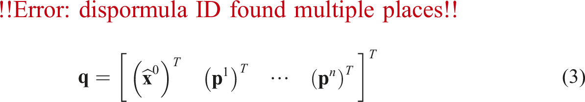
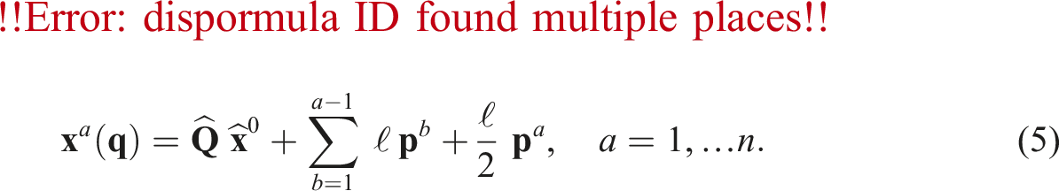
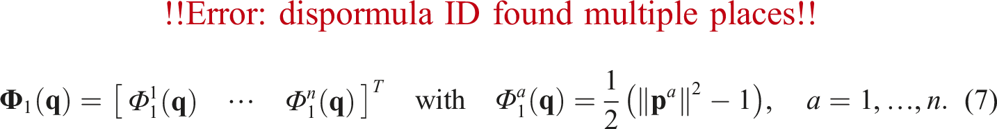
We consider a curved fiber of length L and diameter D, which we model as a polygonal chain with n congruent spherocylinders, i.e., cylinders with hemispherical ends.^38,39 Hence, each segment has a segment length of ℓ = L/n. For the parametrization of such a polygonal chain, following Lauff et al., ³⁹ we normalize the starting point x⁰ of a fiber

${\widehat{\mathbf{x}}}^0={\widehat{\mathbf{Q}}}^{-1}{\mathbf{x}}^0\text{with\hspace{0.17em}the\hspace{0.17em}matrix}\widehat{\mathbf{Q}}=\mathtt{d}\mathtt{i}\mathtt{a}\mathtt{g}(Q_1,Q_2,Q_3),$

(2)comprising the cell dimensions Q _i (i = 1, 2, 3). Then, a fiber may be parametrized via the coordinate vector

$\mathbf{q}={\left[\begin{array}{cccc}\hfill {\left({\widehat{\mathbf{x}}}^0\right)}^{\mathrm{T}}\hfill & \hfill {\left({\mathbf{p}}^1\right)}^{\mathrm{T}}\hfill & \hfill \cdots \hfill & \hfill {\left({\mathbf{p}}^n\right)}^{\mathrm{T}}\hfill \end{array}\right]}^{\mathrm{T}}$

(3)with dimension

$n_q=3(n+1),$

(4)where the unit vectors p ^a ∈ S² (a = 1, …, n) denote the directions of the individual segments. For an illustration of the core idea of the used discretization, see Figure 1. The considered fiber is modeled with n = 5 segments and parametrized via its starting point and the five directions of its segments. With the coordinate vector q, the midpoints of the segments may be expressed explicitly in the form

${\mathbf{x}}^a\left(\mathbf{q}\right)=\widehat{\mathbf{Q}}{\widehat{\mathbf{x}}}^0+\sum _{b=1}^{a-1}\ell {\mathbf{p}}^b+\frac{\ell }{2}{\mathbf{p}}^a,a=1,\dots n.$

(5)As the directions p ^a are assumed to be unit vectors, the configuration space is described by the set

$\mathcal{R}=\left\{\mathbf{q}\in {\mathbb{R}}^{n_q}\left|{\mathbf{\Phi }}_1\left(\mathbf{q}\right)=\mathbf{0}\right.\right\}$

(6)with the n-dimensional vector-valued constraint function

${\mathbf{\Phi }}_1\left(\mathbf{q}\right)={\left[\begin{array}{ccc}\hfill {\Phi }_1^1\left(\mathbf{q}\right)\hfill & \hfill \cdots \hfill & \hfill {\Phi }_1^n\left(\mathbf{q}\right)\hfill \end{array}\right]}^{\mathsf{T}}\text{with}{\Phi }_1^a\left(\mathbf{q}\right)=\frac{1}{2}\left(\Vert {\mathbf{p}}^a{\Vert }^2-1\right),a=1,\dots ,n.$

(7)The configuration space in equation (6) describes fibers residing in the Euclidean space ${\mathbb{R}}^3$ without further restrictions on their location. Also for periodic unit cells, the description in equation (6) is applicable with little extra effort, see Lauff et al. ³⁹ An example for a two-dimensional periodic unit cell with fibers as inclusions is shown in Figure 2. However, when considering fibers with restrictions on their location, i.e., due to the layered structure of a continuous-discontinuous fiber reinforced polymer (CoDicoFRP), the configuration space in equation (6) needs to be adapted according to the underlying box constraints.

Figure 1.

Discretization of a curved fiber as a polygonal chain.

Figure 2.

Fibers in a two-dimensional periodic unit cell.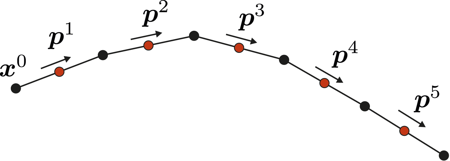

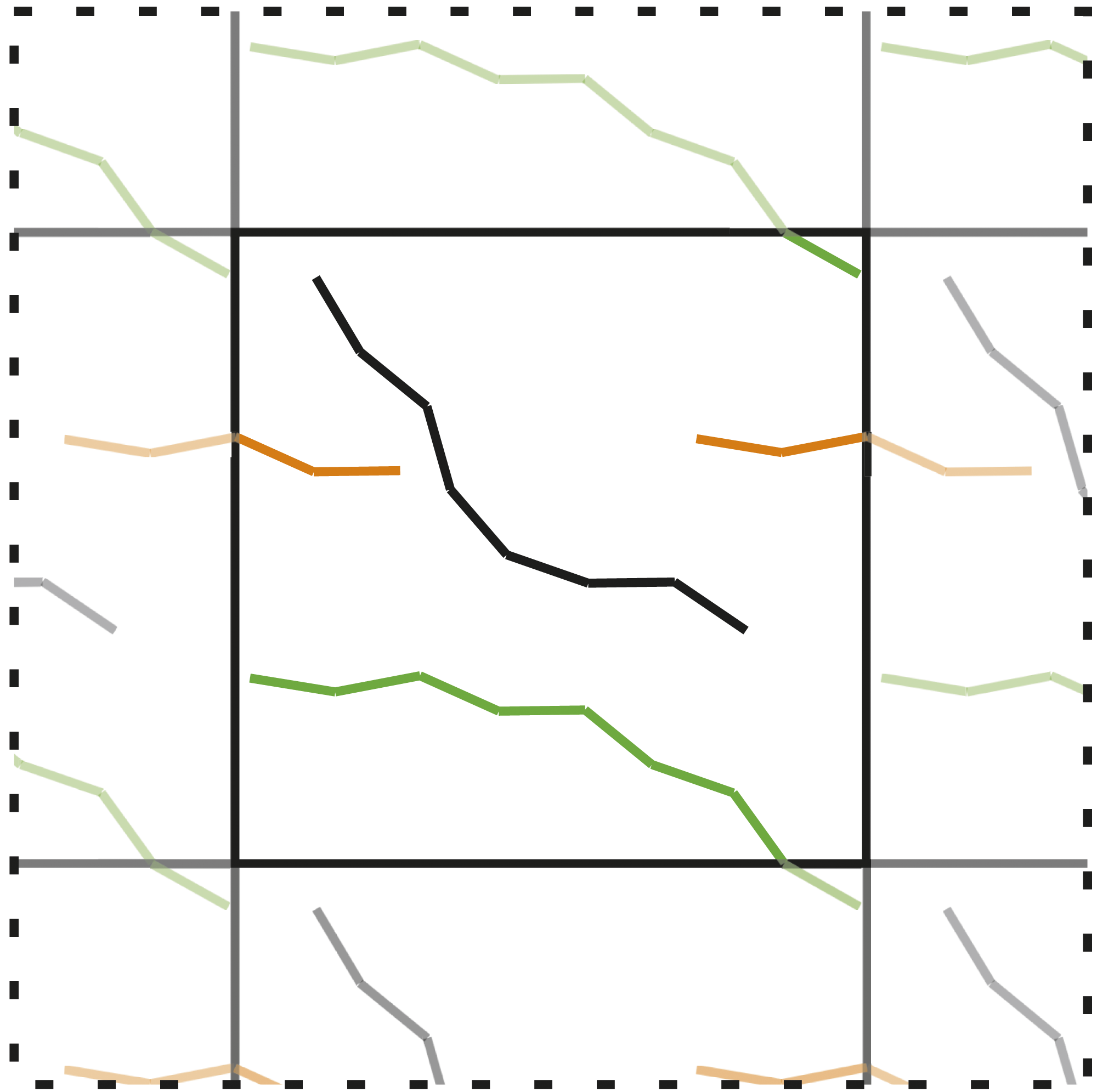
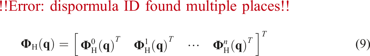
In this manuscript, we aim to consider hard and soft box constraints. In case of hard box constraints, an entire fiber is restricted to its respective cell

$C=\left[B_1,T_1\right]\times \left[B_2,T_2\right]\times \left[B_3,T_3\right],0\le B_i\le T_i\le Q_i,i=\mathrm{1,2,3},$

(8)e.g., to the bottom or the upper layer of a two-layered CoDicoFRP. An admissible configuration of a fiber within its cell is shown in Figure 3(a). Hard box constraints are enforced by restricting the starting point of a fiber and the endpoints of the individual segments to lie within the unit cell. Such a condition may be formulated via the vectorial constraint function

${\mathbf{\Phi }}_{\text{H}}\left(\mathbf{q}\right)={\left[\begin{array}{cccc}\hfill {{\mathbf{\Phi }}_{\text{H}}^0\left(\mathbf{q}\right)}^{\mathsf{T}}\hfill & \hfill {{\mathbf{\Phi }}_{\text{H}}^1\left(\mathbf{q}\right)}^{\mathsf{T}}\hfill & \hfill \cdots \hfill & \hfill {{\mathbf{\Phi }}_{\text{H}}^n\left(\mathbf{q}\right)}^{\mathsf{T}}\hfill \end{array}\right]}^{\mathsf{T}}$

(9)with

$\begin{array}{cc}\hfill & {\mathbf{\Phi }}_{\text{H}}^0\left(\mathbf{q}\right)=\left[\begin{array}{c}\hfill -{\mathbf{x}}^0\hfill \\ \hfill +{\mathbf{x}}^0\hfill \end{array}\right]+\left[\begin{array}{c}\hfill +B_1\hfill \\ \hfill +B_2\hfill \\ \hfill +B_3\hfill \\ \hfill -T_1\hfill \\ \hfill -T_2\hfill \\ \hfill -T_3\hfill \end{array}\right],{\mathbf{\Phi }}_{\text{H}}^a\left(\mathbf{q}\right)=\left[\begin{array}{c}\hfill -\left({\mathbf{x}}^a\left(\mathbf{q}\right)+\ell {\mathbf{p}}^a/2\right)+\left[\begin{array}{c}\hfill B_1\hfill \\ \hfill B_2\hfill \\ \hfill B_3\hfill \end{array}\right]\hfill \\ \hfill +\left({\mathbf{x}}^a\left(\mathbf{q}\right)+\ell {\mathbf{p}}^a/2\right)-\left[\begin{array}{c}\hfill T_1\hfill \\ \hfill T_2\hfill \\ \hfill T_3\hfill \end{array}\right]\hfill \end{array}\right],a=1,\dots ,n.\hfill \end{array}$

(10)

Figure 3.

Illustrative unit cells with hard box constraints (a), soft box constraints with control parameter n_SBC = 0 (b) and soft box constraints with control parameter n_SBC = 2 (c), where the black dots represent the constrained fiber points.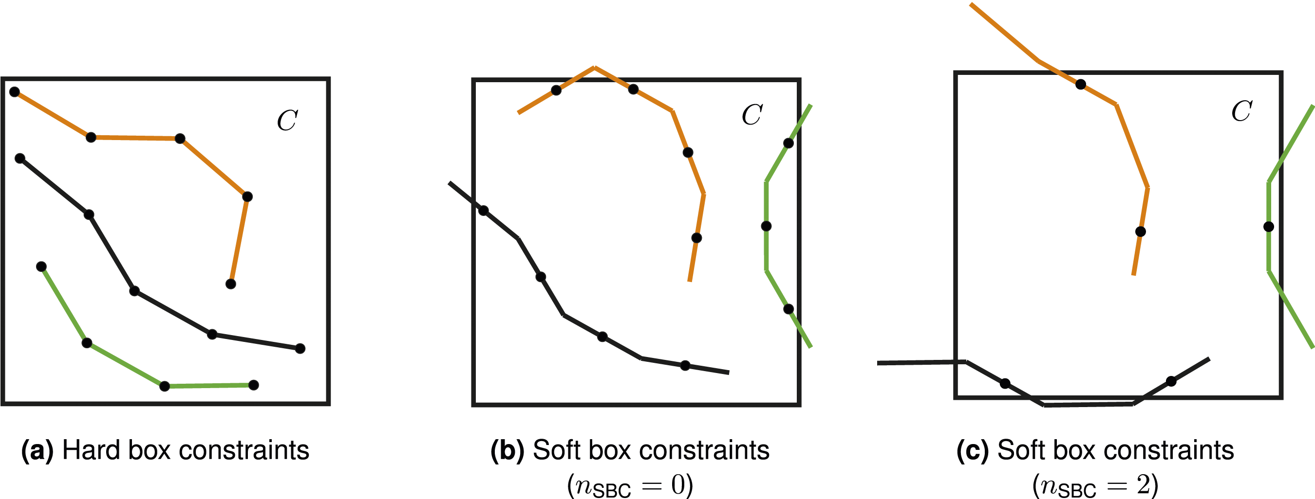

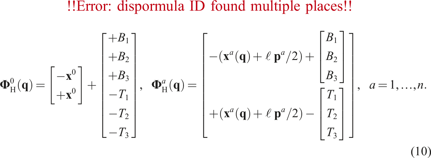
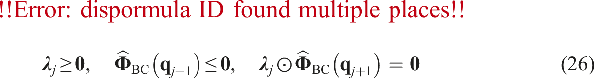
Thus, hard constraints are fulfilled if each component of the vectorial constraint function (9) is smaller or equal than zero.

In case of soft constraints, only the segments’ midpoints of a fiber are restricted to their respective unit cell, see Figure 3(b), and, e.g., an interlocking between two adjacent layers may be realized. Then, the vectorial constraint function is defined by

${\mathbf{\Phi }}_{\text{S}}\left(\mathbf{q}\right)={\left[\begin{array}{ccc}\hfill {{\mathbf{\Phi }}_{\text{S}}^1\left(\mathbf{q}\right)}^{\mathsf{T}}\hfill & \hfill \cdots \hfill & \hfill {{\mathbf{\Phi }}_{\text{S}}^n\left(\mathbf{q}\right)}^{\mathsf{T}}\hfill \end{array}\right]}^{\mathsf{T}}\text{with}{\mathbf{\Phi }}_{\text{S}}^a\left(\mathbf{q}\right)=\left[\begin{array}{c}\hfill -{\mathbf{x}}^a\left(\mathbf{q}\right)+\left[\begin{array}{c}\hfill B_1\hfill \\ \hfill B_2\hfill \\ \hfill B_3\hfill \end{array}\right]\hfill \\ \hfill +{\mathbf{x}}^a\left(\mathbf{q}\right)-\left[\begin{array}{c}\hfill T_1\hfill \\ \hfill T_2\hfill \\ \hfill T_3\hfill \end{array}\right]\hfill \end{array}\right],a=1,\dots ,n.$

(11)

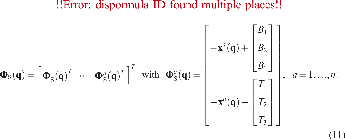
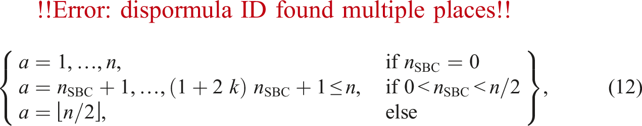
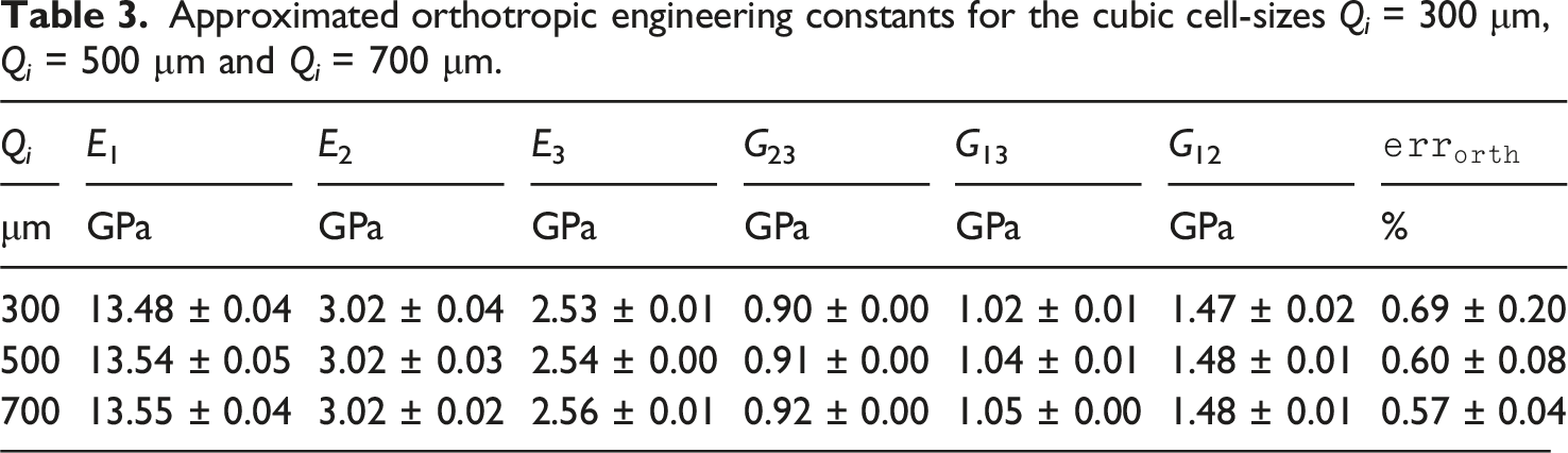
If a fiber is modeled with short segments, most parts of the fiber will not penetrate the cell boundaries. Hence, the difference between hard and soft box constraints decreases for smaller segment lengths. To enable an interlocking also for small segment lengths, we adapt the soft box constraints such that not all midpoints are constrained to their cell, see Figure 3(c). Therefore, we introduce the parameter n_SBC ≥ 0 to control the amount of constrained midpoints. Depending on this parameter, the vectorial constraint function in equation (11) accounts for the midpoints x ^a with

$\left\{\begin{array}{cc}a=1,\dots ,n,\hfill & \text{if\hspace{0.17em}}{n}_{\text{SBC}}=0\hfill \\ a=n_{\text{SBC}}+1,\dots ,(1+2k)n_{\text{SBC}}+1\le n,\hfill & \text{if\hspace{0.17em}}0<n_{\text{SBC}}<n/2\hfill \\ a=\lfloor n/2\rfloor ,\hfill & \text{else}\hfill \end{array}\right\},$

(12)where ⌊⋅⌋ denotes the floor function. Thus, e.g., for a fiber with n = 30 segments, in case of n_SBC = 3 the midpoints x ^a (a = 4, 10, 16, 22, 28) are restricted and in case of n_SBC ≥ 15 only the midpoint x¹⁵ is restricted.

We permit to mix the box-constraint types coordinate-wise, e.g., by using no box constraints for the e ₁-direction, soft box constraints for the e ₂-direction and hard constraints for the e ₃-direction. Hence, the constraint functions (9) and (11) may not be active in all directions and the inactive parts need to be deleted from the formulations. To shorten the expressions, we merge the box constraints to

${\mathbf{\Phi }}_{\text{BC}}\left(\mathbf{q}\right)=\left[\begin{array}{c}\hfill {\mathbf{\Phi }}_{\text{H}}\left(\mathbf{q}\right)\hfill \\ \hfill {\mathbf{\Phi }}_{\text{S}}\left(\mathbf{q}\right)\hfill \end{array}\right]\le \mathbf{0}$

(13)with the dimension n_BC, where the inequality is to be understood component-wise. Then, the configuration space of a curved and constrained fiber is given by the manifold with boundary

${\mathcal{R}}^{\text{BC}}=\left\{\mathbf{q}\in {\mathbb{R}}^{n_q}\left|{\mathbf{\Phi }}_1\left(\mathbf{q}\right)=\mathbf{0},{\mathbf{\Phi }}_{\text{BC}}\left(\mathbf{q}\right)\le \mathbf{0}\right.\right\}.$

(14)

Adapted gradient descent approach on the configuration space of curved and constrained fibers

We consider an objective function

$F:{\mathcal{R}}^{\text{BC}}\to \mathbb{R},\mathbf{q}\mapsto f(\mathbf{q}),$

(15)optimized in the configuration space $\mathbf{q}\in {\mathcal{R}}^{\text{BC}}$ (14). To minimize the objective function, we aim to use a gradient descent approach. However, the standard, i.e., Euclidean, gradient descent method may compute iterates that violate the constraints in equation (14). To ensure an optimization procedure on the optimization space, the gradient descent approach needs to compute iterates along the geodesics, i.e., the locally shortest paths between two points on a manifold. ⁴¹ The equations governing these geodesics follow from minimizing the kinetic energy functional on the manifold, which may be understood as a constrained mechanical system without external forces and driven solely by the kinetic energy.^47,48 For the manifold of a double spherical pendulum, Betsch ⁴⁷ derived the equations governing the geodesics in the form of a d’Alembert type constrained mechanical system. Based on this formulation, Lauff et al. ³⁹ extended the equations for a polygonal chain parametrized via $\mathbf{q}\in \mathcal{R}$ , i.e., without box constraints, which read

$\begin{array}{cc}\hfill {\mathbf{P}(\mathbf{q})}^{\mathsf{T}}\mathbf{G}\ddot{\mathbf{q}}& =\mathbf{0},\hfill \\ \hfill {\mathbf{\Phi }}_1\left(\mathbf{q}\right)& =\mathbf{0}\hfill \end{array}$

(16)with the null space matrix P(q) and the constant symmetric positive-definite metric matrix G. For a detailed derivation of equation (16) and the explicit formulas for the matrices P and G, we refer to Lauff et al. ³⁹ Proceeding from equation (16), the geodesics on the configuration space ${\mathcal{R}}^{\text{BC}}$ may be obtained by enforcing that at each point along the path fulfills the box constraints (13).

With the equations governing the geodesics at hand, we may compute the exponential mapping

${\text{exp}}_{\mathbf{q}}(\mathbf{v})={\mathbf{q}}_v(1)$

(17)for prescribed points $\mathbf{q}\in {\mathcal{R}}^{\text{BC}}$ on the manifold and admissible tangent vectors $\mathbf{v}\in T_{\mathbf{q}}{\mathcal{R}}^{\text{BC}}$ . Here, q _v (1) refers to the endpoint of the geodesic ${\mathbf{q}}_v:[\mathrm{0,1}]\to {\mathcal{R}}^{\text{BC}}$ with the starting point q _v (0) = q and the initial tangent vector ${\dot{\mathbf{q}}}_v(0)=\mathbf{v}$ . Using the exponential mapping to ensure admissible iterates, we adapt the intrinsic gradient descent approach ³⁹ with the iterative procedure

${\mathbf{q}}^{k+1}={\exp }_{{\mathbf{q}}^k}\left(-{\tau }_k{\nabla }_{\mathbf{q}}F({\mathbf{q}}^k)\right),k\in \mathbb{N},$

(18)where τ _k stands for a selected positive stepsize.

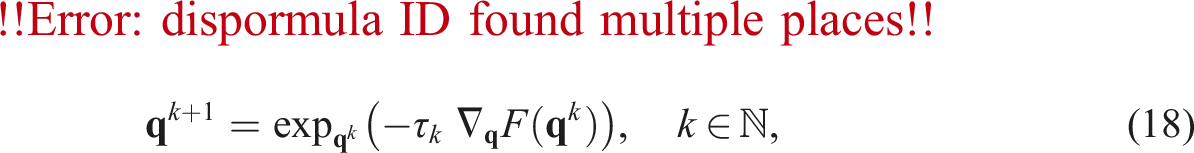
Exponential mapping on the configuration space of curved and constrained fibers

In this section, we introduce a numerical integration scheme for computing the exponential mapping of the manifold with boundary ${\mathcal{R}}^{\text{BC}}$ (17). Following previous publications which consider the exponential mapping of manifolds describing a double spherical pendulum ⁴⁷ and a polygonal chain, ³⁹ we use the energy conserving time integration scheme presented by Gonzales. ⁴⁹

We consider the time interval $I=\left[\mathrm{0,1}\right]$ , which we decompose into n _t subintervals of equal time steps Δt = 1 / n _t . For each subinterval $I_j=\left[t_j,t_{j+1}\right]$ starting at time t _j , the coordinate vector $\mathbf{q}(t)\in {\mathcal{R}}^{\text{BC}}$ and its time derivative $\dot{\mathbf{q}}(t)\in T_{\mathbf{q}}{\mathcal{R}}^{\text{BC}}$ are approximated by the linear approximation formulas

$\begin{array}{c}\hfill \mathbf{q}(t)\approx {\mathbf{q}}_j+\frac{t-t_j}{\mathrm{\Delta }t}\left({\mathbf{q}}_{j+1}-{\mathbf{q}}_j\right),\\ \hfill \dot{\mathbf{q}}(t)\approx {\mathbf{v}}_j+\frac{t-t_j}{\mathrm{\Delta }t}\left({\mathbf{v}}_{j+1}-{\mathbf{v}}_j\right).\end{array}$

(19)With this time discretization scheme, the discretized form of the differential-algebraic equation (16) takes the form

$\begin{array}{c}\hfill {\mathbf{P}\left({\mathbf{q}}_{j+\frac{1}{2}}\right)}^{\mathsf{T}}\widehat{\mathbf{H}}({\mathbf{q}}_j,{\mathbf{q}}_{j+1})=\mathbf{0},\\ \hfill {\mathbf{\Phi }}_1\left({\mathbf{q}}_{j+1}\right)=\mathbf{0}\end{array}$

(20)with the vector-valued function

$\widehat{\mathbf{H}}({\mathbf{q}}_j,{\mathbf{q}}_{j+1})=\frac{2}{\mathrm{\Delta }t}\widehat{\mathbf{G}}\left[{\mathbf{q}}_{j+1}-{\mathbf{q}}_j\right]-2\widehat{\mathbf{G}}{\mathbf{v}}_j$

(21)under the additional inequality constraint accounting for the box constraints (13). The matrix P(q_j+1/2) denotes the null space matrix evaluated for the coordinate vector

${\mathbf{q}}_{j+\frac{1}{2}}=\frac{{\mathbf{q}}_j+{\mathbf{q}}_{j+1}}{2}$

(22)and $\widehat{\mathbf{G}}$ represents the normalized metric matrix

$\begin{array}{cc}\hfill & \widehat{\mathbf{G}}=\left[\begin{array}{ccccc}\hfill {\widehat{\mathbf{Q}}}^{-2}\left[n{\widehat{\mathbf{Q}}}^2\right]\hfill & \hfill {\widehat{\mathbf{Q}}}^{-2}\left[f_1\ell \widehat{\mathbf{Q}}\right]\hfill & \hfill {\widehat{\mathbf{Q}}}^{-2}\left[f_2\ell \widehat{\mathbf{Q}}\right]\hfill & \hfill \cdots \hfill & \hfill {\widehat{\mathbf{Q}}}^{-2}\left[f_n\ell \widehat{\mathbf{Q}}\right]\hfill \\ \hfill \hfill & \hfill {\widehat{\mathbf{Q}}}^{-2}\left[f_{d,1}{\mathbf{1}}_{3\times 3}\right]\hfill & \hfill {\widehat{\mathbf{Q}}}^{-2}\left[f_2{\ell }^2{\mathbf{1}}_{3\times 3}\right]\hfill & \hfill \cdots \hfill & \hfill {\widehat{\mathbf{Q}}}^{-2}\left[f_n{\ell }^2{\mathbf{1}}_{3\times 3}\right]\hfill \\ \hfill \hfill & \hfill \hfill & \hfill \ddots \hfill & \hfill \hfill & \hfill ⋮\hfill \\ \hfill \hfill & \hfill \hfill & \hfill \hfill & \hfill \ddots \hfill & \hfill {\widehat{\mathbf{Q}}}^{-2}\left[f_n{\ell }^2{\mathbf{1}}_{3\times 3}\right]\hfill \\ \hfill \text{sym}\hfill & \hfill \hfill & \hfill \hfill & \hfill \hfill & \hfill {\widehat{\mathbf{Q}}}^{-2}\left[f_{d,n}{\mathbf{1}}_{3\times 3}\right]\hfill \end{array}\right]\hfill \\ \hfill & \text{with}{f}_a=n-a+\frac{1}{2}\text{and}{f}_{d,a}=\epsilon \left(\ell ,D\right)+{\ell }^2\left(n-a+\frac{1}{4}\right),\hfill \end{array}$

(23)where $\epsilon \left(\ell ,D\right)$ denotes the volume-specific moment of inertia of a spherocylinder. ⁵⁰ For more details on the derivation of the discretized differential-algebraic equation (20), we refer to Betsch ⁴⁷ and Lauff et al. ³⁹ The additional inequality constraint accounting for the box constraints (13) leads to the Karush-Kuhn-Tucker (KKT) conditions

$\begin{array}{c}\hfill {\mathbf{P}\left({\mathbf{q}}_{j+\frac{1}{2}}\right)}^{\mathsf{T}}\left[\widehat{\mathbf{H}}({\mathbf{q}}_j,{\mathbf{q}}_{j+1})+{\frac{\partial {\widehat{\mathbf{\Phi }}}_{\text{BC}}\left({\mathbf{q}}_{j+1}\right)}{\partial \mathbf{q}}}^{\mathsf{T}}{\mathit{\lambda }}_j\right]=\mathbf{0},\\ \hfill {\mathbf{\Phi }}_1\left({\mathbf{q}}_{j+1}\right)=\mathbf{0},\\ \hfill {\mathit{\lambda }}_j\ge \mathbf{0},{\widehat{\mathbf{\Phi }}}_{\text{BC}}\left({\mathbf{q}}_{j+1}\right)\le \mathbf{0},{\mathit{\lambda }}_j\odot {\widehat{\mathbf{\Phi }}}_{\text{BC}}\left({\mathbf{q}}_{j+1}\right)=\mathbf{0},\end{array}$

(24)where we use the normalized vectorial constraint function

${\widehat{\mathbf{\Phi }}}_{\text{BC}}\left(\mathbf{q}\right)=\left[\begin{array}{cccc}\hfill {\widehat{\mathbf{Q}}}^{-1}\hfill & \hfill {\mathbf{0}}_{3\times 3}\hfill & \hfill \cdots \hfill & \hfill {\mathbf{0}}_{3\times 3}\hfill \\ \hfill {\mathbf{0}}_{3\times 3}\hfill & \hfill {\widehat{\mathbf{Q}}}^{-1}\hfill & \hfill \cdots \hfill & \hfill {\mathbf{0}}_{3\times 3}\hfill \\ \hfill ⋮\hfill & \hfill ⋮\hfill & \hfill \ddots \hfill & \hfill {\mathbf{0}}_{3\times 3}\hfill \\ \hfill {\mathbf{0}}_{3\times 3}\hfill & \hfill {\mathbf{0}}_{3\times 3}\hfill & \hfill \cdots \hfill & \hfill {\widehat{\mathbf{Q}}}^{-1}\hfill \end{array}\right]{\mathbf{\Phi }}_{\text{BC}}\left(\mathbf{q}\right).$

(25)

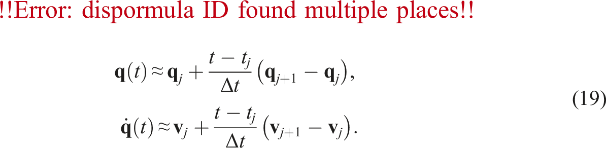
In equation (24), $\mathit{\lambda }\in {\mathbb{R}}^{n_{\text{BC}}}$ denotes the additional vector of unknown Lagrangian multipliers and the notation () ⊙ () represents the element-wise multiplication of two vectors (1). For any fixed parameter vector $\mathit{\mu }\in {\left({\mathbb{R}}^{>0}\right)}^{n_{\text{BC}}}$ , the conditions

${\mathit{\lambda }}_j\ge \mathbf{0},{\widehat{\mathbf{\Phi }}}_{\text{BC}}\left({\mathbf{q}}_{j+1}\right)\le \mathbf{0},{\mathit{\lambda }}_j\odot {\widehat{\mathbf{\Phi }}}_{\text{BC}}\left({\mathbf{q}}_{j+1}\right)=\mathbf{0}$

(26)hold if and only if the equation

${⟨{\mathit{\lambda }}_j+\mathit{\mu }\odot {\widehat{\mathbf{\Phi }}}_{\text{BC}}\left({\mathbf{q}}_{j+1}\right)⟩}_{+}={\mathit{\lambda }}_j$

(27)is satisfied, where ⟨h⟩₊ = max(0, h) denotes the Macaulay bracket, applied component-wise to a vector. Hence, the system of equations and inequalities (24) may be equivalently rewritten as a system of equations

$\begin{array}{c}\hfill {\mathbf{P}\left({\mathbf{q}}_{j+\frac{1}{2}}\right)}^{\mathsf{T}}\left[\widehat{\mathbf{H}}({\mathbf{q}}_j,{\mathbf{q}}_{j+1})+{\frac{\partial {\widehat{\mathbf{\Phi }}}_{\text{BC}}\left({\mathbf{q}}_{j+1}\right)}{\partial \mathbf{q}}}^{\mathsf{T}}{\mathit{\lambda }}_j\right]=\mathbf{0},\\ \hfill {\mathbf{\Phi }}_1\left({\mathbf{q}}_{j+1}\right)=\mathbf{0},\\ \hfill {⟨{\mathit{\lambda }}_j+\mathit{\mu }\odot {\widehat{\mathbf{\Phi }}}_{\text{BC}}\left({\mathbf{q}}_{j+1}\right)⟩}_{+}-{\mathit{\lambda }}_j=\mathbf{0}.\end{array}$

(28)

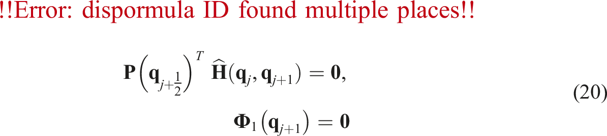
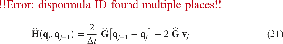
For each subinterval $I_j=\left[t_j,t_{j+1}\right]$ , the coordinate vector ${\mathbf{q}}_j\in {\mathcal{R}}^{\text{BC}}$ and the velocity vector ${\mathbf{v}}_j\in {\mathbb{R}}^{n_q}$ are given quantities at time t = t _j . The coordinate vector q_j+1 is obtained by solving the system of equation (28) with a non-smooth Newton scheme.^44–46 As initial guess for the coordinate vector q_j+1, we choose

${\mathbf{q}}_{j+1}={\mathbf{q}}_j+\mathrm{\Delta }t{\mathbf{v}}_j.$

(29)At convergence of the non-smooth Newton scheme, the velocity vector for the next time step is obtained via

${\mathbf{v}}_{j+1}=\frac{2}{\mathrm{\Delta }t}\left({\mathbf{q}}_{j+1}-{\mathbf{q}}_j\right)-{\mathbf{v}}_j.$

(30)

For the parameter vector μ , we use $\mathit{\mu }=10\cdot {\mathbf{1}}_{n_{\text{BC}}}$ . As convergence criteria of the Newton scheme, we choose that the norm of the residual vector is below 10⁻⁸ and that the inequality constraints are strictly satisfied. Following Lauff et al., ³⁹ we initially consider the complete time interval I with a single time step Δt = 1. If the non-smooth Newton scheme does not converge in ten iterations, we repeat the time integration with doubled subintervals. For Newton’s method applied to find roots of a sufficiently smooth function, backtracking ⁵¹ is a popular strategy to globalize the convergence properties of Newton’s method, which is only characterized by local convergence in its traditional undamped form. For non-smooth problems, however, backtracking is not guaranteed to help upgrading the local convergence behavior of Newton’s method to global convergence. Therefore, backtracking is only used in the case that the inequality constraints are not violated in a time step at all. If backtracking is applied, we use the backtracking parameter β = 0.9, taken from literature. ⁵² Thus, in each backtracking step, the stepsize is moderately reduced by 10%. For the fixed backtracking parameter β = 0.9, we have investigated the influence of the second backtracking parameter $\alpha \in \left(\mathrm{0,0.5}\right)$ on the runtime to solve the system of equation (28). The study has shown that the effect of the parameter α is negligible and we select α = 1/3. To still ensure global convergence of the non-smooth Newton’s method, we rely on a homotopy method, i.e., the previously described adaptive reduction of the time-step size, which permits us to remain in the basin of attraction of the sought root.

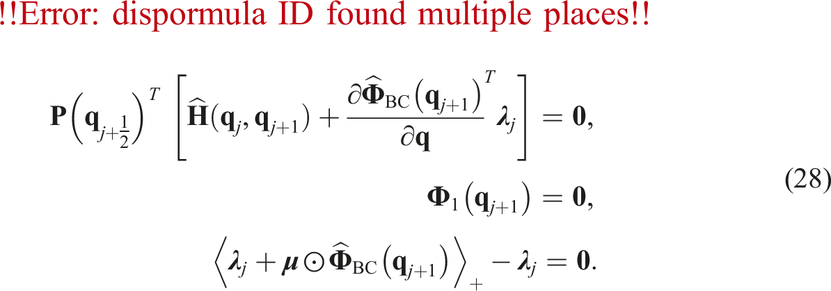
Please note that considering the unknown Lagrangian multipliers in equation (28) increases the dimension of the system equations significantly. Hence, it is important for the performance to consider only those components which are active in the current time step. If a fiber does not touch the boundary of its containing cell, the inequality constraints are considered inactive and should be deleted from the formulation to decrease the dimension and thus the runtime for solving the equations.

Microstructure generation of long fiber reinforced hybrid composites

Description of long fiber reinforced hybrid composites

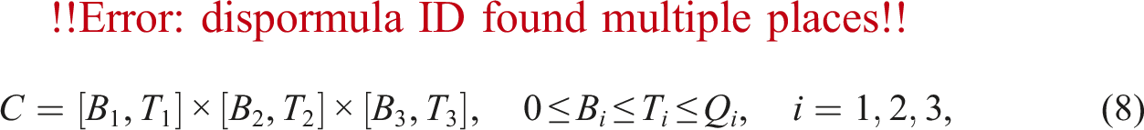
We consider periodic microstructures comprising a rectangular cell $Q=\left[0,Q_1\right]\times \left[0,Q_2\right]\times \left[0,Q_3\right]$ , which is divided into m non-overlapping subcells with rectangular cell dimensions

$C^c=\left[B_1^c,T_1^c\right]\times \left[B_2^c,T_2^c\right]\times \left[B_3^c,T_3^c\right],c=1,\dots ,m.$

(31)Hence, the volume of a subcell computes as

$V_c=\left(T_1^c-B_1^c\right)\left(T_2^c-B_2^c\right)\left(T_3^c-B_3^c\right).$

(32)

In each cell, N _c long, curved fibers of constant diameter D _c without fiber-overlap are given. Thus, the total number of fibers inside the entire unit cell Q equals the sum

$N=\sum _{c=1}^m{N}_c.$

(33)The ordering of the fibers is chosen such that the first N₁ fibers belong to the first cell, the next N₂ fibers to the second cell and so on. The smallest fiber-index corresponding to the c^th-cell is denoted by i _c .

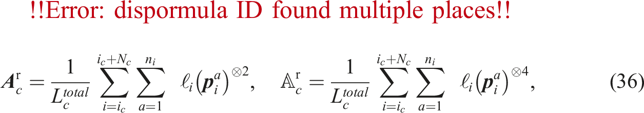
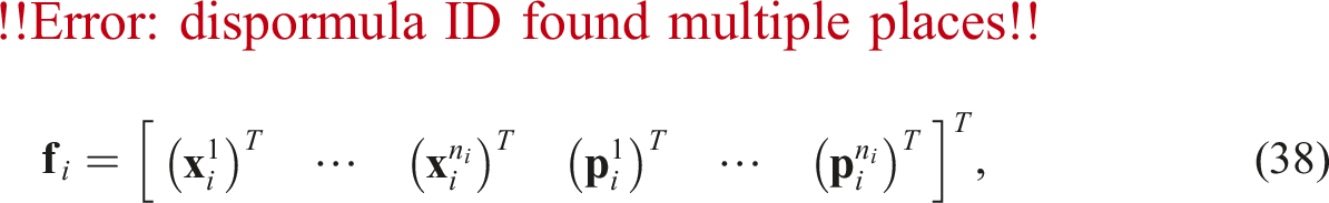
The fibers are modeled as polygonal chains with spherocylindrical segments and are parametrized via the coordinate vector q, see equation (3). The fiber lengths follow a prescribed fiber length distribution, e.g, the uniform, Gamma or Weibull distribution. In this manuscript, we consider cells filled with discontinuous or continuous fibers, where we assume a unidirectional fiber arrangement for the continuous fibers. To model the discontinuous fibers, we select the number of segments of the i^th-fiber such that the segment lengths ℓ _i is below a defined maximum segment length ${\overline{\ell }}_c$

$n_i=\lceil \frac{L_i}{{\overline{\ell }}_c}\rceil ,{\ell }_i=\frac{L_i}{n_i},i=1,\dots ,N,$

(34)where the functional ⌈⋅⌉ computes the smallest integer larger or equal to a given real number. For the continuous and unidirectional fibers, we use a single segment, i.e., we model the fiber as a straight cylindrical geometry.

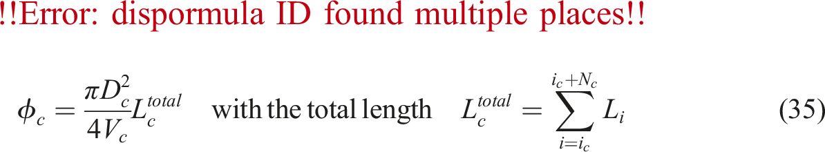
The fiber volume fraction within a subcell computes as

${\varphi }_c=\frac{\pi D_c^2}{4V_c}{L}_c^{total}\text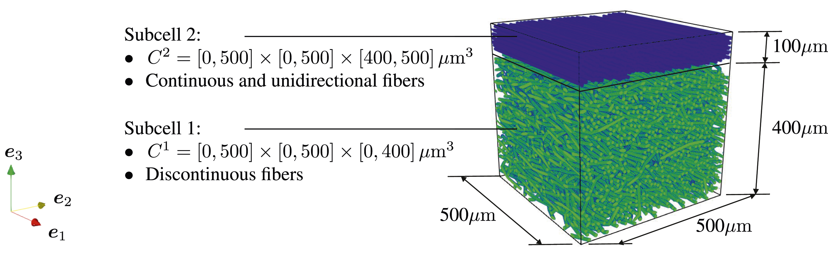{with\hspace{0.17em}the\hspace{0.17em}total\hspace{0.17em}length}{L}_c^{total}=\sum _{i=i_c}^{i_c+N_c}{L}_i$

(35)according to the Pappus’ theorem. ⁵³ The fiber orientation state is typically represented by the fiber orientation tensors,^42,43 where the realized volume-weighted fiber orientation tensors of second ${\mathit{A}}_c^{\text{r}}$ and fourth order ${\mathbb{A}}_c^{\text{r}}$ of each cell compute as

${\mathit{A}}_c^{\text{r}}=\frac{1}{L_c^{total}}\sum _{i=i_c}^{i_c+N_c}\sum _{a=1}^{n_i}{\ell }_i{\left({\mathit{p}}_i^a\right)}^{\otimes 2},{\mathbb{A}}_c^{\text{r}}=\frac{1}{L_c^{total}}\sum _{i=i_c}^{i_c+N_c}\sum _{a=1}^{n_i}{\ell }_i{\left({\mathit{p}}_i^a\right)}^{\otimes 4},$

(36)where the vector ${\mathit{p}}_i^a$ denotes the direction of the a^th-segment of the i^th-fiber. For fiber reinforced composites, the fiber orientation tensor of second order may be identified via micro-CT imaging.^54,55,33 To obtain an adequate approximation of the fiber orientation tensor of fourth order, closure approximation^56–62 may be used. For cells with unidirectional fiber arrangement, e.g., oriented in e ₁-direction, the fiber orientation tensor of second order is given by ${\mathit{A}}_c^{\text{r}}\widehat{=}\mathtt{d}\mathtt{i}\mathtt{a}\mathtt{g}\left(\mathrm{1,0,0}\right)$ . In Figure 4, an example for a hybrid composite with two layers in e ₃-direction is shown. The bottom layer is reinforced with discontinuous fibers and the upper layer is reinforced with continuous fibers in a unidirectional fiber arrangement in e ₁-direction.

Figure 4.

Hybrid composite with two layers in e ₃-direction.

Extension of the fused sequential addition and migration (fSAM) algorithm

In this section, we provide information on the extensions to the original fused sequential addition and migration (fSAM) algorithm ³⁹ to generate periodic hybrid microstructures composed in multiple cells with different prescribed characteristics, e.g., varying fiber length and orientation distributions or fiber volume fractions.

Comment on the fiber orientation term within the objective function

The fSAM algorithm aims to minimize the objective function

$F\left({\mathbf{f}}_1,\dots ,{\mathbf{f}}_N\right)\widehat{=}\frac{1}{2}\sum _{i,j=1}^N\sum _{a=1}^{n_i}\sum _{b=1}^{n_j}{\left({\delta }_{ij}^{ab}\right)}^2+\frac{w_{\mathbb{A}}}{8}N\Vert \mathbb{A}-{\mathbb{A}}^{\text{r}}{\Vert }^2+\frac{w_{\rho }}{2}\sum _{i=1}^N\sum _{a=1}^{n_i-1}{\left({⟨\cos \overline{\alpha }-{\mathit{p}}_i^{a+1}\cdot {\mathit{p}}_i^a⟩}_{+}\right)}^2,$

(37)where the first term accounts for the non-overlap condition between the fiber segments, the second term considers the fiber orientation tensor and the third term restricts the angle between adjacent segments to the maximum angle $\overline{\alpha }$ . For more details on the terms and the weights, we refer to Lauff et al. ³⁹ The coordinate vector f _i denotes an alternative parametrization of a fiber

${\mathbf{f}}_i={\left[\begin{array}{cccccc}\hfill {\left({\mathbf{x}}_i^1\right)}^{\mathsf{T}}\hfill & \hfill \cdots \hfill & \hfill {\left({\mathbf{x}}_i^{n_i}\right)}^{\mathsf{T}}\hfill & \hfill {\left({\mathbf{p}}_i^1\right)}^{\mathsf{T}}\hfill & \hfill \cdots \hfill & \hfill {\left({\mathbf{p}}_i^{n_i}\right)}^{\mathsf{T}}\hfill \end{array}\right]}^{\mathsf{T}},$

(38)which is obtained from the coordinate vector q _i by computing the midpoints of the segments ${\mathbf{x}}_i^a$ , see equation (5).

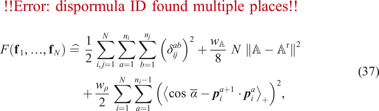
Typically, we prescribe a tolerance for the relative error of the fiber orientation tensor ${ϵ}_{\mathbb{A}}$ as a termination criterion for the optimization problem. However, due to the formulation in equation (37), the fiber orientation will be further corrected during the gradient descent scheme even if the orientation error is below the tolerance, but the other criteria are not fulfilled. As the fiber orientation term leads to non-zero gradients of the objective function for all fiber directions, it is necessary to numerically integrate the d’Alembert constrained mechanical system for all fibers. Thus, the fiber orientation term may result in the computation of the exponential mapping for fibers which already satisfy the maximum angle condition and do not intersect with other fibers, although the fiber orientation tensor is already satisfying its convergence criterion. As a result, the runtime increases significantly, especially at the end of the optimization procedure, as the fiber orientation condition converges first most of the time. To decrease the runtime, we formulate the objective function

$F_{{⟨\cdot ⟩}_{+}}\left({\mathbf{f}}_1,\dots ,{\mathbf{f}}_N\right)\widehat{=}\frac{1}{2}\sum _{i,j=1}^N\sum _{a=1}^{n_i}\sum _{b=1}^{n_j}{\left({\delta }_{ij}^{ab}\right)}^2+\frac{w_{\mathbb{A}}}{8}N{⟨\Vert \mathbb{A}-{\mathbb{A}}^{\text{r}}{\Vert }^2-{ϵ}_{\mathbb{A}}⟩}_{+}+\frac{w_{\rho }}{2}\sum _{i=1}^N\sum _{a=1}^{n_i-1}{\left({⟨\cos \overline{\alpha }-{\mathit{p}}_i^{a+1}\cdot {\mathit{p}}_i^a⟩}_{+}\right)}^2$

(39)such that the term for the fiber orientation tensor is only be considered if the orientation error exceeds the prescribed tolerance ${ϵ}_{\mathbb{A}}$ .

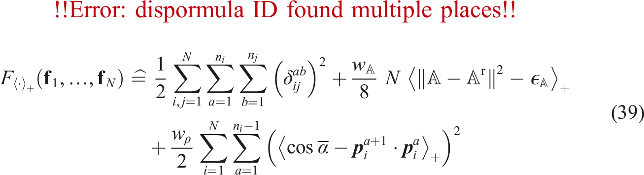
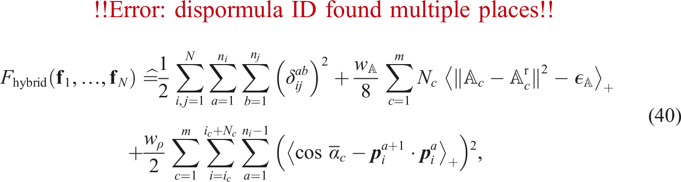
Extension of the objective function for multiple subcells with different characteristics

The objective function in equation (39) only accounts for a single fiber orientation distribution and a uniform maximum angle within the entire cell. As we aim to consider m subcells with different characteristics, we need to distinguish between these areas. Hence, the objective function in equation (37) turns to

$\begin{array}{c}{F}_{\text{hybrid}}\left({\mathbf{f}}_1,\dots ,{\mathbf{f}}_N\right)\widehat{=}\frac{1}{2}\sum _{i,j=1}^N\sum _{a=1}^{n_i}\sum _{b=1}^{n_j}{\left({\delta }_{ij}^{ab}\right)}^2+\frac{w_{\mathbb{A}}}{8}\sum _{c=1}^m{N}_c{⟨\Vert {\mathbb{A}}_c-{\mathbb{A}}_c^{\text{r}}{\Vert }^2-{ϵ}_{\mathbb{A}}⟩}_{+}\\ +\frac{w_{\rho }}{2}\sum _{c=1}^m\sum _{i=i_c}^{i_c+N_c}\sum _{a=1}^{n_i-1}{\left({⟨\cos {\overline{\alpha }}_c-{\mathit{p}}_i^{a+1}\cdot {\mathit{p}}_i^a⟩}_{+}\right)}^2,\end{array}$

(40)where ${\mathbb{A}}_c$ denotes the desired fiber orientation tensor of fourth order of the c^th-subcell and ${\overline{\alpha }}_c$ the maximum angle of the c^th-subcell. The term for the non-overlap condition does not distinguish between different subcells, as the fibers may reach into adjacent subcells, depending on their box constraints. Thus, fibers of different subcells may intersect during the optimization procedure which is not admissible for convergence.

Implementation of soft and hard box constraints

Let us discuss the implementation of the soft and hard box constraints as part of the fSAM algorithm. Therefore, we consider two different procedures. On the one hand, the box constraints may be fulfilled in every iterative step, which we call the intrinsic approach. Then, the gradient steps are restricted on the adapted configuration space of the fibers ${\mathcal{R}}^{\text{BC}}$ , see equation (14). Hence, moving along the geodesics of this manifold requires the numerical integration of the d’Alembert type constrained mechanical system in equation (16) under the condition that the box constraints (13) are fulfilled. In our investigations, it turned out that the term for the fiber orientation tensor converges slowly if fibers are close to their boundaries. Thus, we increase the weight of this term for all fibers which violate the inequality conditions during the previous numerical integration of the d’Alembert constrained mechanical system by a factor of 2.5.

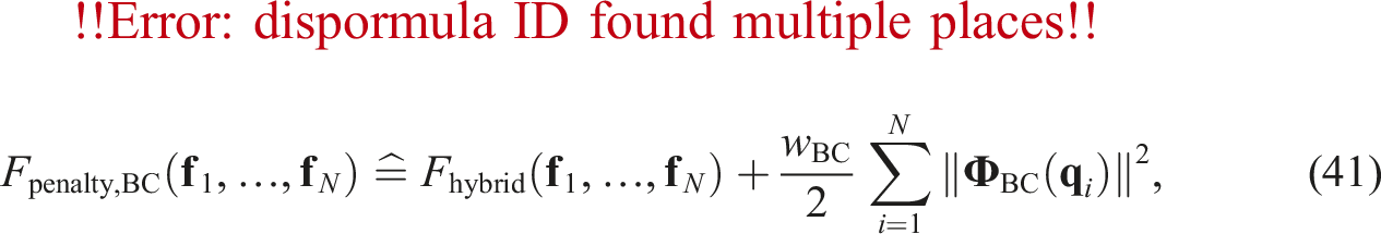
Alternatively, the box constraints may only be enforced via the convergence criterion of the optimization problem, but not in every iterative step. Hence, we consider the d’Alembert type constrained mechanical system in equation (16) without the box constraints during the exponential mapping. To enforce the box constraints, we extend the objective function by a term accounting for the soft and hard box constraints

$F_{\text{penalty,BC}}\left({\mathbf{f}}_1,\dots ,{\mathbf{f}}_N\right)\widehat{=}{F}_{\text{hybrid}}\left({\mathbf{f}}_1,\dots ,{\mathbf{f}}_N\right)+\frac{w_{\text{BC}}}{2}\sum _{i=1}^N{‖{\mathbf{\Phi }}_{\text{BC}}\left({\mathbf{q}}_i\right)‖}^2,$

(41)where the coordinate vector q _i is computed from the coordinate vector f _i . For this change of fiber parametrization, the normalized starting point computes as

${\widehat{\mathbf{x}}}_i^0\left({\mathbf{f}}_i\right)={\widehat{\mathbf{Q}}}^{-1}\left({\mathbf{x}}_i^1-\frac{{\ell }_i}{2}{\mathbf{p}}_i^1\right).$

(42)The objective function $F_{\text{penalty,BC}}\left({\mathbf{f}}_1,\dots ,{\mathbf{f}}_N\right)$ has dimension (length)². Hence, the weight of the box constraints term w_BC needs to be dimensionless and we select w_BC = 5. Due to the additional penalty term within the objective function, we call this procedure the penalty approach.

Sampling and pre-optimization step

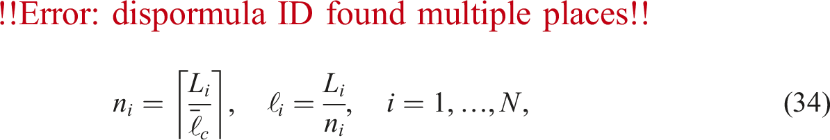
Before the main optimization problem is solved, a sampling step is conducted. Therefore, we first sample fiber lengths according to the prescribed fiber length distribution of each cell until the desired fiber volume fraction is reached. Then, we sample the midpoints and the directions of the fibers, assuming straight fibers first. Therefore, we follow Schneider, ³⁸ by sampling the midpoints from a uniform distribution within the subcells and by sampling the directions from the ACG closure,^63,64 accounting for the prescribed fiber orientation tensors of second order. Subsequently, the segment number of each fiber is determined, see equation (34), and the fibers decompose into segments without changing their location in the cell.

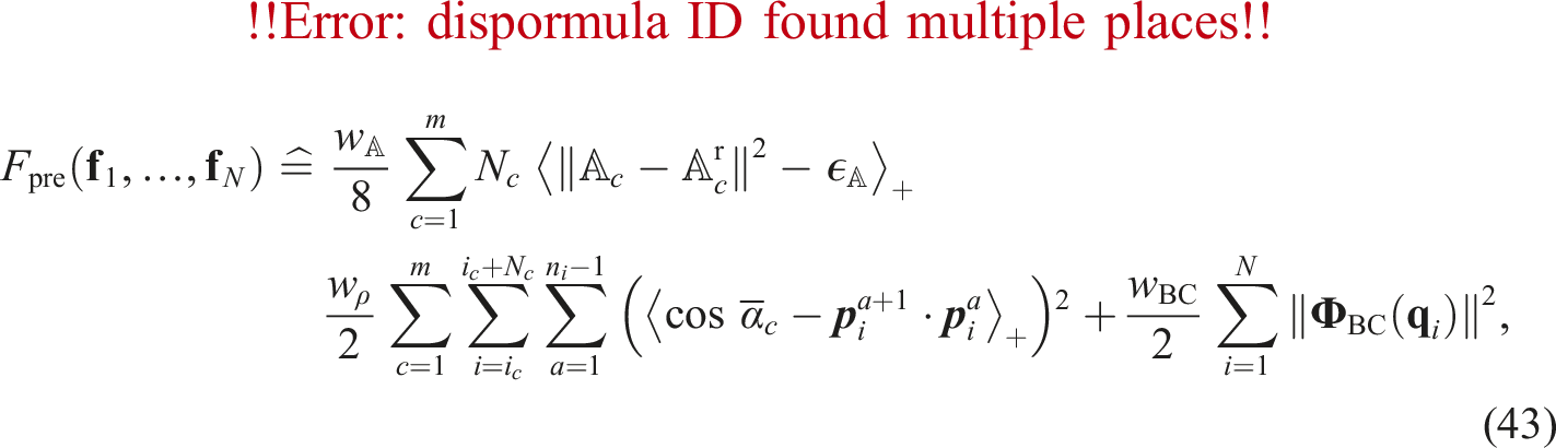
Due to the sampling procedure, the realized fiber orientation tensors may differ from the desired ones. Additionally, the fibers may violate their box constraints, as only the fiber’s midpoints are surely located within their respective cell. To stabilize the convergence behavior of the algorithm, we aim to ensure that the initial fiber orientation tensor of the main optimization problem is within the prescribed tolerance. Furthermore, moving along a geodesic requires the starting configuration to be admissible, i.e., to lie on the manifold of curved and constrained fibers. To obtain a starting configuration for the main optimization according to these requirements, we consider a pre-optimization step subsequent to the sampling step. Therefore, we solve an optimization problem with the objective function

$\begin{array}{c}{F}_{\text{pre}}\left({\mathbf{f}}_1,\dots ,{\mathbf{f}}_N\right)\widehat{=}\frac{w_{\mathbb{A}}}{8}\sum _{c=1}^m{N}_c{⟨\Vert {\mathbb{A}}_c-{\mathbb{A}}_c^{\text{r}}{\Vert }^2-{ϵ}_{\mathbb{A}}⟩}_{+}\frac{w_{\rho }}{2}\sum _{c=1}^m\sum _{i=i_c}^{i_c+N_c}\sum _{a=1}^{n_i-1}{\left({⟨\cos {\overline{\alpha }}_c-{\mathit{p}}_i^{a+1}\cdot {\mathit{p}}_i^a⟩}_{+}\right)}^2\\ & +\frac{w_{\text{BC}}}{2}\sum _{i=1}^N{||{\mathbf{\Phi }}_{\text{BC}}\left({\mathbf{q}}_i\right)||}^2,\end{array}$

(43)which coincides with the objective function of the penalty approach, see equation (41), except for the term of the non-overlap condition. For the weights, we follow the main optimization problem, except for the weight of term for the box constraints w_BC = 0.5. Solving the optimization problem in equation (43) results in a fiber arrangement with accurate fiber orientation realization where the fibers are in admissible configurations on the spaces ${\mathcal{R}}_i^{\text{BC}}$ , but may be overlapping.

Handling of the continuous and unidirectional fibers

Continuous and unidirectional fibers are modeled with a single straight cylindrical segment, which is arranged in one of the three coordinate directions e _i . The segment has the length of the parallel edge of its cell $\left(T_i^c-B_i^c\right)$ . Due to this special resulting configuration, the ends of the segments are in touch when periodically repeating the subcell in fiber direction. Hence, the fiber is continuous.

The fSAM algorithm ²⁴ prescribes a minimum distance to avoid stress peaks between close fibers. Additionally, a self-intersection scheme ³² is used to detect long fibers intersecting themselves. Thus, the algorithm would detect self-intersections for the continuous fibers, although they shall touch at their end. To overcome this limitation, the self-intersection scheme is turned off for continuous fibers.

For subcells reinforced with continuous fibers, we prescribe a unidirectional fiber orientation state. Hence, we know that all segment directions need to be unidirectional for convergence. Thus, we do not change the fiber directions within the main optimization problem. To find a fiber arrangement with no fiber overlap, only the midpoints of the fibers are changed.

Computational investigations

Setup

We use an implementation of the fSAM algorithm written in Python with Cython extensions, where the collision checks between the segments and the numerical integration of the exponential mapping are parallelized with OpenMP. The runtimes were measured on a desktop computer with a 8-core Intel i7 CPU and 64 GB RAM.

As our reference setup, we work with a two-layered CoDicoFRP comprising a discontinuously fiber-reinforced bottom layer and a continuously fiber-reinforced upper layer. For both subcells, we consider a polypropylene (PP) matrix reinforced by E-glass fibers. Table 1 records the corresponding elastic moduli.^65,66 The fiber diameter is assumed to be D = 10 μm for all fibers. For the discontinuous phase, the fibers are modeled with a uniform fiber length of L = 1500 μm, i.e., a fiber aspect ratio of 150, the maximum segment length is set to $\overline{\ell }=50\mathrm{\mu }\mathrm{m}$ and the maximum angle is chosen as $\overline{\alpha }=60°$ . Between all fibers, we ensure a minimum distance of 20% of the fiber diameter, i.e., 2.0 μm.

Table 1.

Material properties for the PP matrix and the E-glass fibers.^65,66

E-glass fibers	PP matrix
E = 72.0 GPa	E = 1.25 GPa
ν = 0.22	ν = 0.35

The fiber orientation tensor of fourth order is obtained by a closure approximation from a prescribed fiber orientation tensor of second order. As we use the exact closure^63,64 and fiber orientation tensors of second order are orthotropic, in general, the fiber orientation tensors of fourth order are orthotropic as well. ⁶⁷ For the convergence of the optimization procedure of the fSAM algorithm, it is necessary that no fiber overlap is detected. Additionally, the relative error in the fiber orientation tensor of fourth order needs to be below 10⁻⁴ and the absolute error of the angle constraint is enforced to be below 10⁻². For the penalty approach, we enforce that the constrained fiber points exceed their boundaries 10⁻³D at most.

To compute the effective elastic properties, we use an FFT-based computational homogenization software^68,69 with a discretization on a staggered grid ⁷⁰ and a conjugate gradient solver.^71,72 As termination criterion for the solver, we choose a relative tolerance of 10⁻⁵. The effective elasticity tensor is computed using six independent load cases. Based on the effective elastic stiffness, we approximate the effective orthotropic engineering constants^73,74 due to the orthotropic material symmetry of the microstructures.

On the algorithmic handling of the box constraints

In this section, we compare the intrinsic and the penalty approach enforcing the box constraints. Therefore, we generate two-layered microstructures with a cubic unit cell and cell dimensions Q _i = 500 μm. The bottom layer with discontinuous fiber-reinforcement has cell dimension 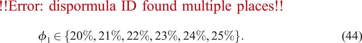$C^1=\left[\mathrm{0,500}\right]\times \left[\mathrm{0,500}\right]\times \left[\mathrm{0,400}\right]\mathrm{\mu }{\mathrm{m}}^{\mathrm{3}}$ and we consider the fiber volume fractions

${\varphi }_1\in \{20\%,21\%,22\%,23\%,24\%,25\%\}.$

(44)We prescribe the fiber orientation tensor of second order ${\mathit{A}}_1\widehat{=}\mathtt{d}\mathtt{i}\mathtt{a}\mathtt{g}\left(0.77,0.17,0.06\right)$ , experimentally measured for long fiber reinforced thermoplastics. ⁷⁵ The upper layer with continuous and unidirectional fiber-reinforcement has cell dimension $C^2=\left[\mathrm{0,500}\right]\times \left[\mathrm{0,500}\right]\times \left[\mathrm{400,500}\right]\mathrm{\mu }{\mathrm{m}}^{\mathrm{3}}$ and a fiber volume fraction of ϕ₂ = 35%. The principal direction of the continuous fibers is the e ₁-direction. For both layers, we consider no box constraints for the e ₁-direction and e ₂-direction. Hence, the fibers may wrap around the unit cell due to the periodic boundary conditions. For the e ₃-direction, we apply hard constraints at height 0 μm and 500 μm, as well as soft box constraints at height 400 μm. A generated microstructure is shown in Figure 4.

For each fiber volume fraction and procedure, we consider ten generated microstructures and report on the measured runtimes in Figure 5. We observe an increase in runtime for packings with higher fiber volume fractions. For the lowest fiber volume fractions ϕ₁ ∈ {20%, 21%}, both procedures have similar runtimes, e.g., the penalty procedure generates microstructures with ϕ₁ = 21% in about 43s on average. However, for higher fiber volume fractions the runtime of the intrinsic approach is always below the runtime of the penalty approach. Additionally, the penalty approach has outliers with extremely high runtimes. For the fiber volume fractions 22%, 23%, 24% and 25%, the intrinsic approach is 1.23, 1.33, 2.26 and 2.21 times faster than the penalty approach, when including the outliers to this consideration.

Figure 5.

Runtimes for the microstructure generation using an approach with intrinsic box constraints control or via a penalty term.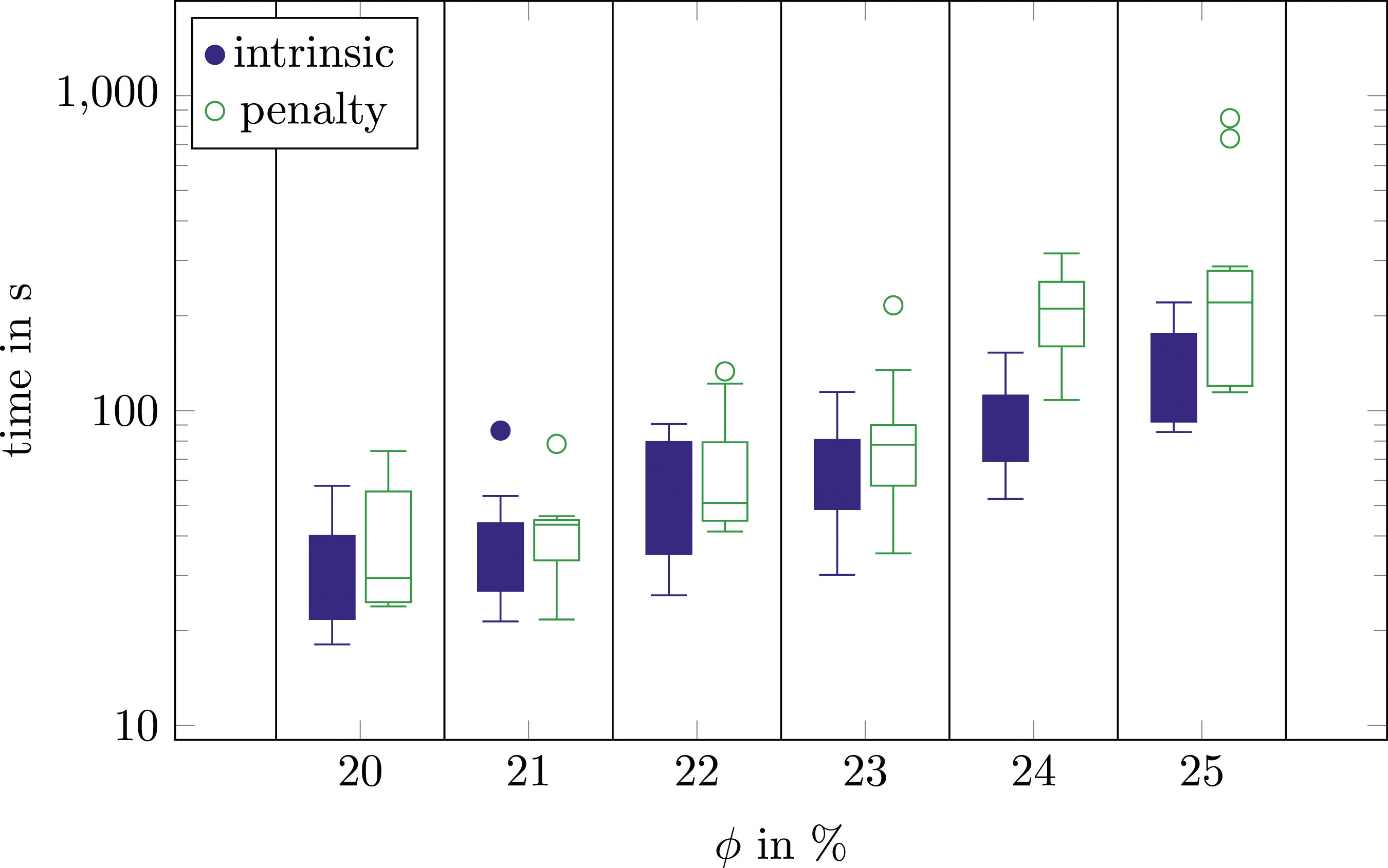

Let us focus on the packing with the highest fiber volume fraction of ϕ₁ = 25% to have a detailed look on the runtimes. For this case, the minimum measured runtime is 86s for the intrinsic approach and 114s for the penalty approach. The maximal measured runtime is 221s for the intrinsic approach and 849s for the penalty approach. Hence, we observe that the minimum runtime observed for both approaches is rather close. However, this is not the case for the maximal runtime as the penalty approach suffers from extreme outliers. For both approaches, the variability in runtime mainly depends on the starting configuration of the fibers, which results from both the sampling and the pre-optimization step. If the starting configuration is challenging with respect to the main optimization problem, e.g., due to a high number of collisions or high angles between the segments, the runtime will increase. Whereas the intrinsic approach is capable of dealing with challenging starting configurations, the penalty approach suffers from convergence problems, especially with increasing complexity, e.g., higher fiber volume fractions. However, still the penalty approach leads to reasonable runtimes for the microstructure generation. Due to the better performance of the intrinsic approach, we will use this procedure for the following investigations.

Resolution study

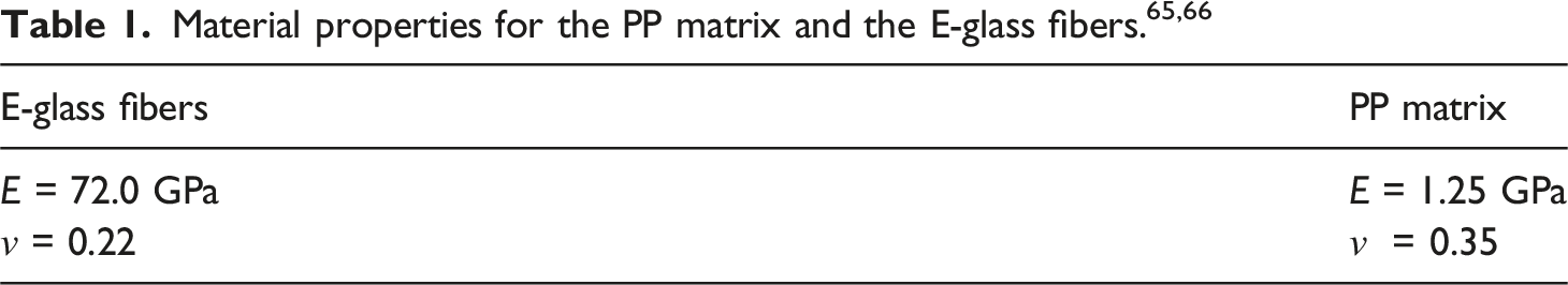
To predict the effective properties with FFT-based computational homogenization methods, a mesh size needs to be chosen which is sufficiently fine to enable an accurate prediction of the effective properties.^72,76 For the resolution study, we consider the setup from the previous subsection with the fiber volume fraction ϕ₁ = 25% and material parameters from Table 1. The cubic cell with cell dimensions Q _i = 500 μm turns out to be representative, see Table 3. To select an adequate mesh size, we compute the effective properties for the four voxel edge-lengths h = 4.00 μm, 2.00 μm, 1.25 μm and 1.00 μm. Compared to the fiber diameter D = 10 μm, a fiber is resolved with 2.5, 5, 8, 10 voxels for decreasing mesh size. As the effort of the homogenization increases with the total voxel number, the finest mesh size with 500³, i.e., 125 ⋅ 10⁶, voxels lead to a significantly higher runtime than the coarsest mesh size with 125³, i.e., about 2 ⋅ 10⁶, voxels. In Figure 6, the same microstructure resolved with the different voxel-edge lengths h = 4.00 μm and h = 1.25 μm is shown.

Figure 6.

Two-layered microstructures resolved with the voxel edge-lengths h = 4.00 μm (a) and h = 1.25 μm (b).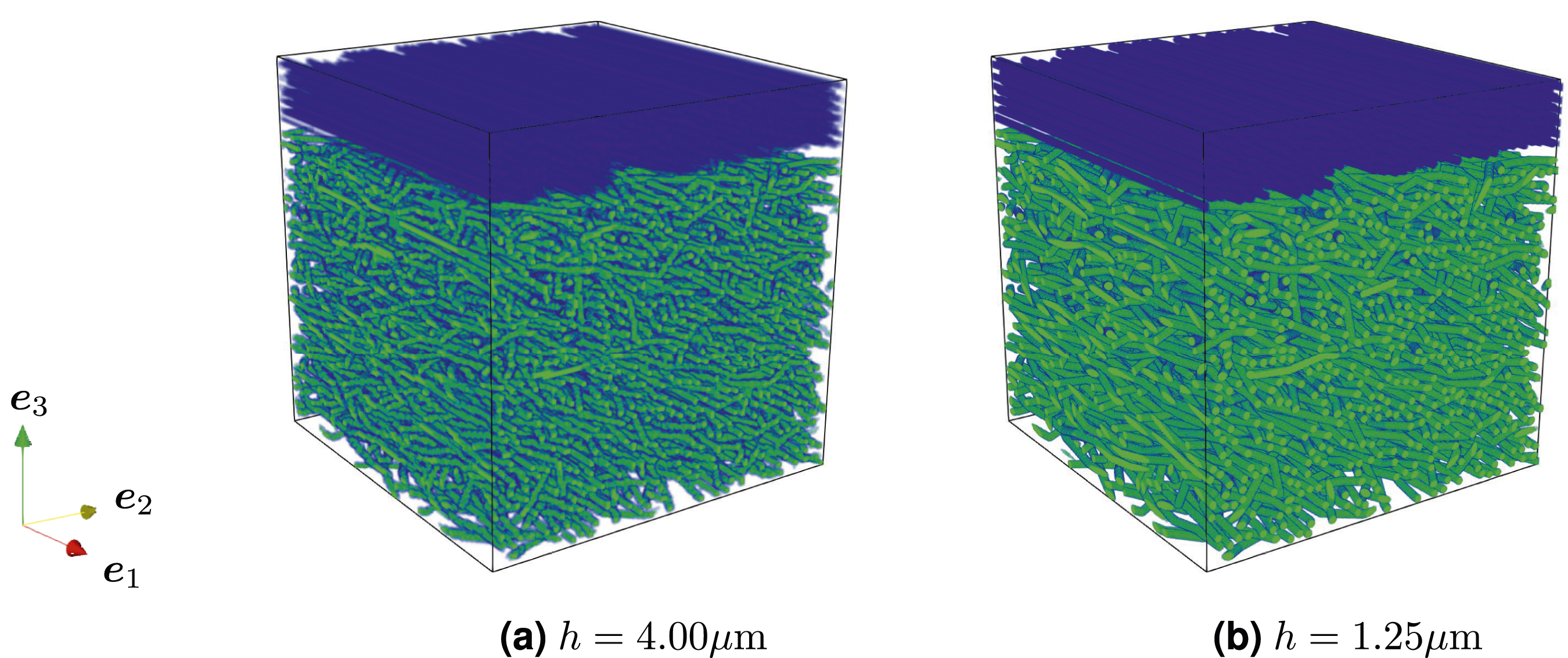

We report on the approximated orthotropic engineering constants for all four voxel-edge lengths in Table 2. To assess the quality of the orthotropic approximation, also the orthotropic approximation error is listed. For the two coarsest mesh sizes, the orthotropic approximation error is 2.76% and 1.07%, dropping below 1% for the two finer mesh sizes. Hence, it turns out that the approximation of the orthotropic engineering constants is adequate. Due to the fiber-reinforcement in e ₁-direction of the upper layer and the preferred fiber arrangement in e ₁-direction of the bottom layer, the Young’s modulus E₁ exceeds the remaining Young’s moduli by multiples. To select a sufficiently fine mesh size, we compare the elastic moduli of the three coarser mesh sizes to the finest mesh size. For the shear modulus G₁₃, the highest relative difference is measured with 16.50% for the coarsest mesh size, reducing to 4.85% and 0.97% for the two finer mesh sizes. As the computed orthotropic approximation error and the resolution induced error is below 1% for the voxel-edge length h = 1.25 μm, we select this voxel-edge length as our mesh size.

Table 2.

Approximated orthotropic engineering constants for the voxel edge-lengths h = 4.00 μm, h = 2.00 μm, h = 1.25 μm and h = 1.00 μm.

h	E 1	E 2	E 3	G 23	G 13	G 12	${\mathtt{e}\mathtt{r}\mathtt{r}}_{\mathtt{o}\mathtt{r}\mathtt{t}\mathtt{h}}$
μm	GPa	GPa	GPa	GPa	GPa	GPa	%
4.00	12.53	3.13	2.76	1.03	1.20	1.62	2.76
2.00	13.32	3.02	2.57	0.94	1.08	1.49	1.07
1.25	13.53	3.00	2.54	0.91	1.04	1.47	0.56
1.00	13.60	3.00	2.53	0.90	1.03	1.46	0.44

RVE study

For computational homogenization of random materials, the selected unit cell size is of key importance to ensure representativity. Due to practical reasons the unit cell needs to be finite, and the apparent effective properties of random materials include a certain degree of randomness as well. However, to obtain the effective properties as deterministic descriptors, the unit cell size needs to be large enough to cover the entire material statistics and ensure that the boundary conditions do not impact the results.^77,78 Such a unit cell is called representative volume element (RVE). As the computational effort for the homogenization depends on the unit cell size, the smallest possible RVE size should be selected.

To assess the representativity of a unit cell, two errors need to be monitored.^14,79 On the one hand, the random error, or dispersion, measures the variability of the realized apparent properties for a fixed unit cell size, i.e., may be monitored by the standard deviation of multiple realizations. On the other hand, the systematic error, or bias, quantifies the difference between the mean apparent properties and the effective properties. Typically, the effective properties are not known. However, to quantify the systematic error, the mean apparent properties of increasing unit cell sizes may be monitored.

For the RVE study, we work with the two-layered microstructure already used in the previous two sections. To study the representativity of different unit cell sizes, we consider cubic cells with cell dimensions Q _i = 300 μm, 500 μm and 700 μm, where the boundary between the two layers is always at height 0.8 Q₃, i.e., at 240 μm, 300 μm and 560 μm, respectively, for increasing cell dimensions. To ensure a sufficiently fine resolution, we use a voxel edge-length of h = 1.25 μm, according to the resolution study in Table 2. Thus, 240³, i.e., about 14 ⋅ 10⁶, voxels resolve the smallest unit cell and 560³, i.e., 176 ⋅ 10⁶, resolve the largest unit cell. For each unit cell size, a generated microstructure is shown in Figure 7. To investigate the representativity errors, we consider ten microstructures for each unit cell size. The mean and the standard deviation of the approximated engineering constants are listed in Table 3. We observe that the orthotropic approximation is suitable for all three unit cell sizes as the error is always below 1%. Also, the standard deviation is low for all unit cell sizes. For the systematic error, we report the highest relative error for the smallest unit cell size Q _i = 300 μm and the shear modulus G₁₃ with 2.86%, dropping to 0.95% for the unit cell size Q _i = 500 μm. Hence, even the smallest unit cell size has rather small representativity errors. To ensure that both the systematic and the random error are well below 1%, we select the unit cell size with cell dimensions Q _i = 500 μm for the further investigations.

Figure 7.

Generated microstructures for three different cubic cell-sizes Q _i .

Table 3.

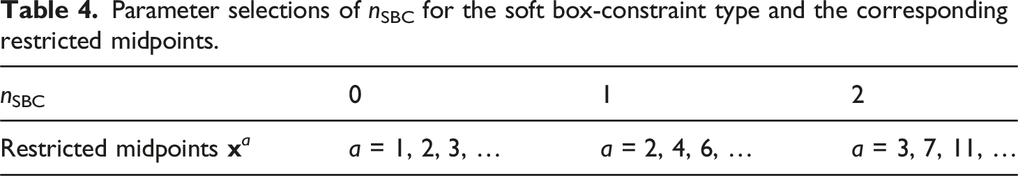
Approximated orthotropic engineering constants for the cubic cell-sizes Q _i = 300 μm, Q _i = 500 μm and Q _i = 700 μm.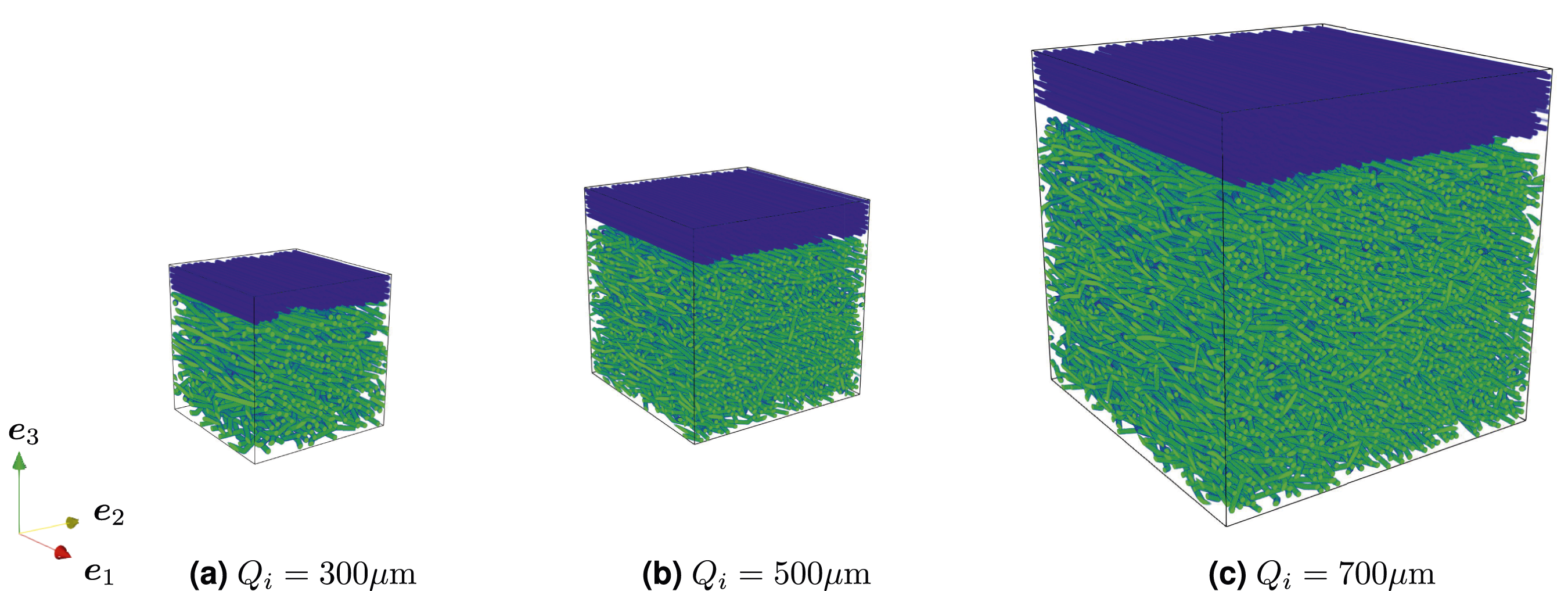

Q i	E 1	E 2	E 3	G 23	G 13	G 12	${\mathtt{e}\mathtt{r}\mathtt{r}}_{\mathtt{o}\mathtt{r}\mathtt{t}\mathtt{h}}$
μm	GPa	GPa	GPa	GPa	GPa	GPa	%
300	13.48 ± 0.04	3.02 ± 0.04	2.53 ± 0.01	0.90 ± 0.00	1.02 ± 0.01	1.47 ± 0.02	0.69 ± 0.20
500	13.54 ± 0.05	3.02 ± 0.03	2.54 ± 0.00	0.91 ± 0.00	1.04 ± 0.01	1.48 ± 0.01	0.60 ± 0.08
700	13.55 ± 0.04	3.02 ± 0.02	2.56 ± 0.01	0.92 ± 0.00	1.05 ± 0.00	1.48 ± 0.01	0.57 ± 0.04

We remark that the fSAM algorithm generates periodic microstructures, regardless which box constraints are applied to the fibers. Already in previous publications^38,24 it is emphasized that periodic microstructures with accurately realized characteristics, i.e., the fiber volume fraction or the fiber orientation tensor of fourth order, combined with periodic boundary conditions for the displacement field during the homogenization are advantageous for decreasing the RVE size.

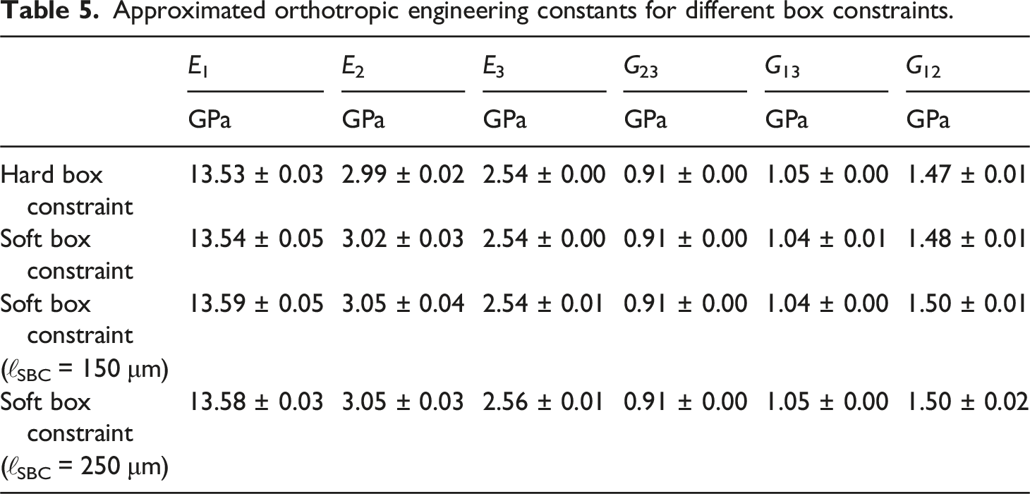
On the difference between soft and hard box constraints

In this section, we study the influence of the selected box constraints on the generated microstructures. Therefore, we work with the two-layered CoDicoFRP already used in the previous sections, see Figure 4, and change the box-constraint type between the bottom and the top layer. For the study, we compare four different box-constraint types. First, we use the hard box constraints, where the complete fiber is enforced to be within its cell. Then, we consider the soft box-constraint type with three different parameter selections of n_SBC, which controls the amount of restricted midpoints. In Table 4, the three considered parameter selections of n_SBC and the corresponding restricted midpoints x ^a are listed.

Table 4.

Parameter selections of n_SBC for the soft box-constraint type and the corresponding restricted midpoints.

n SBC	0	1	2
Restricted midpoints x a	a = 1, 2, 3, …	a = 2, 4, 6, …	a = 3, 7, 11, …

For each box-constraint type, one of the ten generated microstructures is shown in Figure 8. We observe that for the hard box constraint in Figure 8(a) the boundary between the two layers is extremely straight and all fibers are completely in their cell, as enforced. For the soft box constraint with n_SBC = 0, the microstructure in Figure 8(b) looks quite similar. Due to the small maximum segment length of $\overline{\ell }=50\mathrm{\mu }\mathrm{m}$ , the fibers are mainly located in their respective layer and interlocking is suppressed. During the compression molding of CoDicoFRP, the material flow leads to ply migration between the two phases. ⁸⁰ To model such a ply migration, we also consider higher parameter selections of n_SBC, restricting less segment midpoints to their cell, see Table 4. Figure 8(c) shows a microstructure generated with n_SBC = 1. We observe that the discontinuous fibers reach into the adjacent layer. Hence, this parameter selection may be suitable to realize the interlocking of the CoDicoFRP layers. When further increasing the parameter n_SBC to 2, the discontinuous fibers wrap around the continuous fiber-reinforcement, see Figure 8(d). Whereas this is not representative for CoDicoFRP, such a strong connection may appear for other use cases, i.e., the layer boundaries of discontinuous fiber-reinforced materials with a skin-core–skin structure.^81,33,82

Figure 8.

Two-layered continuous-discontinuous fiber-reinforced composite with different box constraints at the layer interface.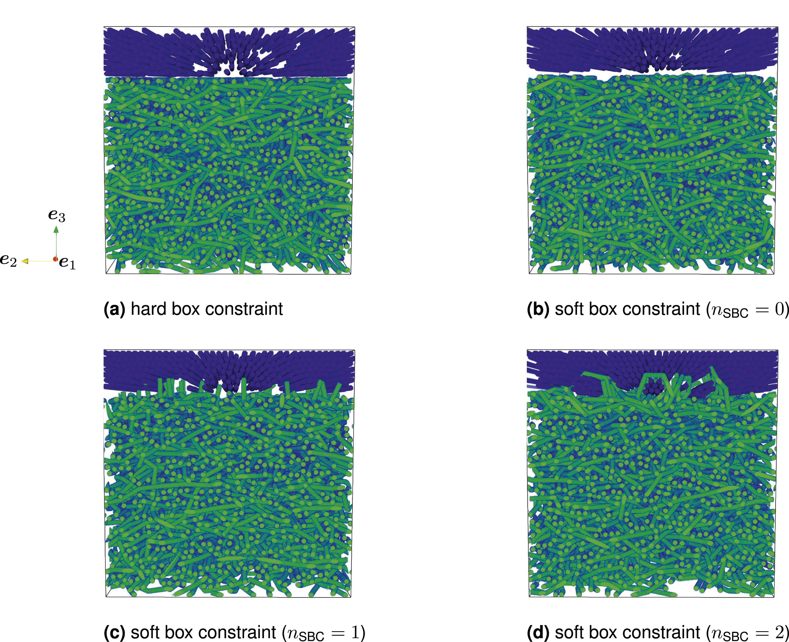

Besides a visual comparison of the generated microstructures, we also study the influence of the box constraints on the effective elastic properties. Therefore, we consider ten microstructures for each box constraint and report on the approximated orthotropic engineering constants in Table 5. It turns out that the effective stiffness increases slightly with higher interlocking, where the differences are rather small and below 1% for all cases. However, the influence of the box constraints may be higher, e.g., when considering the damage behavior of the inter-laminar region.^83,84

Table 5.

Approximated orthotropic engineering constants for different box constraints.

	E 1	E 2	E 3	G 23	G 13	G 12
	GPa	GPa	GPa	GPa	GPa	GPa
Hard box constraint	13.53 ± 0.03	2.99 ± 0.02	2.54 ± 0.00	0.91 ± 0.00	1.05 ± 0.00	1.47 ± 0.01
Soft box constraint	13.54 ± 0.05	3.02 ± 0.03	2.54 ± 0.00	0.91 ± 0.00	1.04 ± 0.01	1.48 ± 0.01
Soft box constraint	13.59 ± 0.05	3.05 ± 0.04	2.54 ± 0.01	0.91 ± 0.00	1.04 ± 0.00	1.50 ± 0.01
(ℓSBC = 150 μm)
Soft box constraint	13.58 ± 0.03	3.05 ± 0.03	2.56 ± 0.01	0.91 ± 0.00	1.05 ± 0.00	1.50 ± 0.02
(ℓSBC = 250 μm)

Comparison to experimental data

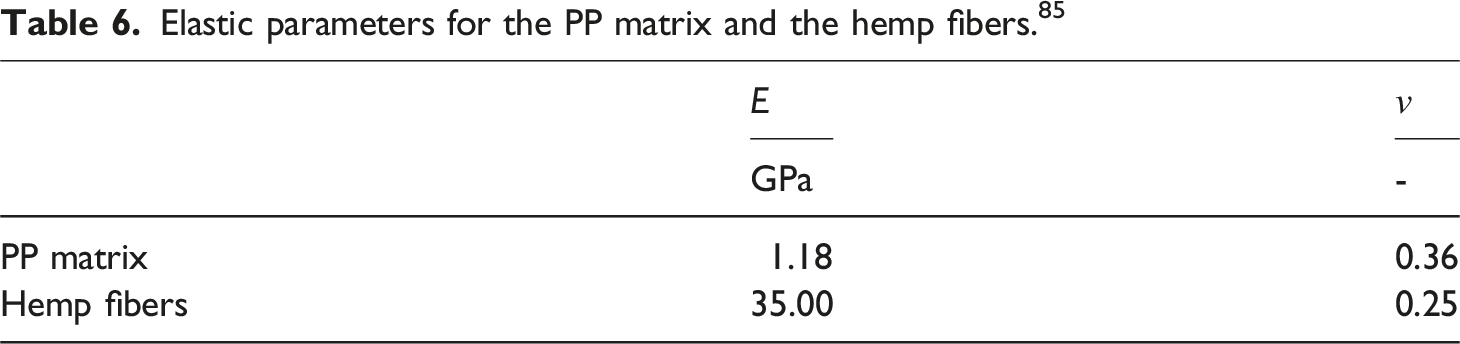
Hemp-fiber reinforced DicoFRP

We start the validation section by comparing the effective properties of microstructures with either straight or curved fibers to experimental data. Therefore, we consider a hemp-fiber reinforced DicoFRP with polypropylene (PP) as the matrix. The elastic parameters of the materials are listed in Table 6. According to Bourgogne, ⁸⁵ the fibers have a diameter of D = 30 μm, come with a fiber length of L = 250 μm and are processed with a fiber volume content of 17.3%. Hence, we consider short fibers with a fiber aspect ratio of r _a ≈ 8.3. Following the suggestion by Bourgogne, ⁸⁵ we use an isotropic fiber orientation state for the considered composite. For the microstructure generation, we enforce a minimum distance between the fibers of 20%, i.e., 6.0 μm, and use a maximum segment length of 40 μm in case of curved fibers. Straight fibers are realized with a single segment per fiber. We select a cubic cell with cell dimensions Q _i = 750 μm and resolve the microstructures with a voxel edge-length of 3.75 μm, i.e., according to the resolution study, eight voxels per diameter. In Figure 9, microstructures with straight and curved fibers are shown. Based on ten realizations, the mean runtime to generate a microstructure with straight fibers is 2s and to generate a microstructure with curved fibers is 19s.

Table 6.

Elastic parameters for the PP matrix and the hemp fibers. ⁸⁵

	E	ν
	GPa	-
PP matrix	1.18	0.36
Hemp fibers	35.00	0.25

Figure 9.

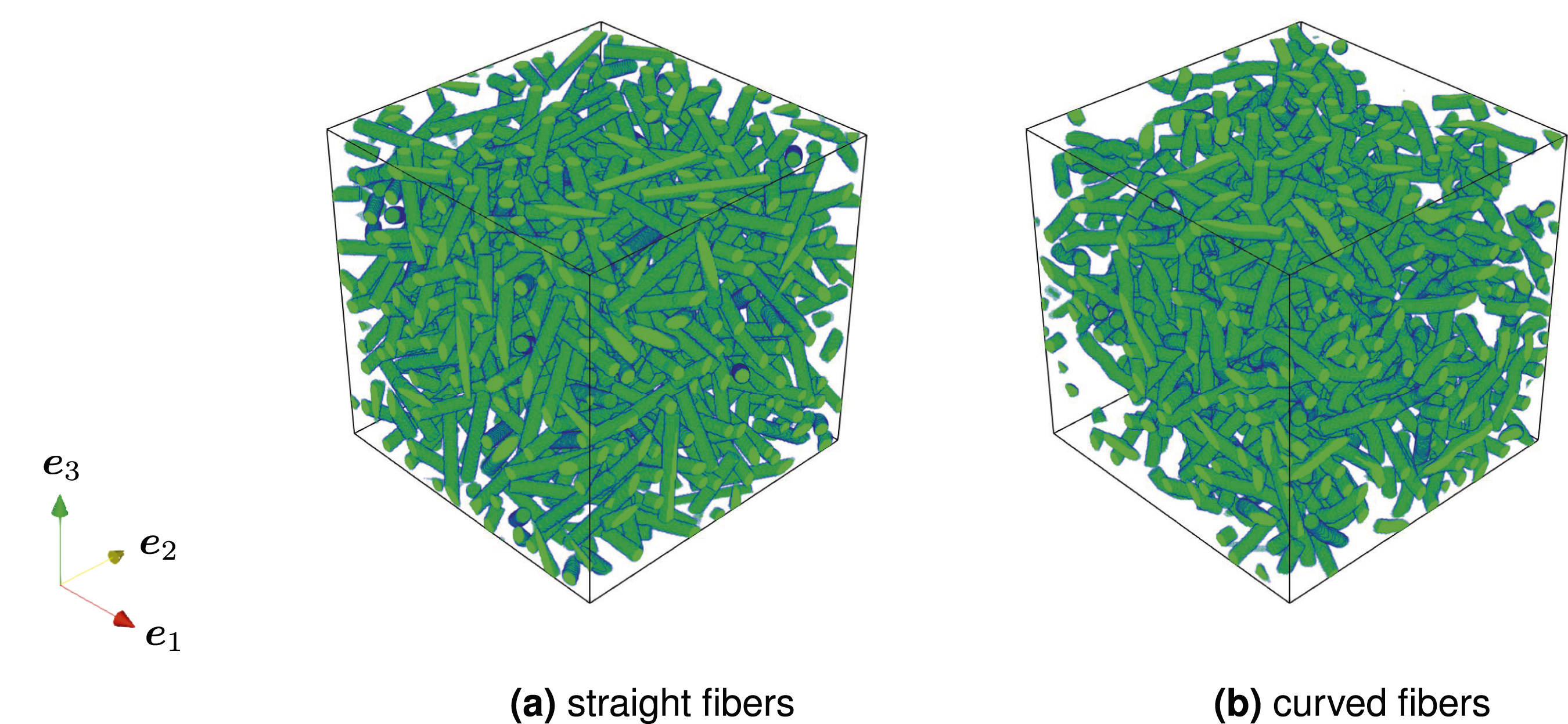
Microstructures with straight (a) and curved (b) fibers.

The experiments ⁸⁵ revealed a Young’s modulus E₁ of about 2.06 GPa for the hemp-fiber reinforced composite. To compare the mechanical behavior of the generated microstructures with the experimental data, we also report on the mean Young’s modulus E₁ obtained from ten realizations. For the microstructures with straight fibers, we obtained a mean Young’s modulus of E₁ = 2.03 GPa and for the curved fibers we obtained a mean Young’s modulus of E₁ = 1.98 GPa. Hence, we observe that the influence of the curvature is rather small with a relative decrease of 2.5% compared to straight fibers. Additionally, the results show a good agreement with the experimental data for both cases.

Carbon-fiber reinforced CoDicoFRP

Besides the hemp-fiber reinforced DicoFRP, we consider a CoDicoFRP with two continuous fiber-reinforced shell layers and a core layer with discontinuous fiber-reinforcement. For the materials, we use a polyamide 6 (PA6) matrix (Technyl^®star, DOMO Chemicals GmbH) reinforced with carbon fibers (PX35, ZOLTEK). The considered elastic parameters for both materials are listed in Table 7. We model the matrix with isotropic material parameters, taking the Young’s modulus E from the data sheet of a commercially available polyamide ⁸⁶ and the Poisson’s ratio ν from the literature. ⁸⁷ For the carbon fibers, we assume a transversely isotropic material symmetry and use the elastic modulus E₁ from the data sheet of the PX35 carbon fibers. ⁸⁸ For the remaining parameters, we use the material data of HTA carbon fibers (Toho Tenax) ⁸⁹ with similar elastic modulus E₁. Fiedler et al. ⁸⁹ report on the orthotropic engineering constants of the HTA carbon fibers. Based on the corresponding orthotropic stiffness, the transversely isotropic engineering constants in Table 7 are obtained by a projection on the transverse isotropic stiffness space.^73,74 The diameter of the carbon fibers is D = 7.2 μm. ⁸⁸

Table 7.

Elastic parameters for the PA6 matrix^86,87 and the carbon fibers.^88,89

	E	ν
	GPa	-
PA6 matrix	3.7	0.4

	E 1	E 2	G 12	ν 23	ν 12
	GPa	GPa	GPa	-	-
Carbon fibers	242	28	32.4	0.23	0.23

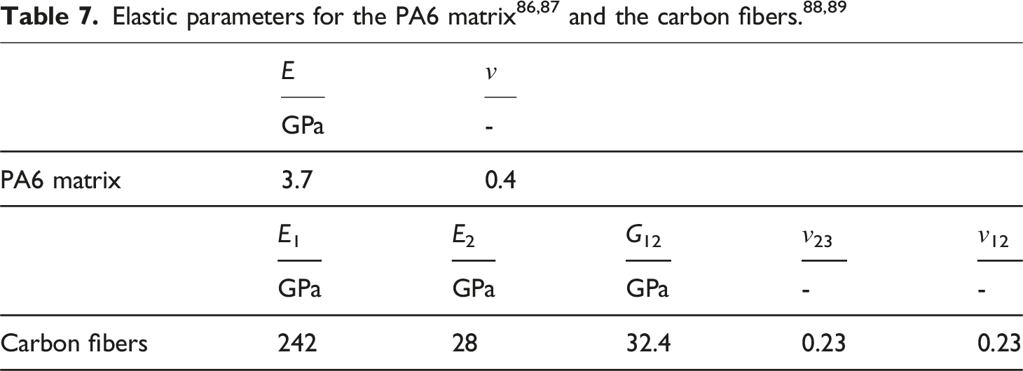
The CoDicoFRP parts were manufactured with the long fiber reinforced thermoplastic direct (LFT-D) compression molding process^90,91 at the Fraunhofer ICT in Pfinztal, Germany, co-molding the LFT plastificate with the continuous and unidirectional fiber-reinforced tapes. The tapes include a fiber mass fraction of 60%, ⁹² i.e., a fiber volume fraction of 48%, and are fiber-reinforced in the flow direction, which is the e ₁-direction. For the Dico material, fiber content and fiber length measurements were conducted at the Fiber Institute Bremen (FIBRE), Germany, see ⁹³ for more details. The fiber volume content measurement revealed a fiber volume fraction of 23.5% on average. With respect to the fiber lengths, a number-weighted mean fiber length of L = 1550 μm and a median value of L = 540 μm was measured. Additionally, the fiber orientation tensors of the Dico material were analyzed and tensile tests for the manufactured CoDicoFRP parts conducted at the IAM, KIT, Germany. For more details on the procedures for the fiber orientation determination and the tensile tests, we refer to Scheuring et al.^75,93 Compression molding leads to parts which may be separated in two areas, depending on the initial charge of the LFT plastificate, the charge and the flow area. For the fiber orientation determination and the tensile tests, at least five samples were taken from both areas. In this investigation, we consider the results of the flow area. The mean fiber orientation tensor of second order is

${\mathit{A}}_{\text{Dico}}\widehat{=}\left[\begin{array}{ccc}\hfill 0.85\hfill & \hfill 0.07\hfill & \hfill 0.00\hfill \\ \hfill 0.07\hfill & \hfill 0.14\hfill & \hfill 0.00\hfill \\ \hfill 0.00\hfill & \hfill 0.00\hfill & \hfill 0.01\hfill \end{array}\right].$

(45)The experimental results for the planar Young’s modulus are shown in Figure 10, where the angle φ represents the deviation from the flow direction. The measuring points

$\phi \in \{0°,22.5°,45°,90°,135°,157.5°\}$

(46)were considered. Due to the continuous fiber-reinforcement in flow direction and the highest eigenvalue a₁ of the fiber orientation tensor (45), the Young’s modulus in flow direction at φ = 0° is the highest modulus with 43.14 GPa. The smallest planar Young’s modulus is at φ = 90° with 7.95 GPa.

Figure 10.

Comparison of the Young’s modulus in the e ₁- e ₂-plane of the CoDicoFRP.

We aim to generate RVEs for the considered CoDicoFRP. Therefore, we select the subcell dimensions

$\begin{array}{cc}\hfill & C^1=\left[\mathrm{0,600}\right]\times \left[\mathrm{0,600}\right]\times \left[\mathrm{0,25}\right]\mathrm{\mu }\mathrm{m},\hfill \\ \hfill & C^2=\left[\mathrm{0,600}\right]\times \left[\mathrm{0,600}\right]\times \left[\mathrm{25,275}\right]\mathrm{\mu }\mathrm{m},\hfill \\ \hfill & C^3=\left[\mathrm{0,600}\right]\times \left[\mathrm{0,600}\right]\times \left[\mathrm{275,300}\right]\mathrm{\mu }\mathrm{m},\hfill \end{array}$

(47)such that the height of the cell (and of the subcells) is ten times smaller than the manufactured parts. According to the manufactured part, we pack the shell layers with a fiber volume fraction of 48% and prescribe a unidirectional fiber arrangement in e ₁-direction. For the core layer, we prescribe the measured fiber volume fraction of 23.5% and the second-order fiber orientation tensor in equation (45). To stay between the measured mean and median fiber length, we use a uniform fiber length of 720 μm, i.e., a fiber aspect ratio of 100. With respect to the algorithmic choices, we use the soft box-constraint type with n_SBC = 1 to model the interface between the subcells. Due to the decreased diameter of D = 7.2 μm, we consider a smaller minimum distance of 1.44 μm. In Figure 11, a synthetic microstructure for a CoDicoFRP is shown, including 1073 fibers with a total number of 11167 segments. For the ten generated microstructures, the mean runtime for the microstructure generation is 156min.

Figure 11.

Synthetic microstructure of a CoDicoFRP using experimentally measured characteristics.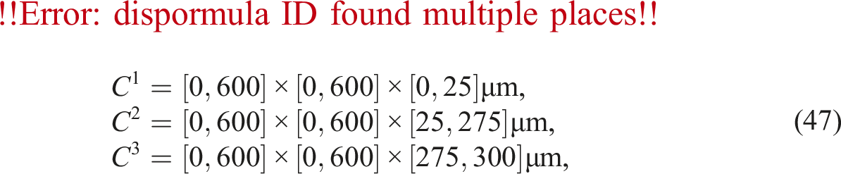

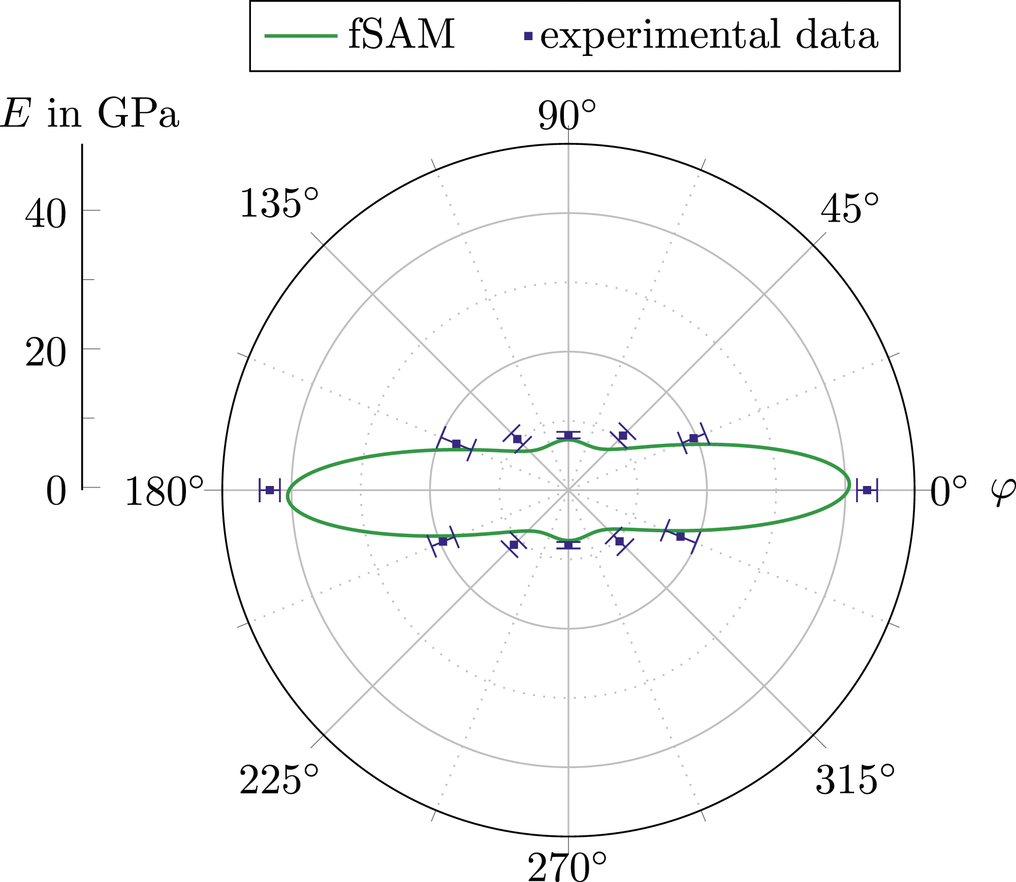
Let us compare the effective stiffness of the synthetic microstructures with the manufactured parts. For the resolution, we use h = 0.8 μm, i.e., the diameter is resolved by 9 voxels and the entire cell consists of 750² × 375 ≈ 211 ⋅ 10⁶ voxels. Based on the computed stiffness of the ten generated microstructures, we compute the direction dependent planar Young’s modulus ⁹⁴ and report on the mean values in Figure 10. We observe that the highest Young’s modulus is not computed at the angle φ = 0° but at the angle φ ≈ 1.5°. This shift results from the compression molding process of the LFT plastificates and is known in the literature.^95,96,75,93 Notice that the generated microstructures are still orthotropic as we prescribe a fiber orientation tensor of second order and use an exact closure^63,64 to obtain the fiber orientation of fourth order. ⁶⁷ However, the considered bases { e ₁, e ₂, e ₃} does not represent the orthotropic axes as the second-order fiber orientation tensor of the Dico phase (45) is not given in its principle axis system, i.e., its matrix-representation is not diagonalized. The orthotropic axis system of the generated microstructures may be obtained with a normal right rotation of the bases { e ₁, e ₂, e ₃} by about 1.5° around the e ₃-axes. Compared to the experimental data, it turns out that the shape of the planar Young’s modulus shows good agreement but the quantitative values are slightly underestimated. For the Young’s modulus at φ = 0°, the computed value is 40.41 GPa, which is a relative difference to the experiments of 6.3%, and at φ = 90°, the computed value is 7.28 GPa, i.e., a relative underestimation of 8.4%.

Summary and conclusion

This manuscript deals with an extension of the fused sequential addition and migration (fSAM) ³⁹ algorithm to generate hybrid composites with long fiber reinforcement. The fSAM algorithm models the fibers as polygonal chains and uses an optimization procedure on the configuration space of a polygonal chain to generate microstructures. To distinguish between different cells of hybrid composites, an adapted configuration space of a polygonal chain is used to account for box constraints, which restrict the location of a fiber to its respective subcell. Depending on the considered material system, the subcells may be strictly separated or interlocked by fibers reaching into adjacent subcells. To enable different interfaces, the fSAM algorithm works with multiple box-constraint types. In case of the hard box constraints, the entire fiber is restricted to its cell, whereas for the soft box constraints only the segment midpoints of a polygonal chain are enforced to be within their cell. Hence, for the latter box constraint, an interlocking between adjacent subcells is enabled. However, when considering small segment lengths, the degree of interlocking is rather small as the fibers are mainly located within their subcell. To ensure interlocking also for decreasing segment lengths, an adapted soft box-constraint type may be selected where only selected segment midpoints are restricted.

Due to the connectivity constraint of a polygonal chain, the optimization problem of the original fSAM algorithm is defined on a curved, i.e., non-flat, configuration space. To compute admissible iterates, an adapted gradient descent approach is used, moving along the geodesics, i.e., the shortest path between two points on the configuration space. To account for the box constraints, the extended fSAM algorithm provides two alternative approaches. On the one hand, the penalty approach uses the original iteration rule which leads to iterates violating the box constraints. To ensure that the solution configuration at convergence is admissible, an additional penalty term accounting for the box constraints is added to the objective function. On the other hand, the intrinsic approach is based on an iteration rule which accounts directly for the box constraints. As the original iteration rule of the fSAM algorithm is only capable of handling equality constraints, a novel strategy is included in this manuscript to move along the geodesics of manifolds whose descriptions include inequality constraints as well, e.g., the box constraints. Hence, each iterate of the intrinsic approach is admissible on the configuration space of a curved and constrained fiber, i.e., a penalty term for the box constraints is not necessary. A detailed derivation of the extended iteration rule is given within the work at hand. For both strategies, the manuscript includes a discussion on the implementation within the framework of the fSAM algorithm. Additionally, information on further adaptions, which are necessary to generate hybrid composites, is provided, concerning the sampling, the pre-optimization step and the adaption of the objective function.

The computational investigations lead to the following findings:

• Due to the faster microstructure generation, the intrinsic approach is advantageous compared to the penalty approach to handle the box constraints. Especially for complex microstructures with high fiber volume fractions, the penalty approach suffers from convergence problems in case of challenging starting configurations, e.g., with many fiber collisions.

• The fSAM algorithm for hybrid composites generates fiber microstructures with high confidence in the desired properties, e.g., the fiber volume fraction or the fiber orientation tensor. Thus, even small unit cell sizes are representative and may be used as RVEs. As the runtime for the microstructure generation and the computational homogenization increases for larger unit cell sizes, the small RVE sizes ensure a computationally efficient prediction of the effective mechanical behavior of the material.

• The shape of the interfaces between adjacent subcells strongly depends on the selected box-constraint type. Whereas the hard box-constraint type leads to a strict separation, the soft box-constraint type enables interlocking, which increases with less restricted segment midpoints. Although the visual comparison results in significant differences, the effective elastic stiffness is in a close range for all implemented box-constraint types. However, the box-constraint type may have a higher influence, e.g., when investigating the damage behavior of the inter-laminar region.

• The microstructures generated by the fSAM algorithm are capable of representing the mechanical behavior of long fiber reinforced hybrid composites. The computed effective stiffness of a synthetic CoDicoFRP with shell-core-shell structure shows a good agreement with experimental measured data. The computed Young’s moduli E₁ and E₂ are 40.41 GPa and 7.28 GPa, slightly underestimating the experimental results with a relative difference of 6.3% and 8.4%, respectively.

To conclude, the studies demonstrate the capability of the extended fSAM algorithm to generate representative volume elements for long fiber reinforced hybrid composites in an efficient manner. Due to the possibility of choosing the box-constraint type, the interface may be modeled according to the considered material system. Hence, either strictly separated areas or interlocked areas can be realized by the microstructure model. With respect to the computational effort of the subsequent homogenization, the fSAM algorithm is a resource-saving method due to the small RVE sizes. By comparing the mechanical behavior of synthetic and manufactured CoDicoFRPs, the novel methodology permits to predict the measured elastic properties with high fidelity.

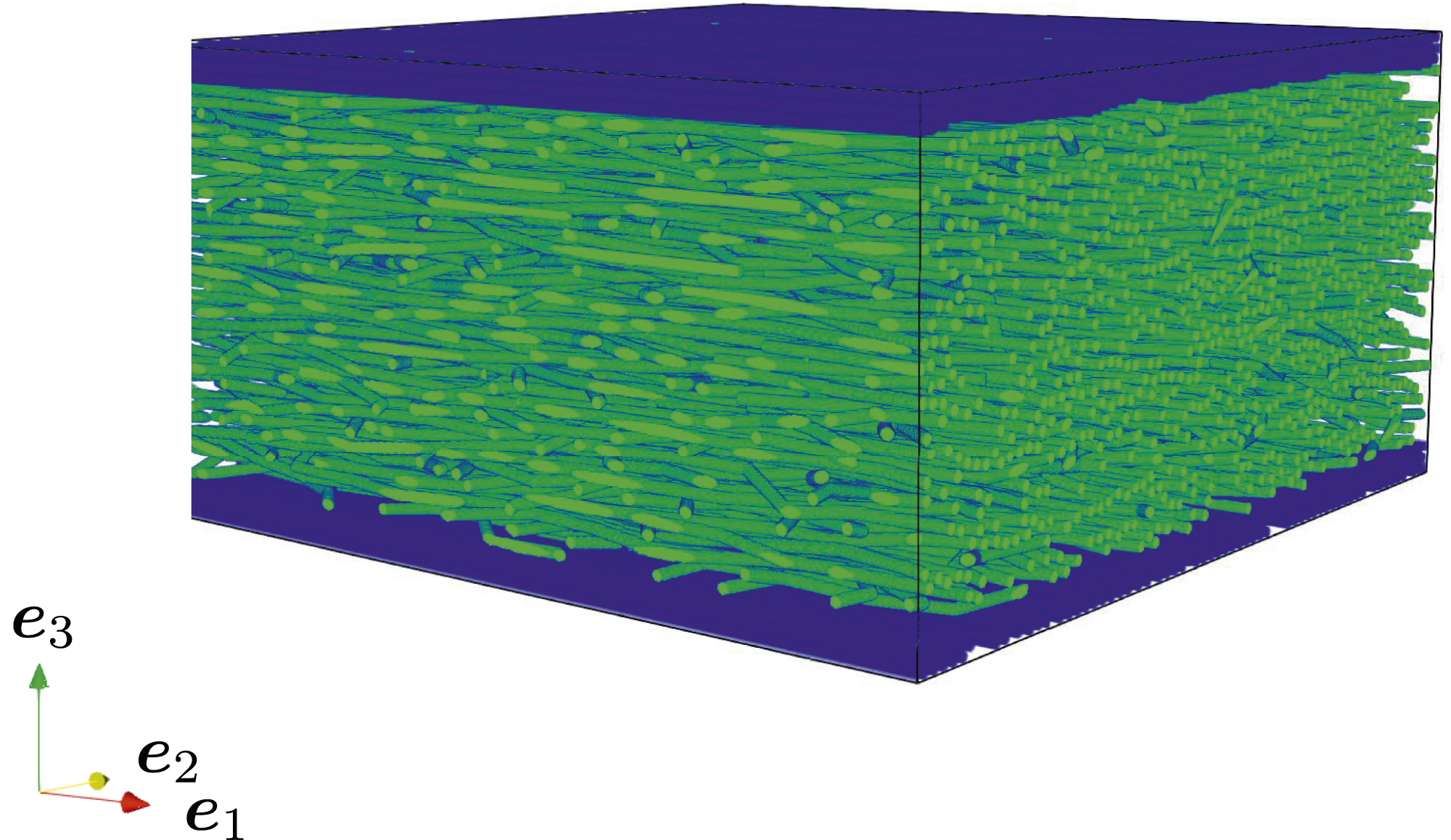
Besides CoDicoFRPs with long, curved fibers, as shown in Figure 12(a), the fSAM algorithm is also applicable to other material systems. Let us give two examples. For CoDicoFRPs with short fibers in the discontinuous fiber-reinforced phase, bending is typically negligible. Thus, the fSAM algorithm generates the corresponding microstructures by modeling the fibers with one cylindrical segment, see Figure 12(b). Another field of application are purely discontinuous fiber-reinforced materials with a skin-core–skin structure,^81,33,82 where the descriptors vary in each layer, see Figure 12(c).

Figure 12.

Three examples for hybrid or multilayer fiber-reinforced composites generated with the fSAM algorithm.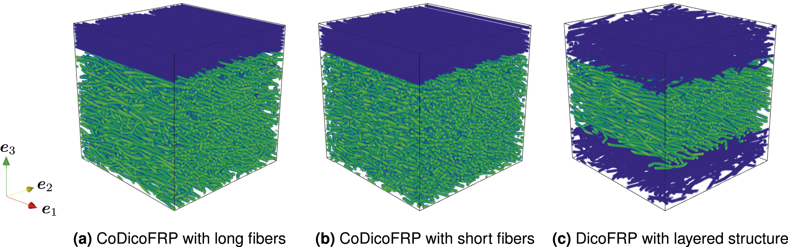

As a future development, one could account for the generation of interphases between the fibers and the matrix material, ⁹⁷ especially when investigating interphase damage. ⁹⁸ Additionally, strategies are necessary to generate microstructures with higher fiber volume fractions and fiber aspect ratios as, e.g., highly aligned fiber-reinforced microstructures are manufactured with fiber volume fractions above 50% and fiber aspect ratios above 500.^99,100 Throughout this manuscript, only the linear elastic material behavior of the composites was investigated. In perspective, it also might be of interest to study the damage behavior^52,83,84 of the generated microstructures and to take the nonlinear thermoviscoelastic behavior of the matrix material ¹⁰¹ into consideration.

As a key feature, the fSAM algorithm models the fibers as flexible structures including curvature. Different studies^{102,38,103,85} report that microstructures with varying degrees of curvature show differences in their mechanical properties. Hence, it is important to study the influence of the fiber curvature on the computed effective stiffness. The fSAM algorithm permits only to decide whether fibers can be curved or not. Prescribing the degree of curvature is not (yet) possible. Additionally, for long fibers, the fiber volume content that can be achieved with straight fibers is extremely limited. Hence, for high fiber aspect ratios and fiber volume fractions, the influence of the curvature cannot be studied at all. To overcome these limitations, it could be part of future research to extend the fSAM algorithm by curvature control such that the influence of the fiber curvature is assessable and the degree of curvature may be prescribed as additional desired characteristic.