Shape recovery of polymers with inclusions under multi-axial stress

Abstract

This paper presents a two-phase composite model for predicting the shape memory and recovery behaviors of polymeric and particle-loaded polymeric composite parts. The shape recovery behavior is simulated using a homogenized material model with the matrix exhibiting the strain storage behavior and the inclusions adding to the stiffness and conductivity of the material. An electrically conductive reinforcement in the matrix enabled the activation of shape recovery with Joule heating. The shape recovery model for the matrix is adapted from literature and extended to include a three-dimensional stress state. Inclusions are assumed linearly elastic, and the matrix is elastic at the low-temperature glassy phase and elastic-incompressible at the high-temperature rubbery phase. The incompressibility is modeled using a temperature-dependent Poisson’s ratio that approaches close to 0.5 for the rubbery phase. A methodology for characterizing model parameters from experimental observations of shape recovery is also discussed. Correlations with experimental observations calibrate the model as well as validate it. The formulated two-phase shape recovery model was implemented into the 3D nonlinear finite element analysis. Simulations of shape recovery arbitrarily shaped 3D parts under multi-axial stress states and thermo-mechanical loading cycles are described.

Introduction

“Stimuli-responsive,” “smart,” or “intelligent” polymers can generate shape transformation or phase transitions with the external stimuli. Responding to a stimulus is a natural phenomenon in several biomolecules as they react to changes in their environment. As smart materials, shape memory polymers (SMPs) transform from a temporary shape to an originally programmed or permanent shape when subjected to an appropriate stimulus that rearranges its internal structures.^1–4 SMPs and their composites (SMPCs) have applications in wearable devices, sensors and actuators, intelligent medical devices, and self-deployable structures.^5–8 Since the shape memory process is activated and controlled by heat and temperature, SMPs can also be divided into thermoset and thermoplastic categories. Compared with thermoset SMPs, thermoplastic SMPs have been studied for broader applications because they can be easily tailored, recycled, and manufactured with economic considerations. ⁹ The glass transition temperature of thermoplastic SMPs can be controlled from −30°C to 70°C by tuning the structural properties and chemical activities. ¹⁰ Because of the covalent cross-linking and requirements from some harsh environments, thermoset SMPs possess higher glass transition temperatures than thermoplastic SMPs. ¹¹ The thermoset epoxy-based and cyanate-based SMP resins have high glass transition temperatures of approximately 80–110°C and 135–238°C.^12,13

Although shape memory behaviors can be observed in metals and ceramics, polymers offer large deformations and easy shape formation with molding and additive manufacturing (AM) processes. As molding requires expensive tooling, ¹⁴ AM technology is a cost-effective option for rapid manufacturing. ¹⁵ AM can meet the fast and diverse shape design requirements for SMP components because the permanent programmed shape can be easily printed. ¹⁴ AM also enables the design and manufacture of new polymer-based composite materials. ¹⁶ Furthermore, AM allows combining particle, fiber, or nanomaterial reinforcements with polymer resins to build arbitrary shapes in three dimensions.^17,18 The bio-compatible and degradable Poly (lactic acid) (PLA) can be used for tissue engineering, bone repairing, and electronic sensors. A diverse conductive and nanofillers reinforcements (inclusions) can be added into PLA filaments to improve the mechanical and conductive properties.^19,20 This study modeled the shape memory effect (SME) in 3D printed SMP and SMPC parts. We formulated and validated a constitutive model that simulates the shape recovery behavior of complex 3D-shaped parts when they are subjected to multi-axial loading.

Appropriate constitutive models are needed to simulate the shape recovery in arbitrarily shaped parts. The models published thus far can be categorized into thermoviscoelastic and phase-switching models. Thermoviscoelastic models use time-dependent and temperature-dependent rheological behaviors to simulate shape transitions. These models commonly simulate bulk material behaviors with networks of spring, dashpot, and frictional elements. ¹ Diani et al. ²¹ developed a 3D finite deformation model. Tobushi et al.^22–24 modified a linear model into a nonlinear viscoelastic constitutive model. Nguyen et al.^25,26 developed a model with the effect of single or multiple discrete stress relaxation processes and the transition between equilibrium and nonequilibrium configurations of the SMP structure. They investigated the concept of the shape memory mechanism of a thermoset SMP programmed by cold-compression.^27,28 Multi-branch models^29,30 simulate the time-dependent behaviors of polymers under isothermal conditions, but a large number of branches and material parameters limit their applications. Westbrook et al. ³¹ developed a 3D multi-branch model with a significant reduction in the number of material parameters by utilizing two sets of nonequilibrium branches for fundamentally different modes of relaxation: the glassy mode and Rouse modes. Yu et al.^32,33 reduced this model to the 1D form and developed a more general multi-branch modeling frame to model amorphous SMPs. The second model hypothesizes that the material has two or more switchable phases. ³⁴ At high temperatures, the phases have rubbery properties and gradually change to a glassy state as the temperature decreases. ³⁵ The transition between different phases models the shape recovery behavior of the SMPs. Liu et al. ³⁶ proposed a two-phase model to describe the shape storage and recovery mechanism of the SMPs in frozen and active phases. The model shows the stress–strain–temperature relationship of unidirectional elastic carbon fiber–reinforced SMPCs.^37,38 3D constitutive models have been proposed using fundamental thermo-mechanics principles. ³⁹ This model was extended to be a quasi‐static model of an SMPC cantilever beam by a rule‐of‐mixtures approach.^40,41 Chen and Lagoudas^42,43 developed a large deformation model and a linear form for small strain cases. Li et al. ⁴⁴ improved this model by introducing time as a factor and predicted the SME of two materials under traction-free and constrained strain conditions. Pan et al. ⁴⁵ also incorporated a temperature change rate into the phase evolution function.

In order to consider the effects of multi-axial stress and strain rates, the shape memory constitutive models need to be incorporated into a structural mechanics framework. The finite element method (FEM) has been widely applied to analyze complex geometries with computational mechanics. ⁴⁶ Shape recovery of beams has been simulated by FEM considering temperature and strain effects.^37–40 The other SMP structures such as stents,^47,48 springs, ⁴⁹ and pipes ⁵⁰ have also been simulated with finite element analysis using multi-phase models or thermoviscoelastic models.

In this paper, we analyzed the total strain, storage strain, and stress responses of SMPs during thermal cycling that have five steps: heating, training, cooling, releasing, and reheating. We adopted a 1-D two-phase constitutive model and extended it to shape recovery under a multi-axial state of stress. Variation of Poisson’s ratio has also been considered in the thermal cycling process. For SMPCs, a model that considers reinforcing (and conductive) particulate inclusions with a homogenized orthotropic constitutive model has been developed. Both the models were implemented into the finite element procedures. Training the structure in bending, compression, and torsional loading and its recovery was simulated. Then we correlated the simulated behaviors with experiments.

Constitutive model for shape memory polymers and composites

Figure 1 presents the shape training and recovery behavior using a five-step thermo-mechanical cycle, which includes heating, training, cooling, releasing, and reheating to recover the shape, as previously outlined in Ref. 36. The first step is heating, which softens the material and deforms it due to thermal expansion strains. The sample is heated to a high temperature, T_h, without any applied stress or constraints to transform the material into a rubbery state. The second step is the application of training strains that modify the shape of the structure. This step entails the application of a pre-strain ε _pre , which results in a pre-stress state, σ _pre . The third step is cooling the material and maintaining the pre-strain constraint. The internal stress increases as the training shape is held, and the material undergoes thermal shrinkage. The training strain is gradually stored (or frozen) within the material during the cooling. The fourth step releases the training constraints and sets the material into the trained shape. The spring-back deformation tends to be low due to the higher modulus of the material at the low-temperature state. The fifth step is reheating or shape recovery step in which the trained strain recovers back, and the material deforms to its original strain.

Figure 1.

Strain–temperature and stress–temperature curves illustrating the five-step thermo-mechanical cycling process (heating, training, cooling, releasing, and reheating).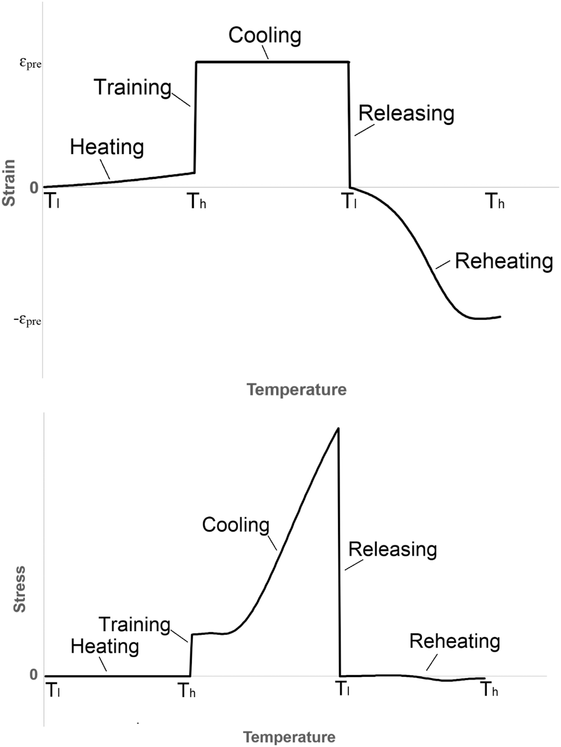

Shape memory polymers have a switchable and reversible molecular structure. As the temperature is lowered from a temperature above the glass transition temperature, T_g, under loading, the molecular structure gradually locks and fixes a temporary shape. When the temperature approaches T_g from a low temperature, the molecular structure reverses to its original state, releasing the strain stored in the material. We define frozen fraction $\left({\varnothing }_f\right)$ as the ratio of the material in a temporary (trained) phase in an elemental volume of the materials to that in its permanent phase. The frozen fraction $\left({\varnothing }_f\right)$ is defined at any temperature (T using a two-parameter $\left(c_f, n\right)$ relationship from Ref. 21 as given in equation (1). The frozen fraction at any material point in the structure determines the strain stored $\left({\varnothing }_f\mathrm{>}0\right)$ ) in the training step.

${\varnothing }_f=1-\frac{1}{1+c_f{\left(T_h-T_{now}\right)}^n}$

(1)

$E_e=3Nk{T}_{now}$

(2)

$\frac{1}{E_m\left({\varnothing }_f\right)}=\frac{{\varnothing }_f}{E_i}+\frac{1-{\varnothing }_f}{E_e}$

(3)

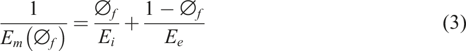
The modulus of the shape memory polymer at any material point is determined by the frozen fraction and the material’s elastic (E_e) and entropic (E_i) moduli. The entropic modulus, E_i, is assumed to be constant in the temperature range considered. E_e is a linear function of temperature due to the rubbery elasticity of a network polymer. ²¹ The modulus of SMP, E_m, as a function of the frozen fraction $\left({\varphi }_f\right)$ of the polymer, is shown in equation (3).

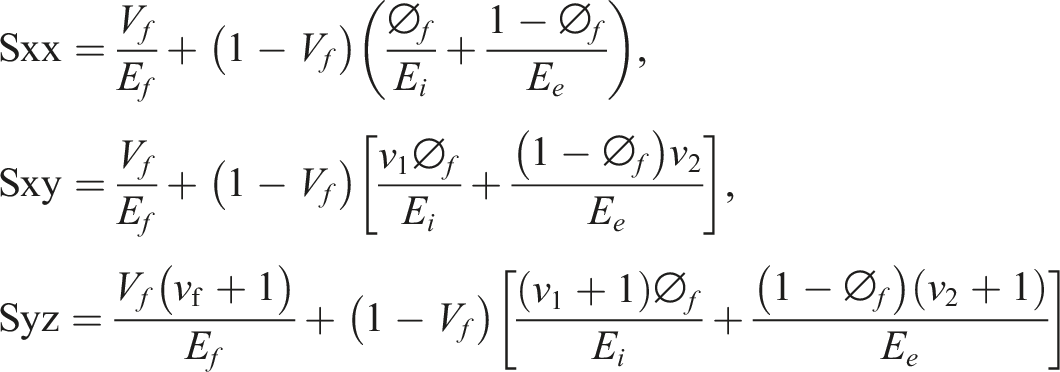
The orthotropic moduli (E₁, E₂ = E₃) of the SMPCs can be obtained by homogenization and the inclusion modulus, E_f. The inclusion is assumed to be linear elastic, and the modulus is temperature independent. The effect of strain storage is limited to the matrix alone. $V_f$ is the reinforcement (inclusion) volume fraction. Since the SMPCs have a glassy state under low temperature and a rubbery state under high temperature, Poisson’s ratio of SMPs is defined as ν₁ for low temperature and ν₂ for high temperature. The Poisson’s ratio of the inclusion is defined as ν_f. With inclusions without shape memory properties, Poisson’s ratio of SMPs changes as the phase-fraction changes, but Poisson’s inclusion ratio is assumed to be constant. If the compliance matrices of inclusion [A _f ] and that of the matrix under low temperature [A _l ] and high temperature [A _h ] are known, the compliance matrix of the random-discontinuous inclusion-loaded SMP matrix composite is assumed as

$\left[\mathbf{A}\right]=\left\{\left[{\mathbf{A}}_{\mathit{h}}\right]\mathit{*}\left(1-{\varnothing }_f\right)+\left[{\mathbf{A}}_{\mathit{l}}\right]\mathit{*}{\varnothing }_f\right\}\ast \left(1-V_f\right)+\left[{\mathbf{A}}_{\mathit{f}}\right]\mathit{*}{V}_f$

(4)

where

$\left[\mathbf{A}\right]=\left[\begin{array}{cccccc}{\text{S}}_{xx}& {\text{S}}_{xy}& {\text{S}}_{xy}& 0& 0& 0\\ {\text{S}}_{xy}& {\text{S}}_{xx}& {\text{S}}_{xy}& 0& 0& 0\\ {\text{S}}_{xy}& {\text{S}}_{xy}& {\text{S}}_{xx}& 0& 0& 0\\ 0& 0& 0& {\text{S}}_{yz}& 0& 0\\ 0& 0& 0& 0& {\text{S}}_{yz}& 0\\ 0& 0& 0& 0& 0& {\text{S}}_{yz}\end{array}\right]$

$\begin{array}{l}\text{Sxx}=\frac{V_f}{E_f}+\left(1-V_f\right)\left(\frac{{\varnothing }_f}{E_i}+\frac{1-{\varnothing }_f}{E_e}\right),\hspace{0.17em}\\ \text{Sxy}=\frac{V_f}{E_f}+\left(1-V_f\right)\left[\frac{v_1{\varnothing }_f}{E_i}+\frac{(1-{\varnothing }_f)v_2}{E_e}\right],\hspace{0.17em}\\ \text{Syz}=\frac{V_f\left(v_{\text{f}}+1\right)}{E_f}+\left(1-V_f\right)\left[\frac{\left(v_1+1\right){\varnothing }_f}{E_i}+\frac{\left(1-{\varnothing }_f\right)\left(v_2+1\right)}{E_e}\right]\end{array}$

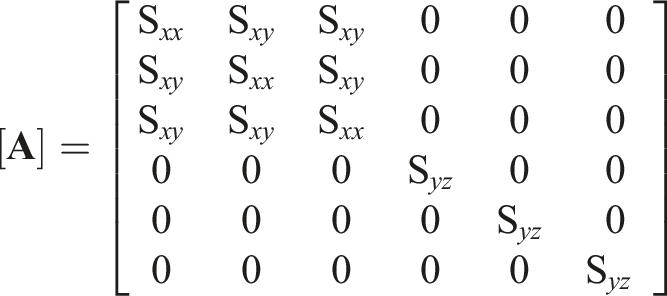
The strain, storage strain, and stress are denoted by

$\left\{\mathit{\epsilon }\right\}={\left\{{\epsilon }_x{\epsilon }_y{\epsilon }_z{\epsilon }_{yz}{\epsilon }_{xz}{\epsilon }_{xy}\right\}}^T$

(5)

$\left\{{\mathit{\epsilon }}_{\mathit{S}}\right\}={\left\{{\epsilon }_{Sx}{\epsilon }_{Sy}{\epsilon }_{Sz}{\epsilon }_{Syz}{\epsilon }_{Sxz}{\epsilon }_{Sxy}\right\}}^T$

(6)

$\left\{\mathit{\sigma }\right\}={\left\{{\sigma }_x{\sigma }_y{\sigma }_z{\sigma }_{yz}{\sigma }_{xz}{\sigma }_{xy}\right\}}^T$

(7)

$\left\{\mathit{\alpha }\right\}={\left\{\begin{array}{cccccc}{\alpha }_x& {\alpha }_y& {\alpha }_z& 0& 0& 0\end{array}\right\}}^{\text{T}}$

(8)

where ${\epsilon }_x=du/dx$ , ${\epsilon }_y=dv/dy$ , ${\epsilon }_z=dw/dz$ , ${\epsilon }_{yz}=\left(dw/dy+dv/dz\right)$ , ${\epsilon }_{xz}=\left(dw/dx+du/dz\right)$ , and $\hspace{0.17em}{\epsilon }_{xy}=\left(dv/dx+du/dy\right)$

The frozen fraction dependent constitutive relation for the SMPC can be written as follows

$\left[\mathit{\sigma }\right]=\left[\mathbf{C}\right]\left(\left\{{\mathit{\epsilon }}_{\mathit{total}}\right\}-\left\{{\mathit{\epsilon }}_{\mathit{S}}\right\}-\left\{\mathit{\alpha }\right\}\mathrm{\Delta }T\right)$

(9)

where

$\left[\mathbf{C}\right]={\left[\mathbf{A}\right]}^{-1}$

For 3D deformation motion, the storage strain $\left({\epsilon }_S\right)$ is developed from 1D to 3D as

$\frac{\text{d}\left\{{\mathit{\epsilon }}_{\mathit{S}}\right\}}{\text{d}T}=\left[{\mathbf{S}}_{\mathbf{h}}\right]\left[\mathbf{C}\right]\left(\left\{\mathit{\epsilon }\right\}-\left\{{\mathit{\epsilon }}_{\mathit{S}}\right\}-\left\{\mathit{\alpha }\right\}\mathrm{\Delta }T\right)\left(\frac{\text{d}{\varnothing }_f}{\text{d}T}\right)$

(10)

${\left\{{\mathit{\epsilon }}_{\mathit{s}}\right\}}_{\mathit{i}+1}={\left\{{\mathit{\epsilon }}_{\mathit{s}}\right\}}_i-{\left\{\mathrm{\Delta }{\mathit{\epsilon }}_{\mathit{S}}\right\}}_i$

(11)

where $\left[{\mathbf{S}}_{\mathbf{h}}\right]$ is the compliance related to E_e of the SMPC, ${\left\{{\mathit{\epsilon }}_{\mathit{s}}\right\}}_i$ are the storage strains at current temperature step and the previous temperature step during the heating and cooling process, respectively. Equations (10) and (11) are solved and $\left\{{\mathit{\epsilon }}_{\mathit{S}}\right\}$ is computed incrementally for each ΔT.

The constitutive relationship in equations (4)–(11) was implemented in a 3D finite element analysis. The displacement field satisfying the force-equilibrium at any temperature is obtained using the principle of virtual displacements

${\displaystyle {\int }_{\text{V}}{\overline{\mathrm{ϵ}}}^T\mathit{\sigma }}\hspace{0.17em}\text{d}V={\displaystyle {\int }_V{\overline{U}}^T{\mathbf{f}}^B}\hspace{0.17em}\text{d}V+{\displaystyle {\int }_{\text{S}}{\overline{U}}^{S^{\mathit{T}}}{\mathbf{f}}^S}\hspace{0.17em}\text{d}S+{\displaystyle \sum _i{\overline{U}}^{i^{\mathit{T}}}{\mathbf{F}}^i}$

(12)

where the external work done the body forces, surface tractions, and concentrated forces ( ${\mathbf{f}}^B$ , ${\mathbf{f}}^S$ , and ${\mathbf{F}}^i$ , respectively) going through the virtual displacement $\overline{\mathrm{U}}$ are given on the right side of equation (12). All virtual quantities are signified with an overbar. The superscript S denotes boundaries on which traction is applied and the superscript i denotes the displacements at the point where the concentrated forces ${\mathbf{F}}^i$ are applied. Substituting the constitutive relationships into the internal energy integral results in equation (13).

${\displaystyle {\int }_V{\overline{\mathrm{ϵ}}}^T\mathit{\sigma }}\hspace{0.17em}\text{d}V={\displaystyle {\int }_V\left[\mathbf{C}\left({\varphi }_{\text{f}}\right)\right]\left(\left\{\mathit{\epsilon }\right\}-\left\{{\mathit{\epsilon }}_{\mathit{S}}\right\}-\left\{\mathit{\alpha }\right\}\mathrm{\Delta }T\right):\left\{\overline{\mathit{\epsilon }}\right\}}\hspace{0.17em}\text{dV}$

(13)

Equations (12) and (13) are solved over 3D domains using FEM and an incremental temperature stepping scheme. Simulations are performed following the previously described five-step training and recovery process. Temperature is increased from T_l to T_h in the first step. The material softens, and any thermally induced stress and deformation fields are set up. The training step entails applying all external deformations or loads. The temperature is lowered from T_h to T_l while keeping the external load/deformation constraints in place. The load and deformation constraints are removed in the fourth or the release step. This completes the training of the structure to a temporary shape. The fifth step simulates the shape recovery. In this step, the temperature is raised from T_l to T_h, and the deformation of the structure is observed as the shape transition takes place. In all steps, we observe the mechanical stress, strain, storage strain states within the structure. Material parameters for SMP and SMPC structures are presented in Table 2. Reference SMP material ³⁶ is applied for verification of the published model. Poisson’s ratio is set as 0.28 for the glassy state and 0.49 for the rubbery state. The volume fraction of inclusion is set as zero for simulations of un-reinforced SMPs. FreeFem++, ⁵¹ a free finite element package, was used to implement the present constitutive model and perform shape recovery simulations.

Results: shape recovery in 3D SMP structures

We simulated the shape recovery after tension, compression, bending, torsion, and in a plate with a hole using the developed temperature-dependent constitutive relationship within finite element analysis. Several mesh densities were used to study the effect of mesh refinement on the solutions. The simulations were carried out following the five-step training and recovery procedure described earlier and by changing the temperature of the system in 1 K step increments. The stress, strain and storage strain tensors were computed over the entire structure, and temperature-dependent changes to the stress and strain states are tracked at a selected node on the structure. The first two cases (tension and compression) also serve as the verification problem for our implementation, as we can compare the results to those published in Ref. 36. The SMP material used in the published work was an epoxy-based thermoset EMC resin named CTD–DP5.1. ³⁶

With the temperature-dependent Poisson’s ratio, the stiffness matrix evolution is plotted as Figure 2. The C₁₁ and C₃₃ gradually drop as the temperature increases in the heating and reheating steps, then raise back in the cooling step. Due to the variation of Poisson’s ratio, C₁₂ changes proportionally as the temperature starts increasing or decreasing at the beginning of the heating, cooling, and reheating steps. However, it also follows the same trend as C₁₁ and C₃₃ when the temperature reaches the T_g.

Figure 2.

Compliance matrix variations during the heating, training, cooling, and recovery (reheating) steps.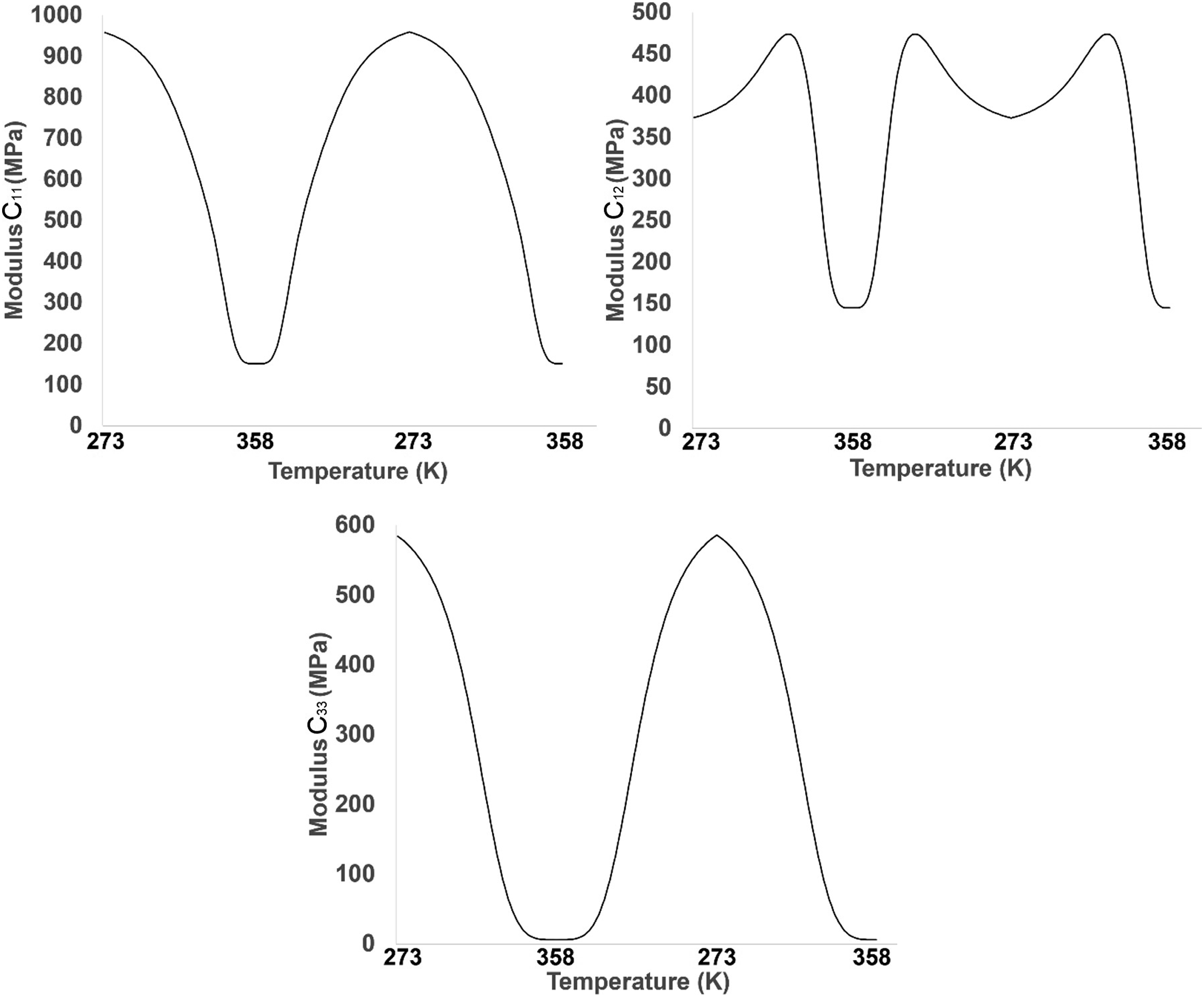

As the first case, we studied the shape recovery of a dog bone sample that is loaded in tension. Figure 3 shows the three indicators that were tracked in this study. First, we observed the evolution of a significant strain component (e_y) through the five steps. This figure shows the results at the end of each simulation step. The label “Heat” indicates heating to the high temperature (T_h), the “Train” label indicates the application of the training strains at T_h, cooling to T_l under the training restraints on the structure is labeled “Cool,” the release of the training restraints on the structure at T_l is indicated by “Release” and reheating to observer the shape recovery behavior is indicated by “Recover.” The analysis is conducted with an original coordinate system reference at the low-temperature T_l, and strains and stresses after the heating, training, cooling, and releasing steps are computed with respect to that coordinate system. At the end of the “Release” step, the mesh is updated to freeze the deformations, and the stresses and strains computed in the “Recover” step take the deformed structure as the reference geometry. The top row in Figure 3 shows the evolution of the strain component (e_y) and shows a training strain of 0.1 applied in the “Train” step. The middle row shows the strain storage (e^s_y) within the sample. The figure shows train concentrations at the corners where the sample transitions from the gage cross-section to the grip cross-section. The bottom row shows the evolution of the stress component (σ^s_y) at the end of the five simulation steps.

Figure 3.

Top row: Extensional strain (ɛ_y); Middle row: storage strain (ɛ^s_y); Bottom row: stress (σ_y) development in the dog bone sample.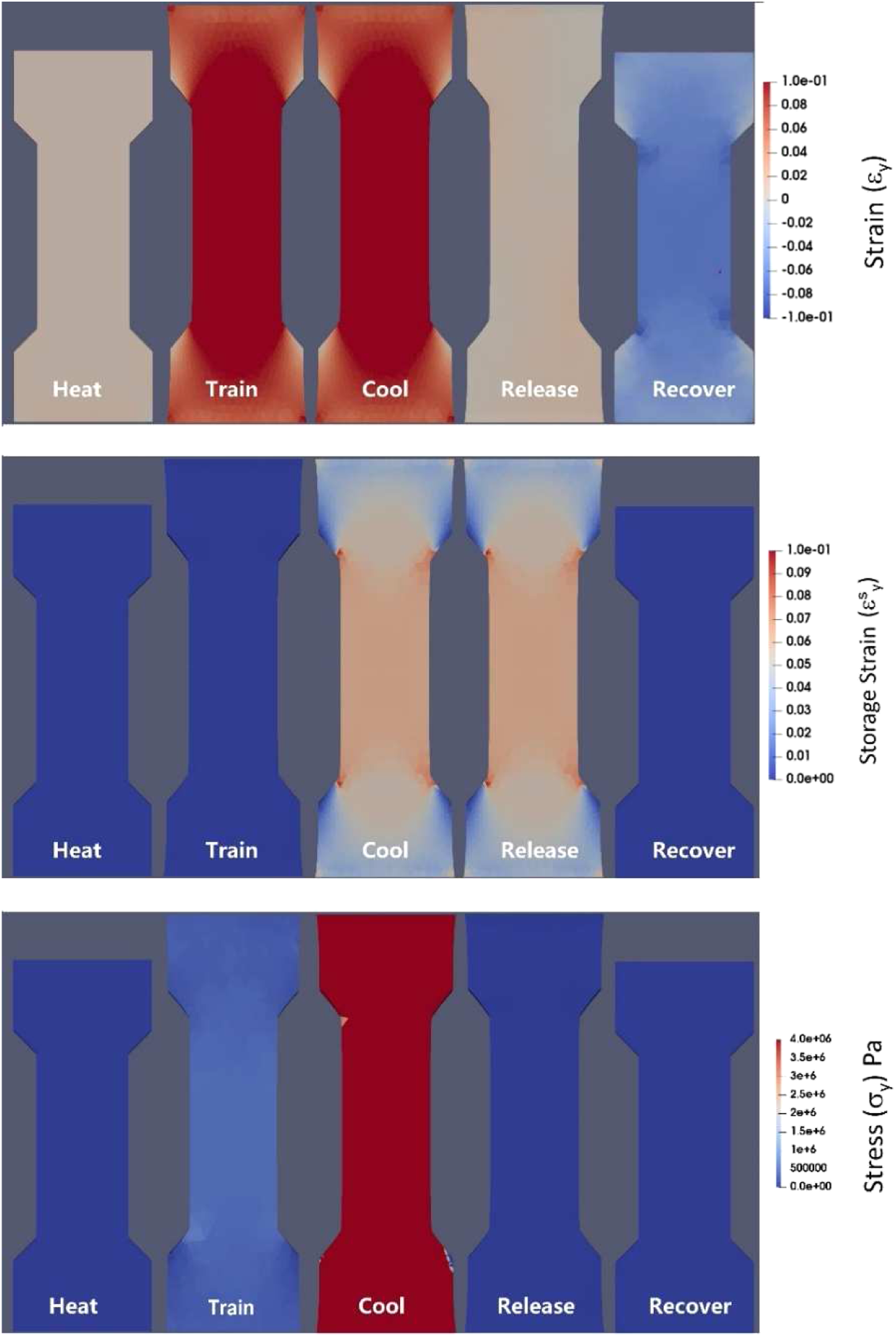

Figure 4 shows the evolution of the strain and stress components at one location in the structure. We selected a nodal point at the center of one surface of the sample to plot the strain and stress data. Figure 4(a) plots the extensional strain (e_y) at the selected point as a function of the temperature. While the training and sample release take place isothermally, the temperature changes during the cooling and reheating steps are shown along the x-axis. Temperature in this and subsequent plots changes on the x-axis from T_h to T_l (“Cool”) step and back from T_l to T_h in the “Recover” step. Figure 4(b) and (c) show the storage strain and stress at the selected point, respectively. The plot also shows the results for several mesh densities. Table 1 shows three mesh sizes (TA, TB, and TC) used for conducting the simulations. The table lists the number of nodes, elements, and maximum element length (L_s) in millimeters. Figure 4(a)–(c) shows that the results are convergent for the smaller mesh sizes. By setting the same pre-strain, the stress response has successfully verified the results published in Ref. 36.

Figure 4.

Strain (a), storage strain (b), and stress (c) responses at a selected point in the gage section during the heating, training, cooling, and recovery (reheating) steps.

Table 1.

FEM meshes used in the computation (L_s is the shortest element length).

Label	Nodes, elements, Ls (mm)	Label	Nodes, elements, Ls (mm)	Label	Nodes, elements, Ls (mm)	Label	Nodes, elements, Ls (mm)
TA	5302, 29368, 1.41	CA	16151, 95520, 7.5	WA	26571, 157920, 60	HA	10208, 56056, 0.393
TB	17696, 100844, 0.94	CB	52486, 312120, 4	WB	78671, 469920, 20	HB	15070, 82424, 0.196
TC	38703, 223172, 0.71	CC	119621, 713120, 3	WC	141191, 844320, 11.11	HC	24156, 131448, 0.098
BA	26901, 155200, 0.5
BB	87451, 511200, 0.33
BC	203401, 1196800, 0.25

FEM: finite element method.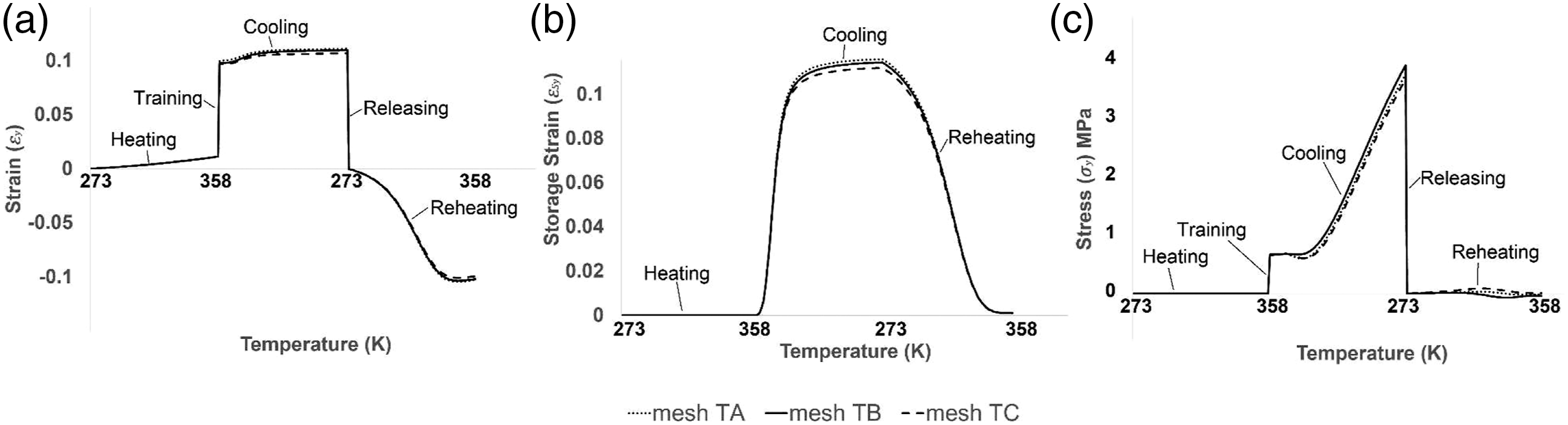

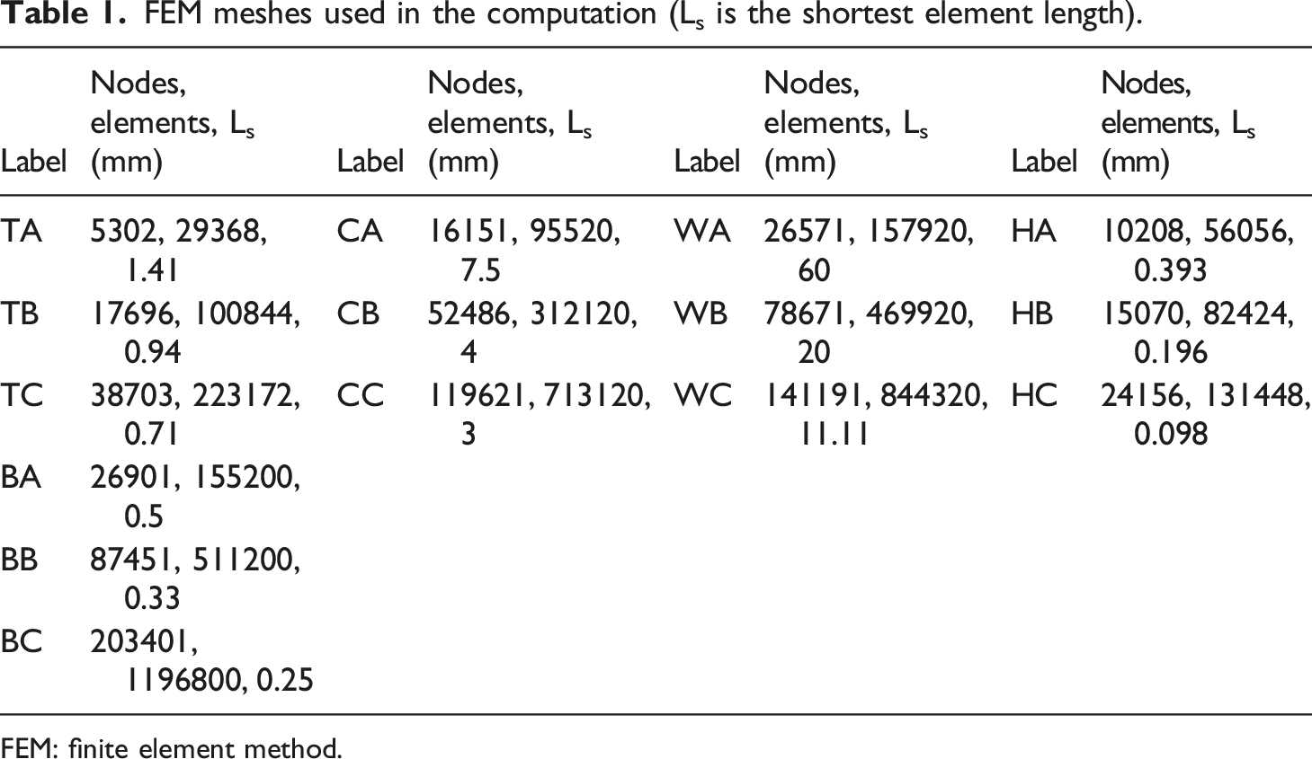
Figure 5 shows the application of compressive training strain, storage strain, and stress profile at a selected point at the center of the structure. This plot also shows the profiles for three different mesh sizes (CA-CC), as listed in Table 1. Figure 5(a) shows the application of a total compressive training strain (ε_y) of 0.1. After the heating step, the sample elongates due to thermal expansion. The training strain brings the structure into compression. Figure 5(b) and (c) show the storage strain and stress profiles through the training and shape recovery process. The stress response matched the reference results in Ref. 36.

Figure 5.

Recovery with compression.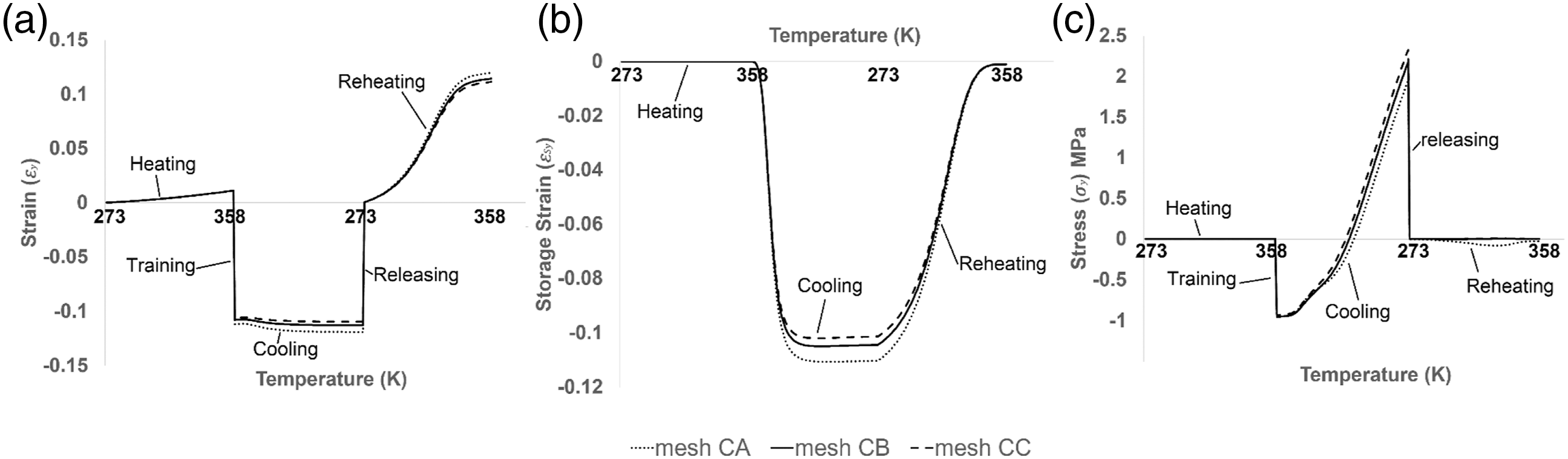

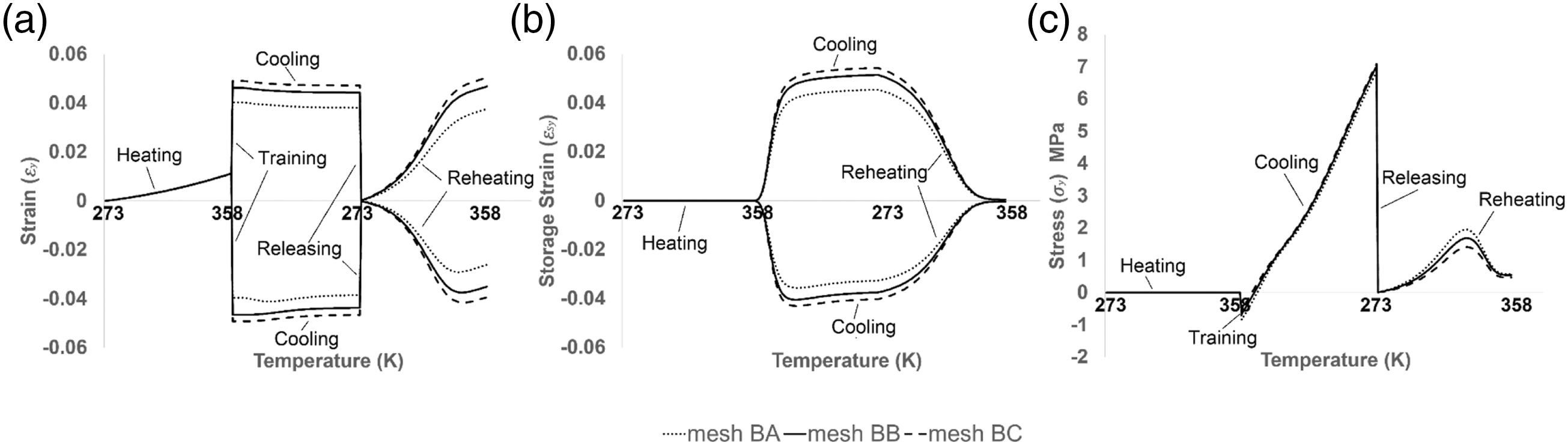
Figure 6 shows the shape recovery after training under bending loading. An external force was applied to one side surface of the sample. The simulation shown in this figure depicts the recovery of an SMP polymer section that after training under bending loads. The structure stores a complex 3D strain state in this case, and the extensional strain distributions (ε_y) are shown in Figure 6. Two points on this structure were identified on the surface at the center of this structure. The strain, storage strain, and stress distributions are plotted in Figure 7 with three different mesh densities (BA-BC). The strain (tension and compression side), storage strain (tension and compression), and the stress (compression side only) are shown at selected nodal points at the center cross-section of the sample. The computations were made for several mesh densities, BA-BC, as outlined in Table 1.

Figure 6.

Shape recovery after bending.

Figure 7.

Strain, storage strain, and stress response of two selected points on the bent sample.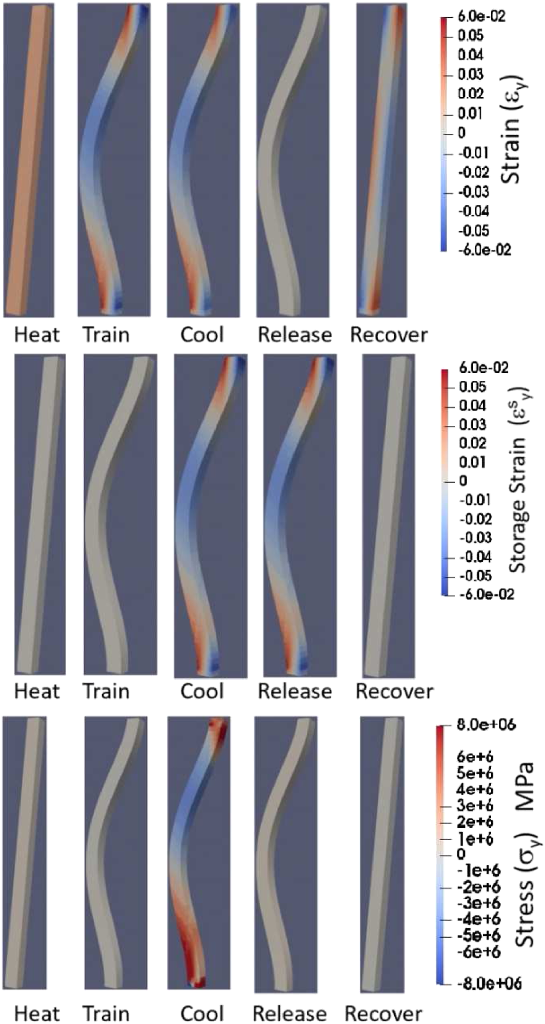

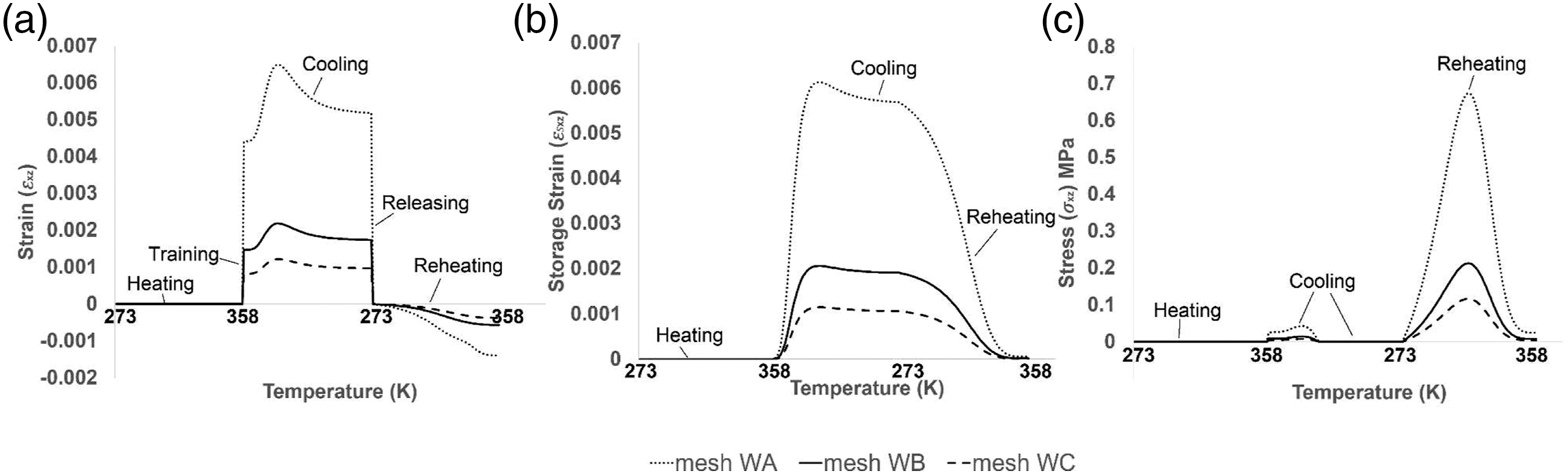
For the twisting motion, the sample is fixed on the bottom side and twisted on the top side, as shown in Figure 8. The shape recovery response when the sample is twisted 60° about the y-axis is shown in Figure 9. In this case, the shear strain (ε_xz) was observed and plotted. The storage and release of the shear strain in the structure are demonstrated in this case. Significant mesh dependence is shown in the results, but the results are seen to converge with decreasing element sizes. The most refined mesh (WC) that we used had 141,191 nodes (423,573 degrees of freedom). Based on equation (9), shear stress reduces to zero after the shear strain has been fully stored ({ɛ _total } = { ɛ _S }) in the cooling step since there is no thermal stress.

Figure 8.

Torsional loading setup.

Figure 9.

Torsional loading.

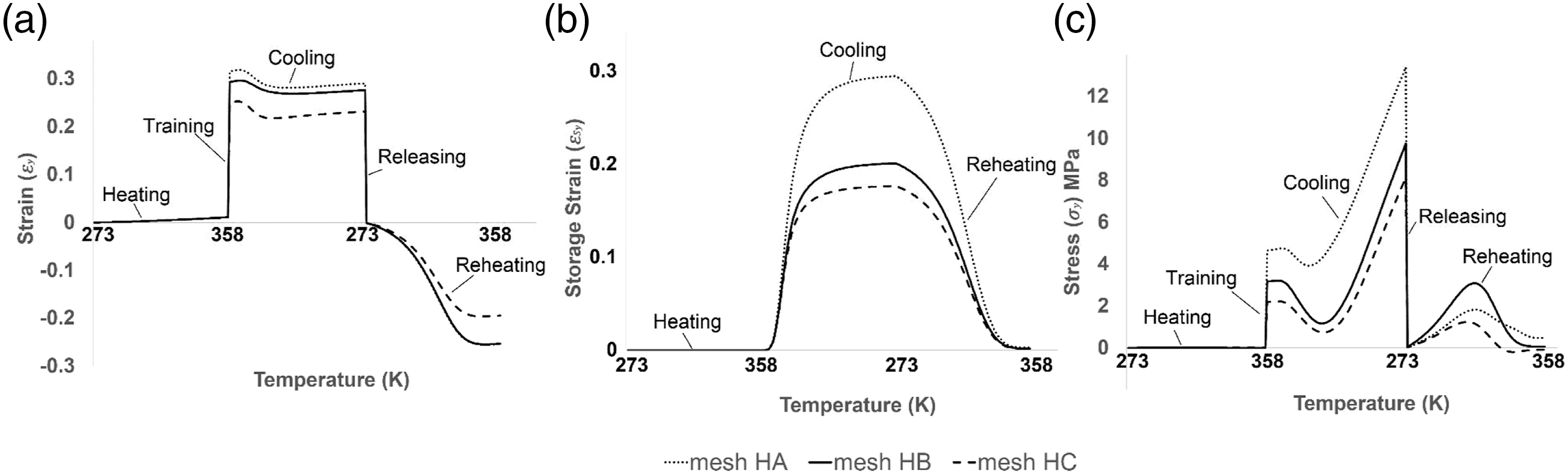
The storage of a multi-axial state of stress was examined with a dog bone–shaped structure with an open hole. The shape recovery response was checked in the presence of holes, which leads to stress concentration. As a kind of structure defect, the effect of stress concentration on the strain, storage strain, and stress has been investigated. Figure 10 shows a strain component (Top row), a storage strain component (Middle row), and a stress component (Bottom row) at the end of the five simulation steps. Figure 11 shows the stress, strain, and storage strain at the point near the hole in the region where there is a high-stress concentration. For different mesh densities (HA-HC), we kept reducing element sizes around holes but kept the same element size for the rest of the sample.

Figure 10.

Top row: strain; middle row: storage strain; bottom row: stress.

Figure 11.

Strain response of the tensioned dog bone sample with a hole.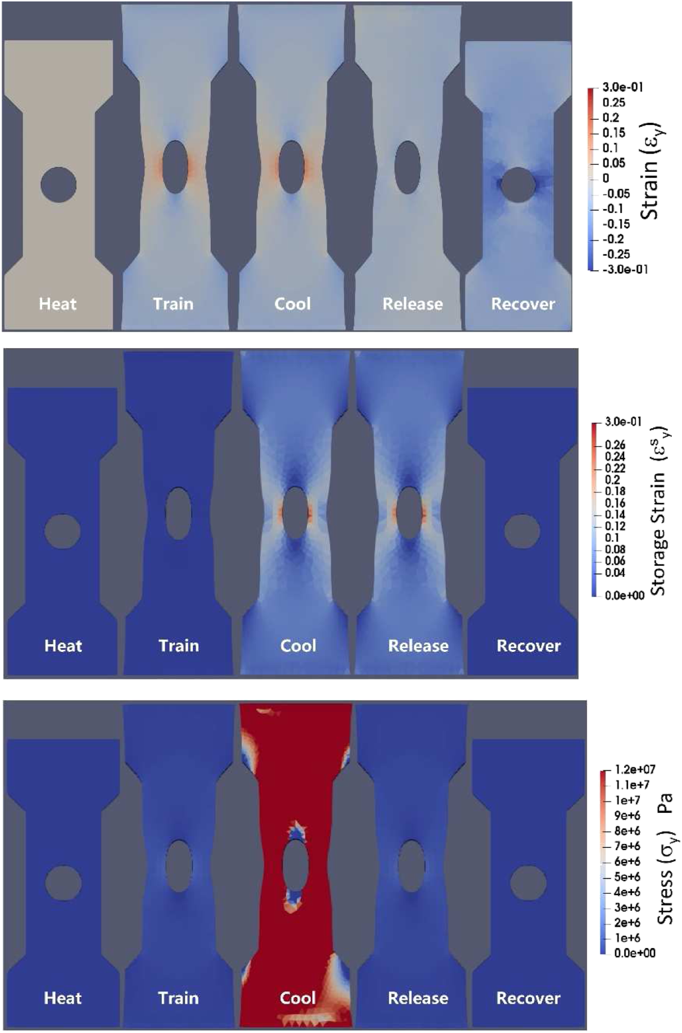

The five cases reported in this section serve as verification examples for the developed constitutive model and its implementation into the 3D FEM.

Results: shape recovery in SMPC

In this section, we describe the validation of the model to predict the shape recovery in a carbon black–reinforced PLA structure produced by the Fused Filament Fabrication AM method. In this effort, we applied the model to additively manufactured SMPC samples produced from carbon black–loaded thermoplastic PLA filaments (commercially available as Proto-Pasta ⁵² conductive filament). The filament is a compound of Natureworks 4043D PLA, a dispersant and conductive carbon black. It is reported to have a filament electrical volume resistivity of 15 Ω-cm for the molded resin, and 30 Ω-cm perpendicular to the layers and a through the layer volume resistivity of 115 Ω-cm. The SMPC samples were printed on a QIDI X-pro 3D printer (Qidi Technology, Inc., Zhejiang, China). The model requires two moduli, E_e and E_i, and two parameters (c _f , n) that determine the relationship between frozen fraction and temperature for the SMPC material. We used a dog bone sample, designed as shown in Figure 12, to determine the required properties.

Figure 12.

Design of the sample used for 3D printing and experiments. (All dimensions are in mm).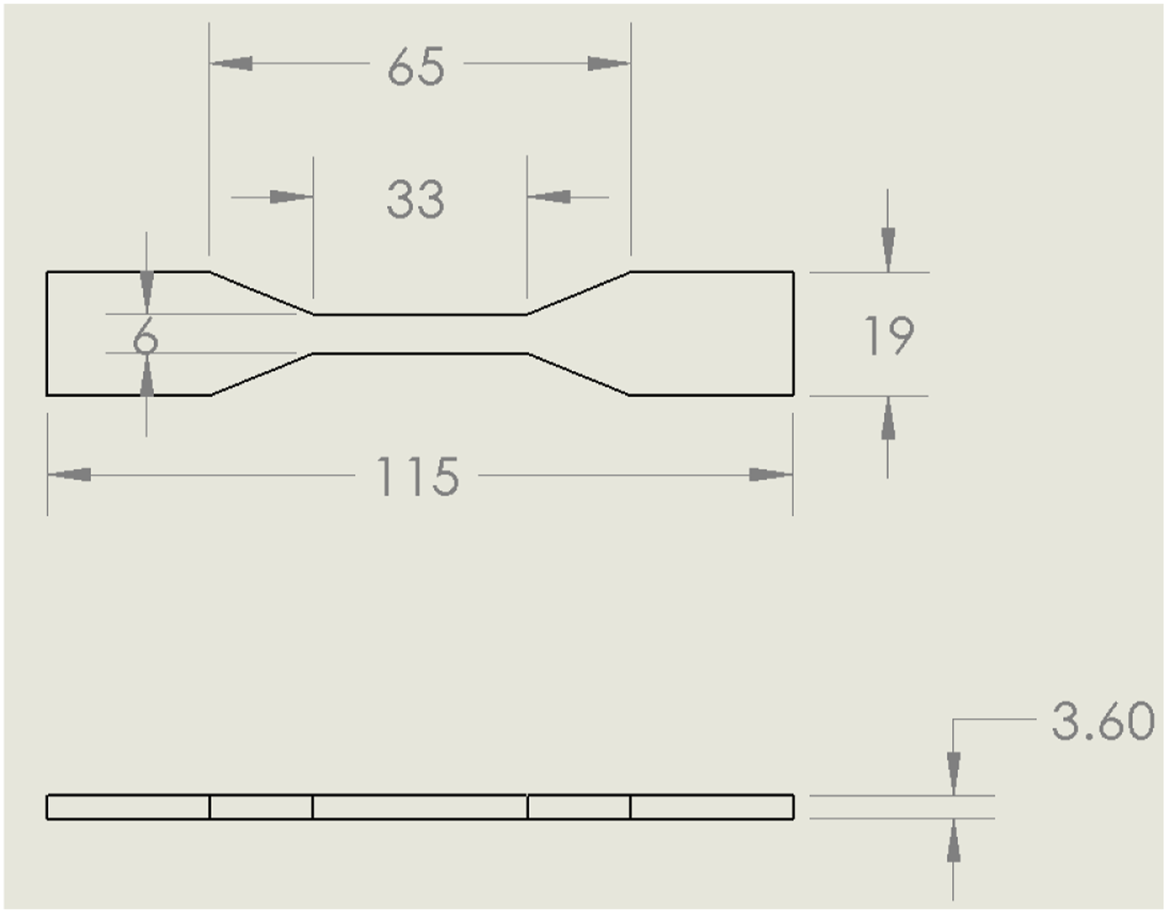

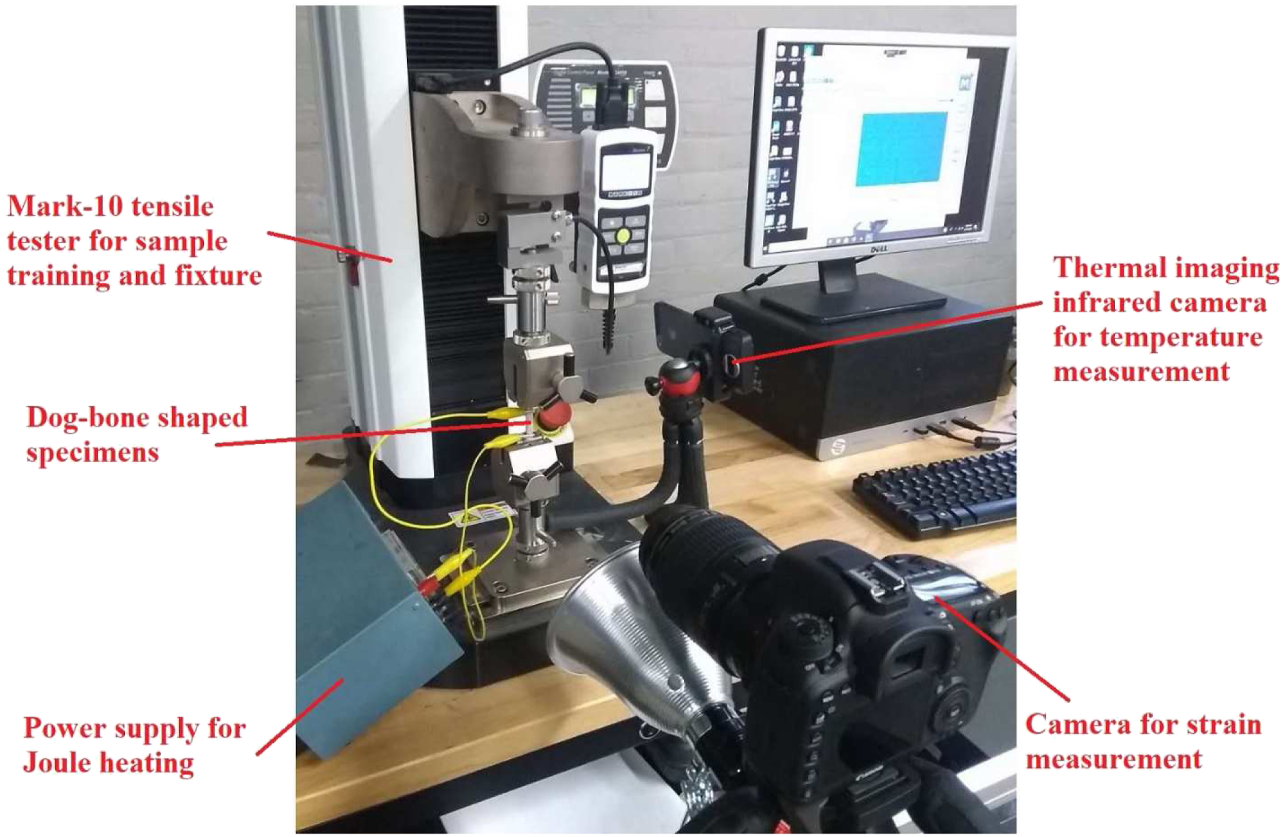
In order to characterize the parameters that determine the frozen fraction, ${\varnothing }_f$ , we conducted uniaxial strain storage and recovery experiments. ³⁶ The sample was trained with an applied uniaxial strain, and strain recovery during reheating was monitored using Digital Image Correlation (DIC) technique. The experimental setup is shown in Figure 13, which consists of a tensile testing machine along with a camera for obtaining images for the DIC and a thermal camera observing the temperature states. Since the sample had a moderate amount of electrical conductivity due to the presence of conductive inclusion, Joule heating could be used to heat the sample uniformly. The internal heating eliminates the delay in activating the shape recovery associated with the thermal diffusion. ⁵³ The strain $\left({\mathit{ϵ}}^{\ast }\left(T\right)\right)$ measured during the reheat/recovery step reflects the storage strain level. The frozen fraction is estimated as the fraction, $\left({\mathit{ϵ}}^{\ast }\left(T\right)\right)/{\mathit{ϵ}}_{pre}$ .

${\varnothing }_f\left(T\right)=\frac{{\mathit{ϵ}}^{\ast }\left(T\right)}{{\epsilon }_{pre}}=1-\frac{1}{1+c_f{\left(T_h-T_{now}\right)}^n}$

(14)

Figure 13.

The experimental setup used for heating, loading and strain measurement.

The parameters c_f and n are obtained by fitting (equation (1)) to the experimentally observed, ${\epsilon }^{\ast }/{\epsilon }_{pre}$ curve. Since the sample was conductive, it could be heated by Joule heating. The temperature of the sample is measured using a thermal imaging infrared camera. The strain of the sample is measured by using a high-speed camera with DIC technology. A speckle pattern was created with spray paint, as shown in Figure 14. Copper tape is used as contact pads for Joule heating. A constant cooling/heating rate in the temperature range between T_l and T_h is needed to acquire equilibrium in these samples.

Figure 14.

The dog bone sample prepared with a speckle pattern and copper tabs for Joule heating.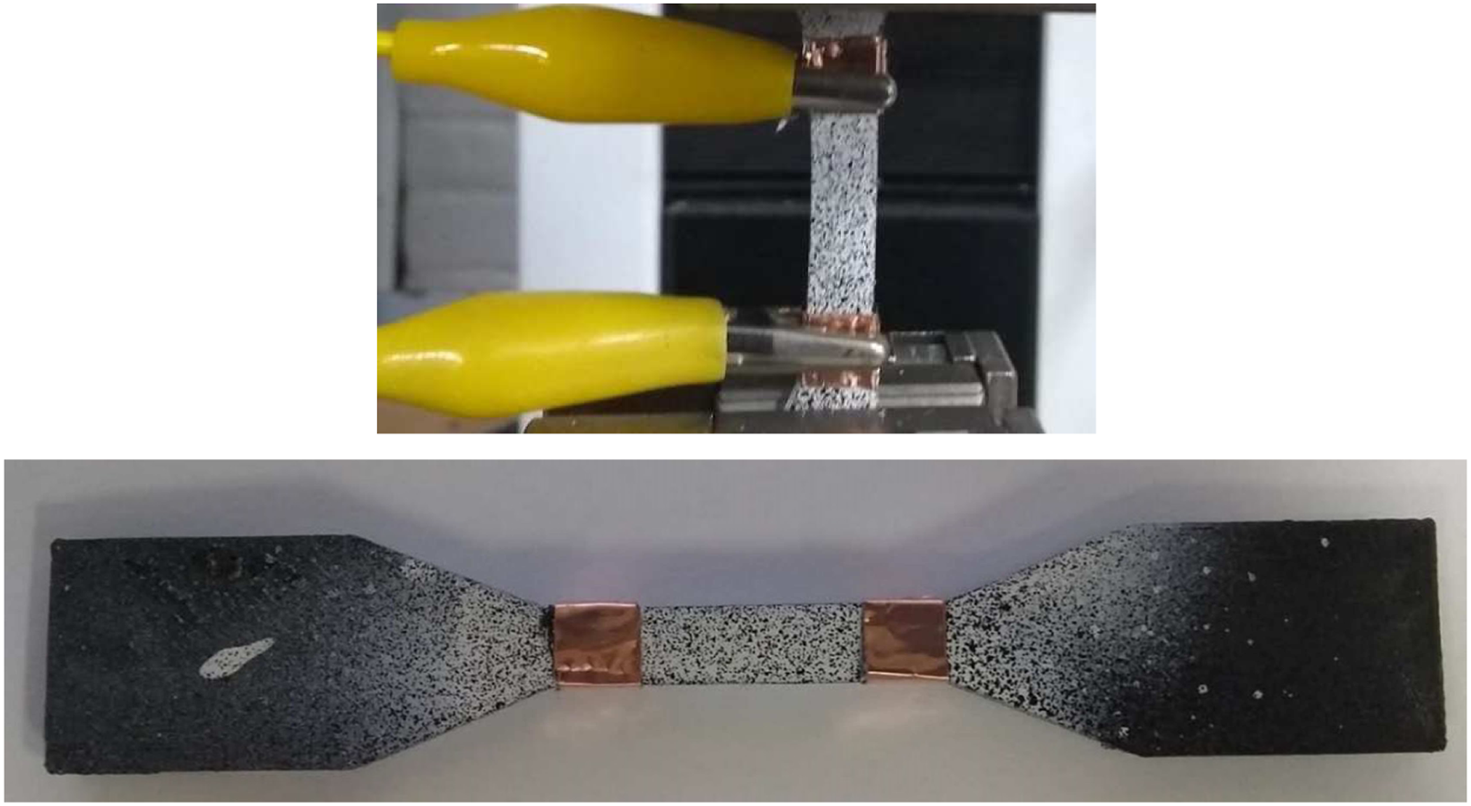

The samples were tested using the procedure given below:

1. Grip the samples with no load is applied.

2. Heat the samples until T_h, (>T_g).

3. In the softened state, load the sample (in tension).

4. Cool the samples to T_l and release the grips after the sample reach T_l.

5. Reheat the sample to T_h and measure the strain.

Figure 15 shows the strain recovery during the reheating step. The shape recovery in the samples tested initiates at a transition temperature of 323 K. The sample was then fixed between the grips, and recovery force was measured as the temperature was raised past 323 K. The force sensor detects recovery force at 323 K and the three tested samples as produced. A maximum recovery force was observed to be 6.7 N.

Figure 15.

Comparison of simulation and experimental results for parts 3D printed with composite filaments.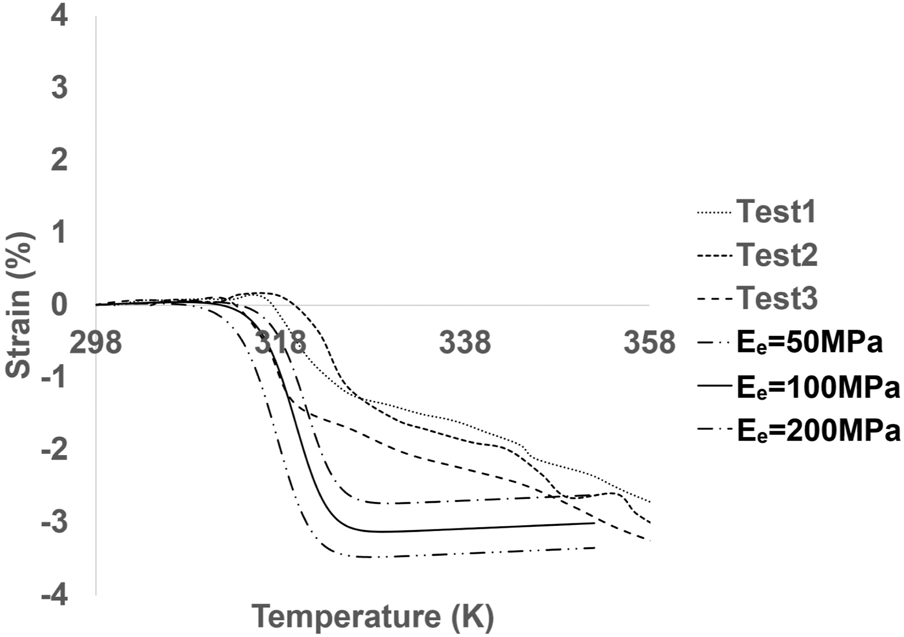

Based on the experimental result of the conductive composites-based samples and equation (1), two variables of the function ϕ_f(T), c_f, and n can be determined by fitting the strain ratio data into Figure 16. ${\mathit{ϵ}}^{\ast }\left(T\right)$ can be calculated by subtracting the recovered strain ${\epsilon }_y$ from training strain ${\mathit{ϵ}}_{pre}$ . ${\mathit{ϵ}}^{\ast }\left(T\right)$ divided by the training strain ${\mathit{ϵ}}_{pre}$ can be applied to fit with the frozen fraction curve.

Figure 16.

Curve fitting of the stored strain divided by the pre-deformation strain for calculating two variables of the function ϕ_f(T), c_f, and n.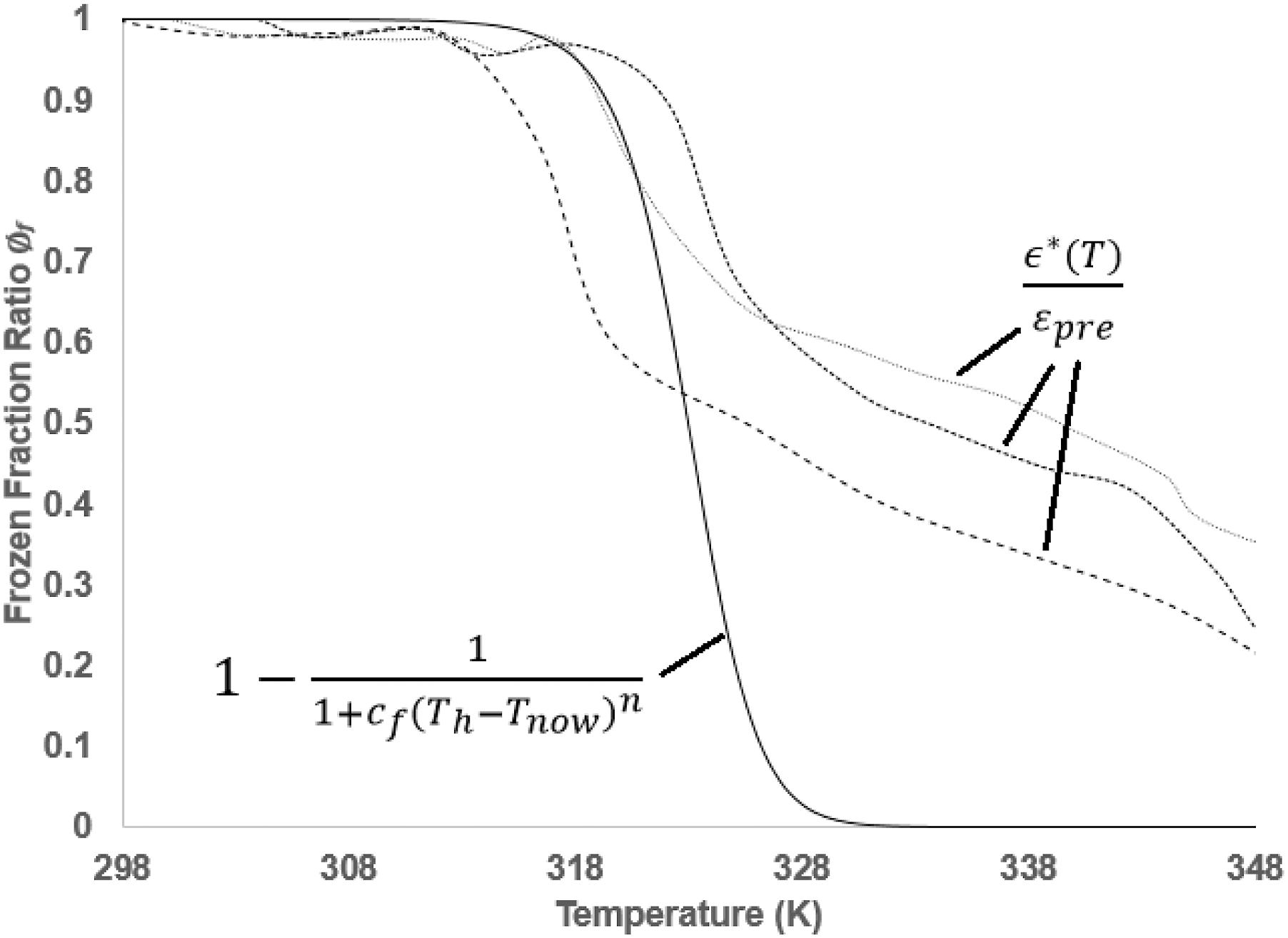

The value of Young’s modulus at low temperature has been measured, so E_i can be obtained from equation (3). Due to the reinforcement, E_e is estimated as a range of 50–200 MPa. The shape recovery of the dog bone sample used in the experiment is simulated using values of the parameters shown in Table 2. A correlation of the experimental and simulation results is shown in Figures 17 and 18. Figure 15 shows the comparison of simulation and experimental results. Three values of E_e are set for simulation to generate the strain response. The experimentation shows a strong correlation to the performance predicted by the constitutive model.

Table 2.

Material constants for the two materials analyzed in this effort.

	Thermoset used for model validation (SMPs) 36	Conductive thermoplastic AM material for model calibration and validation (SMPCs)
n	4	17
Cf (1/K4)	2.76×10−5	2.12×10−25
Ee (MPa)	8.8	50–200
Ei (MPa)	750	1500
Ef (MPa)	N/A	100,000
N (mol/cm3)	5.937×1020	3.421×1027
α (K−1)	−3.16×10−4+1.42×10−6*T	0.55×10−4
Th (K)	358	353
Tl (K)	273	298
ν1	0.28	0.28
ν2	0.49	0.49
νf	0.3	0.3
Vf (%)	0	25

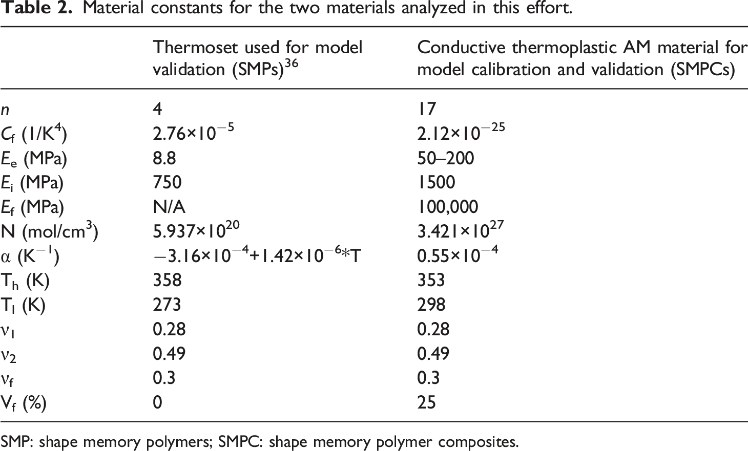
SMP: shape memory polymers; SMPC: shape memory polymer composites.

Figure 17.

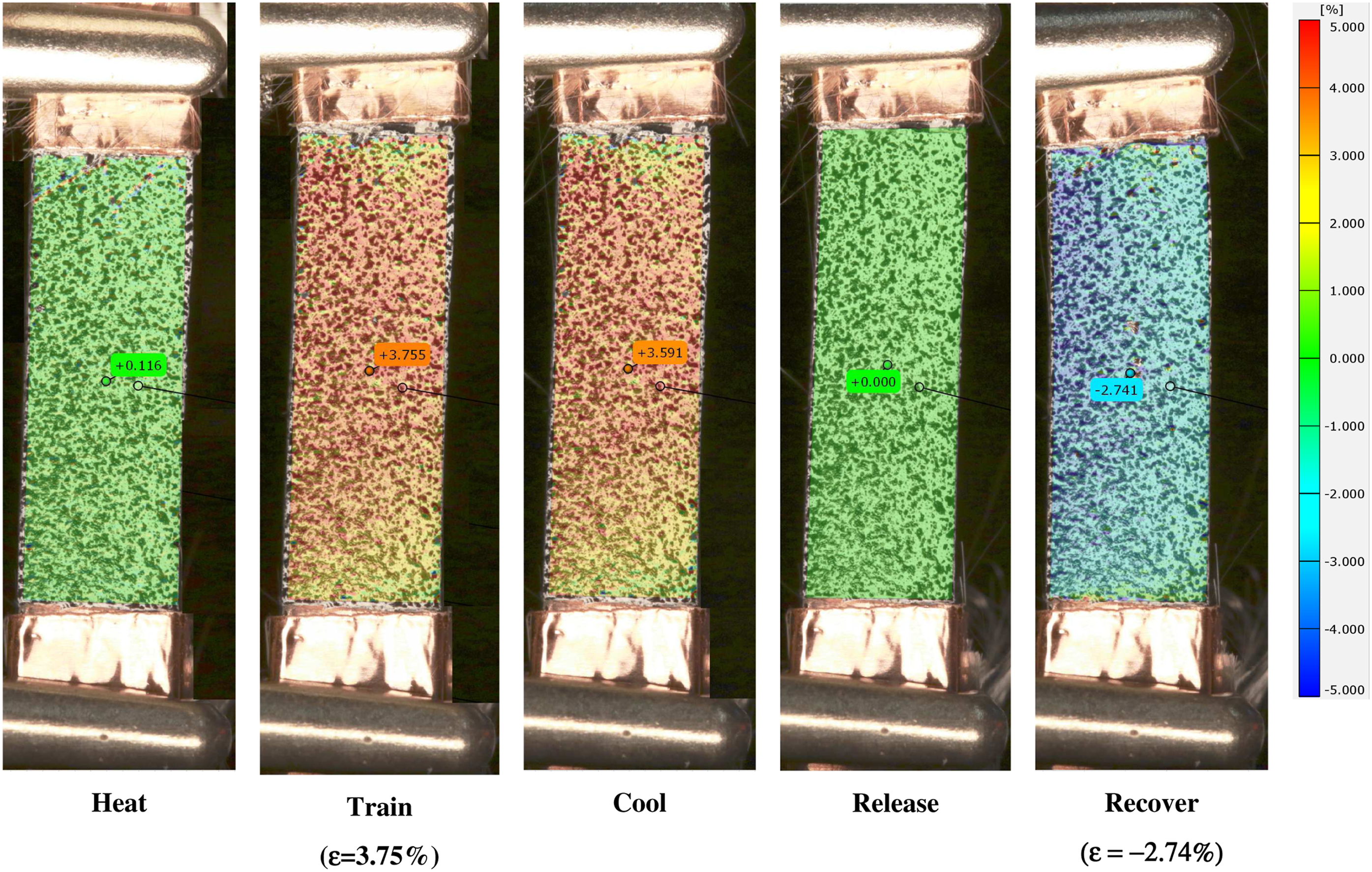
Strain measurements using Digital Image Correlation.

Figure 18.

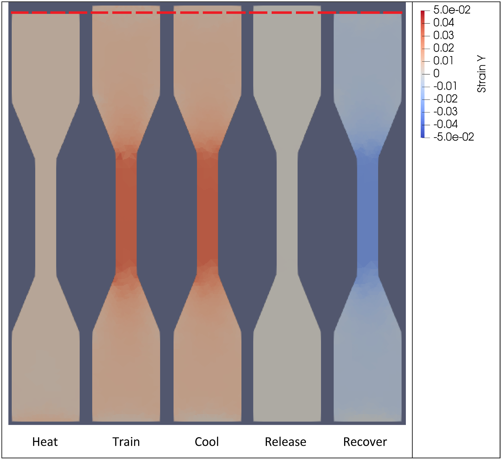
Strain distribution of the tensioned dog bone sample.

Concluding remarks

In summary, a constitutive model to predict the shape recovery after training the temporary shapes with multi-axial thermo-mechanical loadings (tension, compression, bending, and twisting) has been developed. The total strain, storage strain, and stress responses of SMPs during the thermal cycling (heating, training, cooling, releasing, and reheating) have been simulated and analyzed with the consideration of Poisson’s ratio effect. Then, a new SMPC material including stiff inclusion or reinforcement (the inclusion is assumed to have no shape memory properties) is simulated. Model parameters for a new material system were obtained by calibrating the temperature-frozen fraction relationship using a tensile training strain field. The sample was heated using Joule heating, and strain recovery was measured with DIC. Our model uses the frozen fraction field (equation (10)) to determine the storage strain fraction for all strain components (ɛ_xx ɛ_yy ɛ_zz ɛ_xy ɛ_xz ɛ_yz). This implies that all the strain components are stored and recovered at the same rate as determined by $\text{d}{\varnothing }_f/\text{d}T$ . It also leads to the same variation of stiffness in all six stress/strain components. Since the developed constitutive model extends a polymer shape memory response model to include inclusions and into 3D finite element analysis, structural response can be predicted in a generalized way.