Analysis of the partially closed interface crack in orthotropic materials

Abstract

The determination of fracture parameters such as mode I and II stress intensity factors, K_I and K_II , is of considerable practical importance in the analysis and failure prediction of various types of structures. For example, interfacial cracks may develop and propagate in bonded joints or lead to delaminations in composite materials. The finite element method is a powerful technique for analyzing complex structures; however, the singular behavior near crack tips is poorly approximated by conventional finite elements and convergence theorems cease to be applicable at those locations. In a previous paper, a combined analytical and numerical model based on frictionless crack face contact was used to obtain fracture parameters at interfacial cracks in composite laminates in cylindrical bending and subject to transverse loads. In this article, we further consider the method and extend the previous results by considering a variety of shear and normal loads on a cracked bimaterial plate with isotropic or orthotropic materials. Furthermore, additional validation of the method is provided by comparing the results with closed form solutions in the literature for the special case of isotropic materials in a combined tensile and shear field, and good agreement is found. Overall, we conclude that the method provides a practical way to analyze a variety of engineering structures with interfacial cracks.

Introduction

The analysis of cracks at interfaces between orthotropic materials is of significant importance in the study of crack initiation and propagation, especially in composite materials and bonded joints. The solution of the interface crack problem assuming that the crack faces are traction free leads to characteristic oscillatory stresses and displacements near the crack tip. This oscillatory behavior may result in overlapping of crack faces and materials, a physical contradiction. The alternative model proposed by Comninou ¹ provides a more realistic approximation by allowing the possibility of frictionless contact along the crack faces, thus eliminating the overlapping of crack faces. However, a practical and efficient method to determine the stress intensity factors for interface crack problems having a contact region and complex geometries and boundary conditions becomes necessary to solve real-world engineering problems. In a previous paper, a combined analytical and numerical model based on frictionless contact was used to obtain fracture parameters at interfacial cracks in composite laminates in cylindrical bending and subject to transverse loads. ² In the present article, the method is further demonstrated for the general analysis of the partially closed interface crack. The method consists of finding analytically the asymptotic solution to the problem in the neighborhood of the crack tip and combining this solution with a global finite element model of the structure in order to determine the stress intensity factors. The extent of the contact zone is found from the finite element model. The interaction between the asymptotic solution and the finite element model is achieved by using collocation of displacements. The local asymptotic solution eliminates the limitations inherent in conventional finite elements, where the singular behavior near crack tips is poorly approximated and convergence theorems cease to be applicable at those locations, as shown by Tong and Pian. ³ This hybrid method allows the consideration of very complex problems using a relatively small computational effort. Additionally, a specialized finite element program is not needed since the interaction with the asymptotic solution is achieved independently of the finite element program, which allows portability of the method. Results given by the present method are compared with those of Gautesen and Dundurs ⁴ for combined loading, and good agreement is found. Finally, numerical results are given for an interface crack between two orthotropic solids in a plate subjected to combined shear and normal tractions.

The analytical tool presented in this article is based on linear elastic material behavior, and as such is subject to the limitations inherent in linear elastic fracture mechanics (LEFM). As such, it may not be applicable under conditions of small- or large-scale plasticity in front of the crack tip, such as occurs with the use of ductile adhesives or matrix materials. However, the present results are useful to obtain important fracture parameters that make delamination prediction possible when failure models based on LEFM are applicable. The latter are very effective in predicting the delamination growth of cracks provided that their initial position is known in advance.

A review of the literature indicates that an alternative approach to LEFM for modeling delamination is based on damage mechanics, softening plasticity, or a combination of both. ^5,6 One of the most widely used interface damage models for the numerical simulation of delamination is based on the concept of cohesive zone modeling, ^{7 –9} which relates the traction and displacement jump occurring at the interface between two layers. However, an in-depth discussion of this and other damage mechanics models is beyond the scope of the present work, and the reader is referred to the available literature for more details. ^{5 –9}

Hybrid method

The method of analysis used is based on finding the global displacement field away from the crack tip by an approximate procedure such as finite elements. In the neighborhood of the crack tip, an elasticity solution is constructed by using an eigenfunction expansion of the stresses and displacements. This expansion is known to be within arbitrary constants which are found by matching displacements at the interface and leads to a set of linear equations in the unknown constants. The contact problem is formulated so as to satisfy the proper displacement and stress boundary conditions at the crack tip, while the extent of the contact zone is found from a nonlinear finite element model using contact elements at the crack faces. The method is illustrated schematically in Figure 1.

Figure 1.

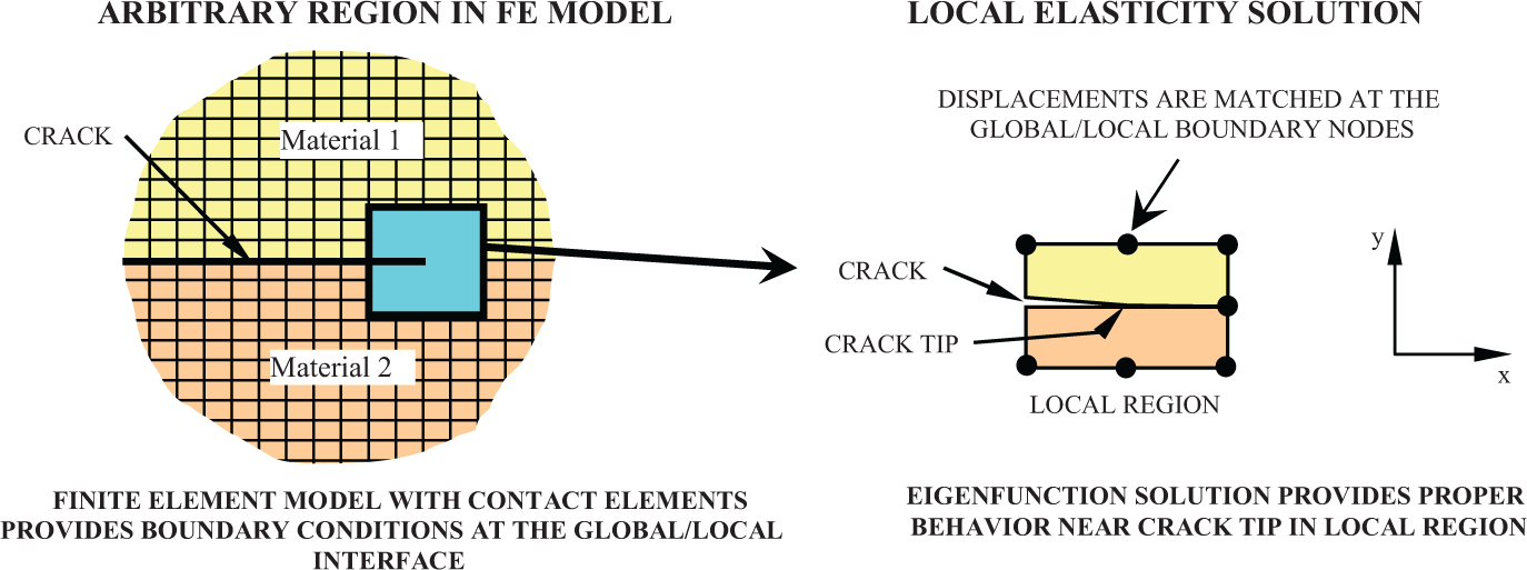
Schematic illustration of the method of analysis used.

Mathematical formulation of local elasticity solution

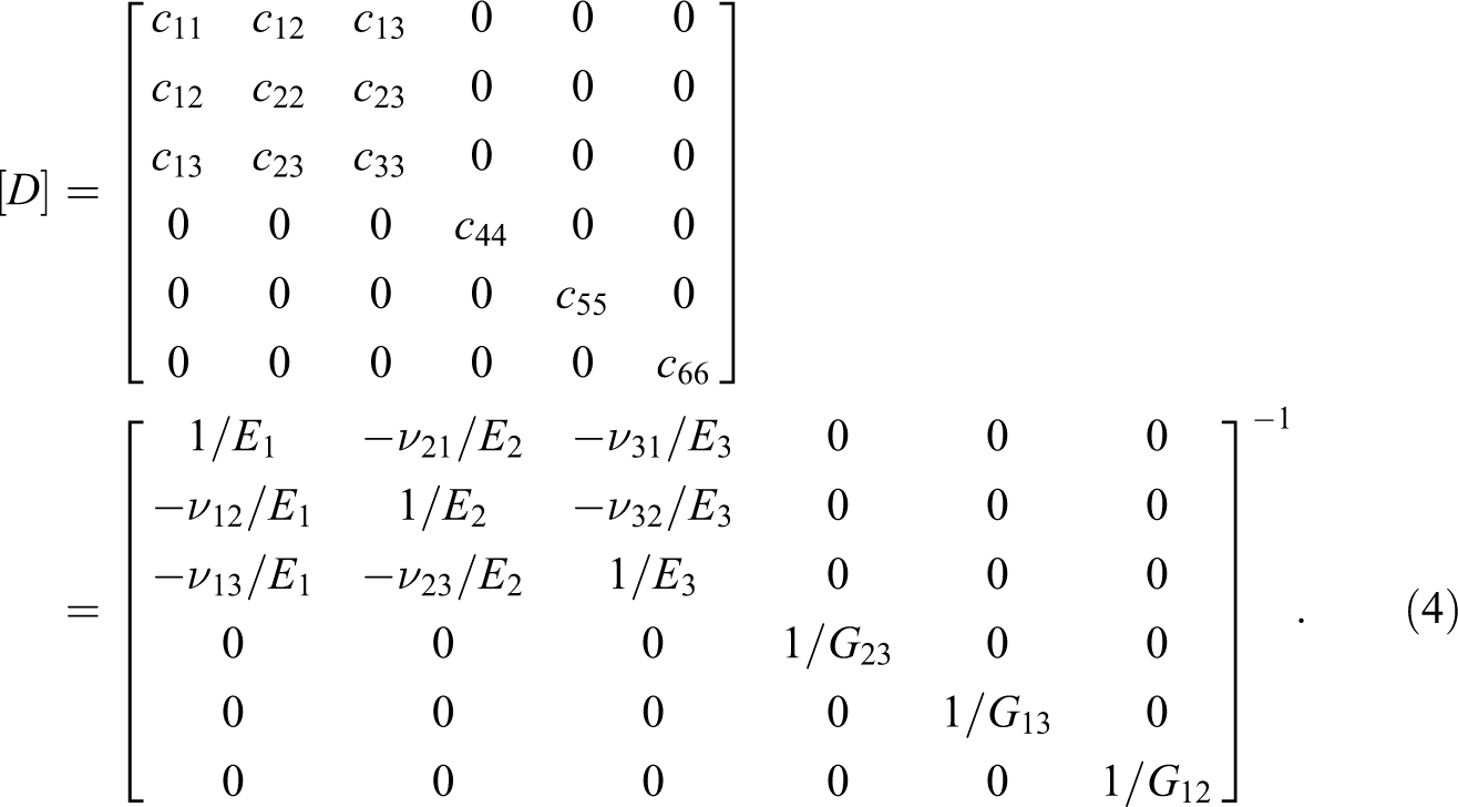
The stresses, strains, and Hooke’s law in rectangular coordinates for a linear elastic body are defined as

$\left\{\sigma \right\}=\text{stresses}={\left[\begin{array}{cccccc}{\sigma }_x& {\sigma }_y& {\sigma }_z& {\tau }_{yz}& {\tau }_{xz}& {\tau }_{xy}\end{array}\right]}^T,$

1

$\left\{\epsilon \right\}=\text{strains}={\left[\begin{array}{cccccc}{\epsilon }_x& {\epsilon }_y& {\epsilon }_z& {\gamma }_{yz}& {\gamma }_{xz}& {\gamma }_{xy}\end{array}\right]}^T,$

2

$\text{Hooke’s law:}\left\{\sigma \right\}=\left[D\right]\left\{\epsilon \right\},$

3

where, if we let E_i , ν_ij , and G_ij (i, j = 1,2,3) be the usual engineering constants, we have for orthotropic materials

$\left[D\right]=\left[\begin{array}{cccccc}{c}_{11}& c_{12}& c_{13}& 0& 0& 0\\ c_{12}& c_{22}& c_{23}& 0& 0& 0\\ c_{13}& c_{23}& c_{33}& 0& 0& 0\\ 0& 0& 0& c_{44}& 0& 0\\ 0& 0& 0& 0& c_{55}& 0\\ 0& 0& 0& 0& 0& c_{66}\end{array}\right]={\left[\begin{array}{cccccc}1/E_1& -{\nu }_{21}/E_2& -{\nu }_{31}/E_3& 0& 0& 0\\ -{\nu }_{12}/E_1& 1/E_2& -{\nu }_{32}/E_3& 0& 0& 0\\ -{\nu }_{13}/E_1& -{\nu }_{23}/E_2& 1/E_3& 0& 0& 0\\ 0& 0& 0& 1/G_{23}& 0& 0\\ 0& 0& 0& 0& 1/G_{13}& 0\\ 0& 0& 0& 0& 0& 1/G_{12}\end{array}\right]}^{-1}.$

4

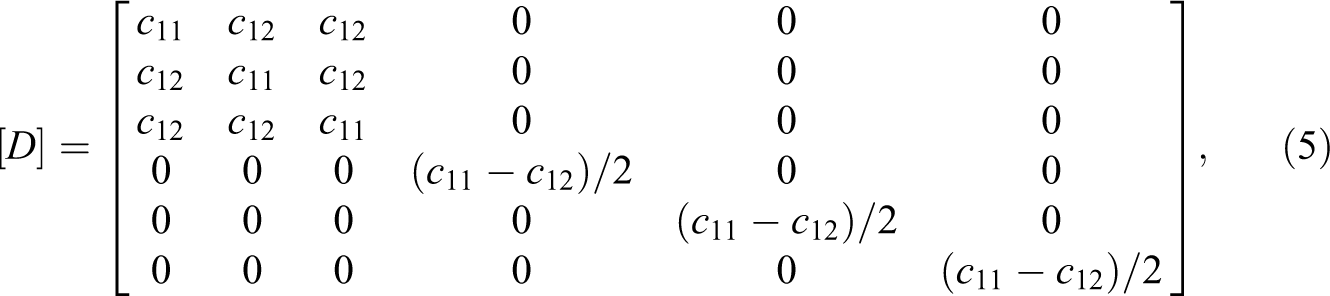
For the special case of isotropic materials with E ₁ = E ₂ = E ₃ = E. ν ₂₃ = ν ₁₃ = ν ₁₂ = ν and G ₂₃ = G ₁₃ = G ₁₂ = G = E/[2(1+ν)], we obtain

$\left[D\right]=\left[\begin{array}{cccccc}{c}_{11}& c_{12}& c_{12}& 0& 0& 0\\ c_{12}& c_{11}& c_{12}& 0& 0& 0\\ c_{12}& c_{12}& c_{11}& 0& 0& 0\\ 0& 0& 0& (c_{11}-c_{12})/2& 0& 0\\ 0& 0& 0& 0& (c_{11}-c_{12})/2& 0\\ 0& 0& 0& 0& 0& (c_{11}-c_{12})/2\end{array}\right],$

5

where

$c_{11}=\frac{(1-\nu )E}{(1+\nu )(1-2\nu )}\text{and}{c}_{12}=\frac{\nu E}{(1+\nu )(1-2\nu )}.$

6

Assuming plane strain conditions, the strain–displacement and equilibrium equations are given by

${\epsilon }_x=\frac{\partial u}{\partial x};{\epsilon }_y=\frac{\partial v}{\partial y};{\epsilon }_z=0;{\gamma }_{yz}=\frac{\partial w}{\partial y};{\gamma }_{xz}=\frac{\partial w}{\partial x};{\gamma }_{xy}=\frac{\partial u}{\partial y}+\frac{\partial v}{\partial x}.$

7

$\frac{\partial {\sigma }_x}{\partial x}+\frac{\partial {\tau }_{xy}}{\partial y}=0;\frac{\partial {\tau }_{xy}}{\partial x}+\frac{\partial {\sigma }_y}{\partial y}=0;\frac{\partial {\tau }_{xz}}{\partial x}+\frac{\partial {\tau }_{yz}}{\partial y}=0.$

8

Replacing equation (7) into equation (3) and equation (8) provides the equilibrium equations in terms of displacements as follows:

$\begin{array}{c}{c}_{11}\frac{{\partial }^{2}u}{\partial x^2}+c_{12}\frac{{\partial }^{2}v}{\partial x\partial y}+c_{66}\left(\frac{{\partial }^{2}u}{\partial y^2}+\frac{{\partial }^{2}v}{\partial x\partial y}\right)=0\\ c_{66}\left(\frac{{\partial }^{2}u}{\partial x\partial y}+\frac{{\partial }^{2}v}{\partial x^2}\right)+c_{12}\frac{{\partial }^{2}u}{\partial x\partial y}+c_{22}\frac{{\partial }^{2}v}{\partial y^2}=0\\ c_{55}\frac{{\partial }^{2}w}{\partial x^2}+c_{44}\frac{{\partial }^{2}w}{\partial y^2}=0\end{array},$

9

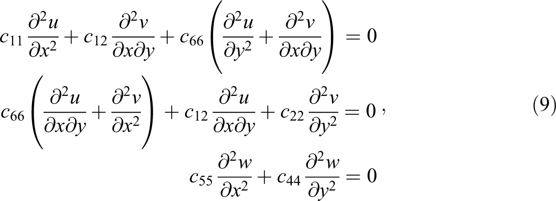
where we note that the equations for u and v are decoupled from that for w. The first two of equations (9) correspond to the in-plane problem and the third to the out-of-plane problem. In the present work, only the in-plane problem will be considered. Based on the results from Penado ¹⁰ and Ting and Chou, ¹¹ we can assume that the solution to the in-plane problem in the vicinity of the crack tip is given by

$u={\zeta }_x\left(\frac{Z_p^{1+{\lambda }_p}}{1+{\lambda }_p}\right),v={\zeta }_y\left(\frac{Z_p^{1+{\lambda }_p}}{1+{\lambda }_p}\right),$

10

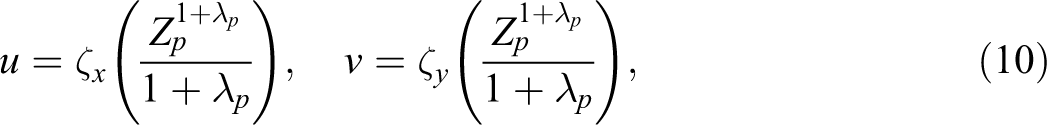
where Z_p = x + μ_py, μ_p represents the eigenvalues of the elasticity constants to be determined from the equilibrium equation (4), ζ_x and ζ_y are functions of μ_p , and λ_p are eigenvalues to be determined from the boundary conditions near the crack tip. Substituting equation (10) into the first two of equation (9) leads to the following homogeneous system of equations:

$\left[\begin{array}{cc}{c}_{11}+c_{66}{\mu }_p^2& (c_{12}+c_{66}){\mu }_p\\ (c_{12}+c_{66}){\mu }_p& c_{66}+c_{22}{\mu }_p^2\end{array}\right]\left\{\begin{array}{c}{\zeta }_x\\ {\zeta }_y\end{array}\right\}=\left\{\begin{array}{c}0\\ 0\end{array}\right\}.$

11

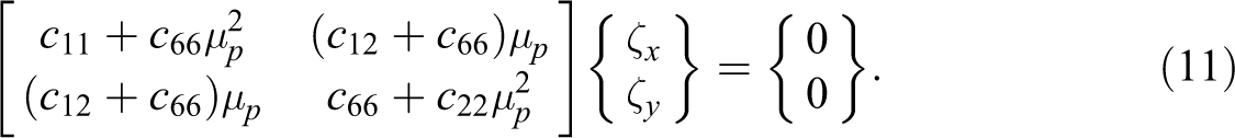
For a nontrivial solution of these equations, the determinant of the matrix of coefficients must be zero. This leads to the following quartic equation in μ_p :

$c_{22}{c}_{66}{\mu }_p^4+(c_{11}{c}_{22}-2c_{12}{c}_{66}-c_{12}^2){\mu }_p^2+c_{11}{c}_{66}=0.$

12

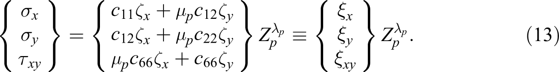
It can be shown ¹¹ that the μ‘s can only be complex or purely imaginary. Therefore, we have two complex conjugate pairs for μ_p . Once the μ_p ’s are known, ζ_x and ζ_y can be found from equation (11) up to arbitrary multiplicative constants. Now, substituting equation (10) into equations (7) and (3) gives:

$\left\{\begin{array}{c}{\sigma }_x\\ {\sigma }_y\\ {\tau }_{xy}\end{array}\right\}=\left\{\begin{array}{c}{c}_{11}{\zeta }_x+{\mu }_p{c}_{12}{\zeta }_y\\ c_{12}{\zeta }_x+{\mu }_p{c}_{22}{\zeta }_y\\ {\mu }_p{c}_{66}{\zeta }_x+c_{66}{\zeta }_y\end{array}\right\}{Z}_p^{{\lambda }_p}\equiv \left\{\begin{array}{c}{\xi }_x\\ {\xi }_y\\ {\xi }_{xy}\end{array}\right\}{Z}_p^{{\lambda }_p}.$

13

It should be noted that in the special case of an isotropic material in the x–y plane having E ₁ = E ₂ = E, ν ₁₂ = ν ₂₁ = ν, and G ₁₂ = G = E/[2(1+ν)], the conjugate pair ${\mu }_p=\pm i=\pm \sqrt{-1}$ is a double root of equation (13), and the new solution cannot be obtained by simply inserting isotropic material properties into the equations. In this case, the in-plane displacements given by equation (10) become ¹¹

$u={\zeta }_x\left(\frac{Z_p^{1+{\lambda }_p}}{1+{\lambda }_p}\right)+\frac{1}{1+{\lambda }_p}\frac{d}{d{\mu }_p}\left({\zeta }_x{Z}^{1+{\lambda }_p}\right),v={\zeta }_y\left(\frac{Z_p^{1+{\lambda }_p}}{1+{\lambda }_p}\right)+\frac{1}{1+{\lambda }_p}\frac{d}{d{\mu }_p}\left({\zeta }_y{Z}^{1+{\lambda }_p}\right).$

14

The complete asymptotic solutions for displacements and stresses near the crack tip can be obtained by taking linear combinations of the individual solutions to the first two of equations (9) corresponding to the different eigenvalues μ_p (summations over k), and λ_p (summations over m), where k and m are defined below. This leads to the following expressions for the displacements and stresses (note that the results have been converted to cylindrical coordinates with x = rcosθ and y = rsin θ):

$u_r^{(i)}={\displaystyle \sum _{m=1}^M{a}_m\left[\frac{r^{1+{({\lambda }_p)}_m}}{1+{({\lambda }_p)}_m}{\displaystyle \sum _{k=1}^4{A}_{km}^{(i)}{(F_r^{(i)})}_{km}}\right]},$

15

$u_{\theta }^{(i)}={\displaystyle \sum _{m=1}^M{a}_m\left[\frac{r^{1+{({\lambda }_p)}_m}}{1+{({\lambda }_p)}_m}{\displaystyle \sum _{k=1}^4{A}_{km}^{(i)}{(F_{\theta }^{(i)})}_{km}}\right]}$

16

${\sigma }_r^{(i)}={\displaystyle \sum _{m=1}^M{a}_m\left[r^{{({\lambda }_p)}_m}{\displaystyle \sum _{k=1}^4{A}_{km}^{(i)}{(G_r^{(i)})}_{km}}\right]},$

17

${\sigma }_{\theta }^{(i)}={\displaystyle \sum _{m=1}^M{a}_m\left[r^{{({\lambda }_p)}_m}{\displaystyle \sum _{k=1}^4{A}_{km}^{(i)}{(G_{\theta }^{(i)})}_{km}}\right]}$

18

${\tau }_{r\theta }^{(i)}={\displaystyle \sum _{m=1}^M{a}_m\left[r^{{({\lambda }_p)}_m}{\displaystyle \sum _{k=1}^4{A}_{km}^{(i)}{(G_{r\theta }^{(i)})}_{km}}\right]},$

19

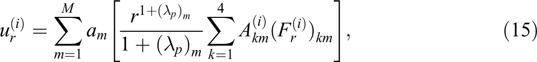
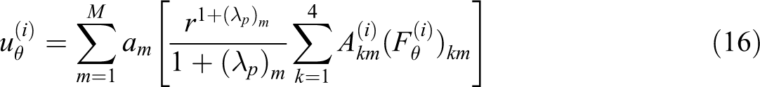
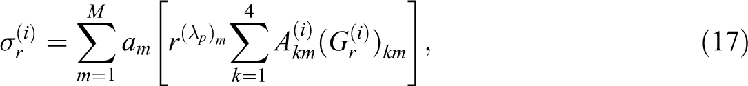
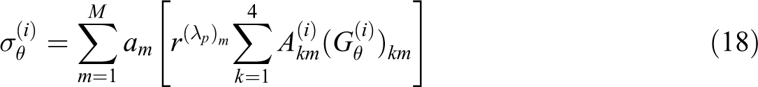
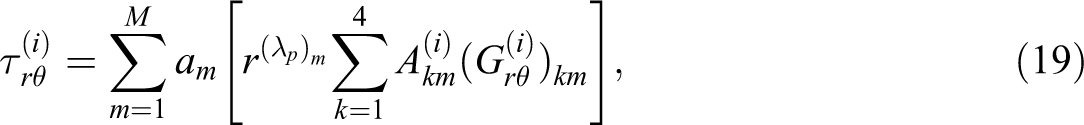
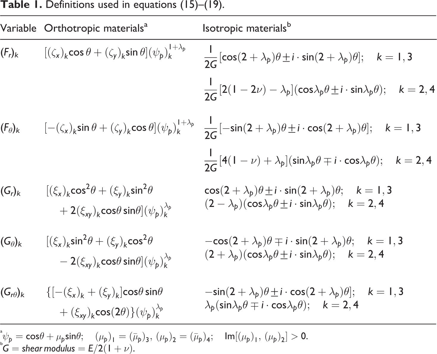
where the superscript i = 1,2 denotes each material region; k and m are dummy indices of summation associated with the eigenvalues of the problem; M is the number of terms in the truncated infinite series; a_m ’s are multiplicative constants associated with the in-plane eigenvectors; F_ij and G_ij are defined in Table 1; and (λ_p ) _m and A_km will be defined later in relation to the boundary conditions at the crack tip.

Table 1.

Definitions used in equations (15) –(19).

Variable	Orthotropic materialsa	Isotropic materialsb
(Fr ) k	$[{({\zeta }_x)}_k\text{cos}\theta +{({\zeta }_y)}_k\text{sin}\theta ]{({\psi }_p)}_k^{1+{\lambda }_p}$	$\begin{array}{l}\frac{1}{2G}[\text{cos}(2+{\lambda }_p)\theta \pm i\cdot \text{sin}(2+{\lambda }_p)\theta ];k=1,3\hfill \\ \frac{1}{2G}[2(1-2\nu )-{\lambda }_p](\text{cos}{\lambda }_p\theta \pm i\cdot \text{sin}{\lambda }_p\theta );k=2,4\hfill \end{array}$
(Fθ ) k	$[-{({\zeta }_x)}_k\text{sin}\theta +{({\zeta }_y)}_k\text{cos}\theta ]{({\psi }_p)}_k^{1+{\lambda }_p}$	$\begin{array}{l}\frac{1}{2G}[-\text{sin}(2+{\lambda }_p)\theta \pm i\cdot \text{cos}(2+{\lambda }_p)\theta ];k=1,3\hfill \\ \frac{1}{2G}[4(1-\nu )+{\lambda }_p](\text{sin}{\lambda }_p\theta \mp i\cdot \text{cos}{\lambda }_p\theta );k=2,4\hfill \end{array}$
(Gr ) k	$[{({\xi }_x)}_k{\text{cos}}^2\theta +{({\xi }_y)}_k{\text{sin}}^2\theta +2{({\xi }_{xy})}_k\text{cos}\theta \text{sin}\theta ]{({\psi }_p)}_k^{{\lambda }_p}$	$\begin{array}{l}\text{cos}(2+{\lambda }_p)\theta \pm i\cdot \text{sin}(2+{\lambda }_p)\theta ;k=1,3\hfill \\ (2-{\lambda }_p)(\text{cos}{\lambda }_p\theta \pm i\cdot \text{sin}{\lambda }_p\theta );k=2,4\hfill \end{array}$
(Gθ ) k	$[{({\xi }_x)}_k{\text{sin}}^2\theta +{({\xi }_y)}_k{\text{cos}}^2\theta -2{({\xi }_{xy})}_k\text{cos}\theta \text{sin}\theta ]{({\psi }_p)}_k^{{\lambda }_p}$	$\begin{array}{l}-\text{cos}(2+{\lambda }_p)\theta \mp i\cdot \text{sin}(2+{\lambda }_p)\theta ;k=1,3\hfill \\ (2+{\lambda }_p)(\text{cos}{\lambda }_p\theta \pm i\cdot \text{sin}{\lambda }_p\theta );k=2,4\hfill \end{array}$
(Grθ ) k	$\{[-{({\xi }_x)}_k+{({\xi }_y)}_k]\text{cos}\theta \text{sin}\theta +{({\xi }_{xy})}_k\text{cos}(2\theta )\}{({\psi }_p)}_k^{{\lambda }_p}$	$\begin{array}{l}-\text{sin}(2+{\lambda }_p)\theta \pm i\cdot \text{cos}(2+{\lambda }_p)\theta ];k=1,3\hfill \\ {\lambda }_p(\text{sin}{\lambda }_p\theta \mp i\cdot \text{cos}{\lambda }_p\theta );k=2,4\hfill \end{array}$

^a ${\psi }_p=\text{cos}\theta +{\mu }_p\text{sin}\theta ;{({\mu }_p)}_1={({\overline{\mu }}_p)}_3,{({\mu }_p)}_2={({\overline{\mu }}_p)}_4;\text{\hspace{1em}Im}[{({\mu }_p)}_1,{({\mu }_p)}_2]>0$ .

^b $G=shearmodulus=E/2(1+\nu )$ .

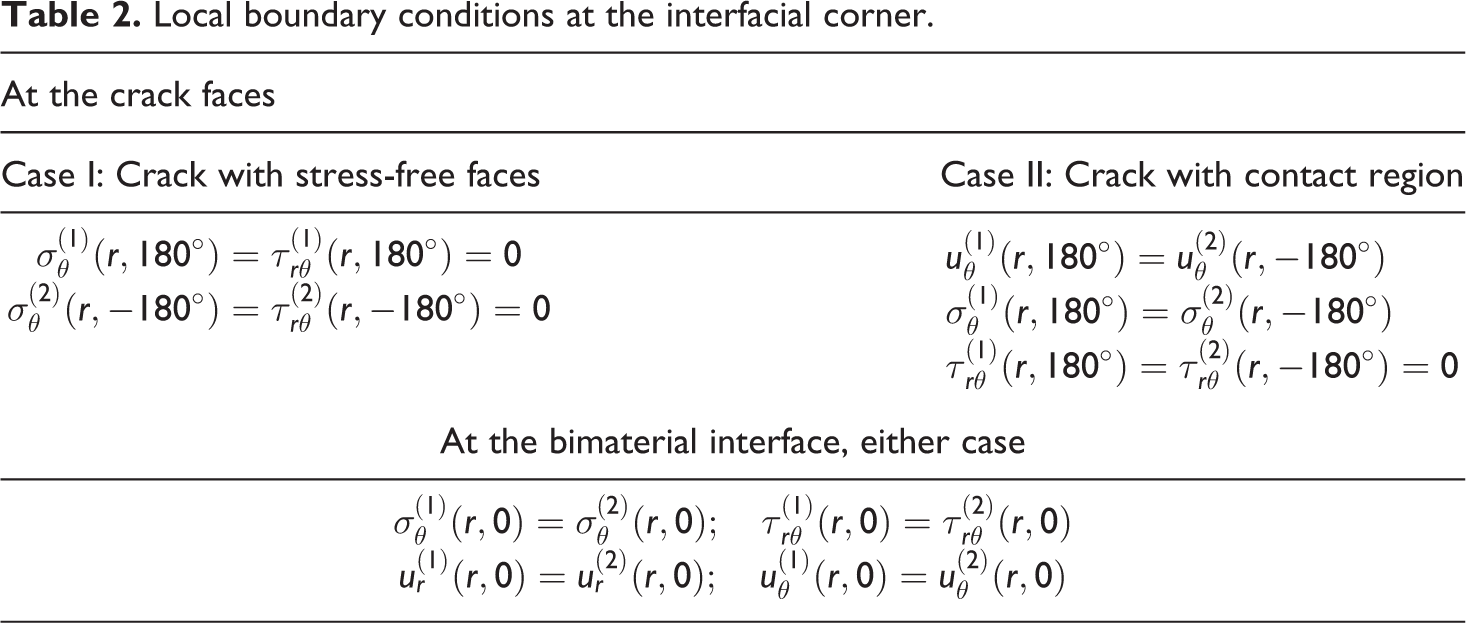
Two types of boundary conditions must be considered to find all of the unknown parameters: local and remote. The local boundary conditions provide (λ_p ) _m and A_km and depend on whether the crack faces are stress-free or a contact region near the crack tip exists. In the present problem, either condition may exist depending on the crack length and material properties; this is discussed in more detail later in the article. The appropriate local boundary conditions for either case are shown in Table 2 and Figure 2. In case II, frictionless contact at the crack faces has been assumed.

Table 2.

Local boundary conditions at the interfacial corner.

At the crack faces
Case I: Crack with stress-free faces	Case II: Crack with contact region
$\begin{array}{c}{\sigma }_{\theta }^{(1)}(r,180°)={\tau }_{r\theta }^{(1)}(r,180°)=0\\ {\sigma }_{\theta }^{(2)}(r,-180°)={\tau }_{r\theta }^{(2)}(r,-180°)=0\end{array}$	$\begin{array}{c}{u}_{\theta }^{(1)}(r,180°)=u_{\theta }^{(2)}(r,-180°)\\ {\sigma }_{\theta }^{(1)}(r,180°)={\sigma }_{\theta }^{(2)}(r,-180°)\\ {\tau }_{r\theta }^{(1)}(r,180°)={\tau }_{r\theta }^{(2)}(r,-180°)=0\end{array}$
At the bimaterial interface, either case
$\begin{array}{c}{\sigma }_{\theta }^{(1)}(r,0)={\sigma }_{\theta }^{(2)}(r,0);{\tau }_{r\theta }^{(1)}(r,0)={\tau }_{r\theta }^{(2)}(r,0)\\ u_r^{(1)}(r,0)=u_r^{(2)}(r,0);u_{\theta }^{(1)}(r,0)=u_{\theta }^{(2)}(r,0)\end{array}$

Figure 2.

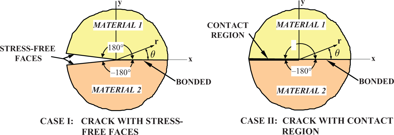
Local boundary conditions near the crack tip.

Substitution of equations (15) –(19) into the appropriate equations from Table 2 leads to a homogeneous system of linear equations:

$r^{{\lambda }_p}\left[K_p({\lambda }_p)\right]\left\{A\right\}=\left\{0\right\},$

20

where [K_p (λ_p )] is an 8 × 8 matrix with entries that depend on λ_p , and {A} is an 8 × 1 matrix defined as follows:

$\left\{A\right\}={\left[\begin{array}{cccccccc}{A}_1^{(1)}& A_2^{(1)}& A_3^{(1)}& A_4^{(1)}& A_1^{(2)}& A_2^{(2)}& A_3^{(2)}& A_4^{(2)}\end{array}\right]}^T.$

21

For nontrivial solutions to equation (20), its determinant of coefficients must be zero:

$\left|K_p({\lambda }_p)\right|=0.$

22

The solution of equation (22) leads to an infinite number of roots λ_p . These roots were found by truncating the system and using a nonlinear equation solver. ¹² Then, with the roots known, the eigenvector {A} in equation (20) was found by using singular value decomposition. ^13,14 This process, however, only defines the eigenvectors up to arbitrary multiplicative constants (a_m in equations (15) –(19)). These constants were determined from the remote boundary conditions of the model at the global/local interface, as discussed next.

Remote boundary conditions

The determination of the multiplicative constants a_m requires the application of the remote boundary conditions at the global/local interface. This is done by matching displacements of the local and global solutions at the interface (see Figure 1). In the global solution, a nonlinear finite element model with contact elements was used to avoid interpenetration of the crack faces and determine the extent of the contact region. This way, the appropriate case from Table 2 for the local region was selected. Furthermore, the best results from this match are achieved by using more boundary stations than unknown constants. ^{15 –17} The resulting overdetermined system of equations was satisfied in the present work in a least squares sense by using singular value decomposition. ^13,14 A total of M = 30 terms were used in the eigenfunction expansion, which resulted in an error of less than 2% in satisfying the remote boundary conditions. The error was calculated as the largest element of the residual divided by the maximum boundary displacement, where the residual is the mismatch between the truncated eigenfunction series and the remote traction boundary conditions.

Approximate model of global region

The problem analyzed consists of a plate with a central crack at the interface of two isotropic or orthotropic materials and subjected to a combination of axial and shear loading. This configuration was chosen in order to be able to compare directly with results in the literature for the special case of isotropic materials. Thus, the displacement field in the plate at the boundary of the local region was found by using the finite element model shown in Figure 3. The plate had overall dimensions of 177.8 × 203.2 mm with a crack length of 25.4 mm. The analysis was conducted using the COSMOS/M finite element code ¹⁸ and consisted of 6000 eight-noded quadrilateral plane strain elements and 18,400 nodes. In addition, 79 nonlinear gap elements were used at the crack faces to simulate the contact problem and avoid interpenetration. The element size in the crack region in the x- and y-directions was, respectively, 0.635 and 1.27 mm. Tensile loading was applied by constraining the bottom edge of the plate from displacements in the y-direction, while forces were applied on the top edge. Shear loading was achieved by tangential and self-equilibrating forces on opposite edges, as shown in Figure 3. For isotropic materials, the properties for material 1 used were E = 10 × 10⁶ psi and ν = 0.3, while the properties of material 2 were varied to produce a range of Dundurs parameter, which for plane strain is defined as ⁴

$\beta =\text{Dundurs\hspace{0.17em}parameter}=\frac{1}{2}\frac{G_1(1-2{\nu }_2)-G_2(1-2{\nu }_1)}{G_1(1-{\nu }_2)+G_2(1-{\nu }_1)},$

23

Figure 3.

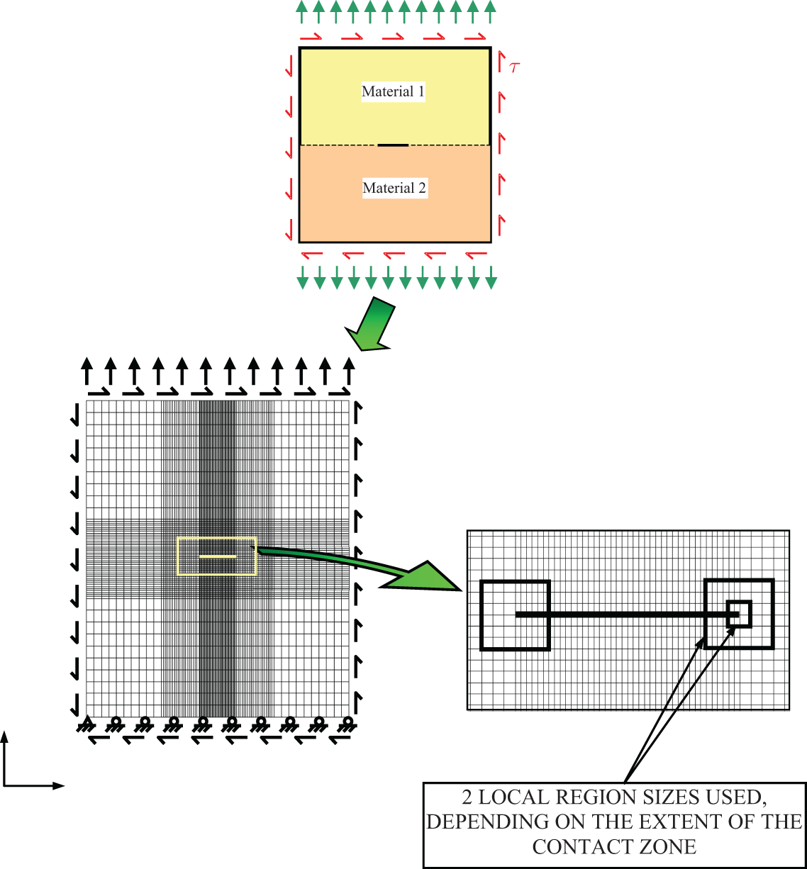
Mesh, loading and boundary conditions used in the global finite element analysis.

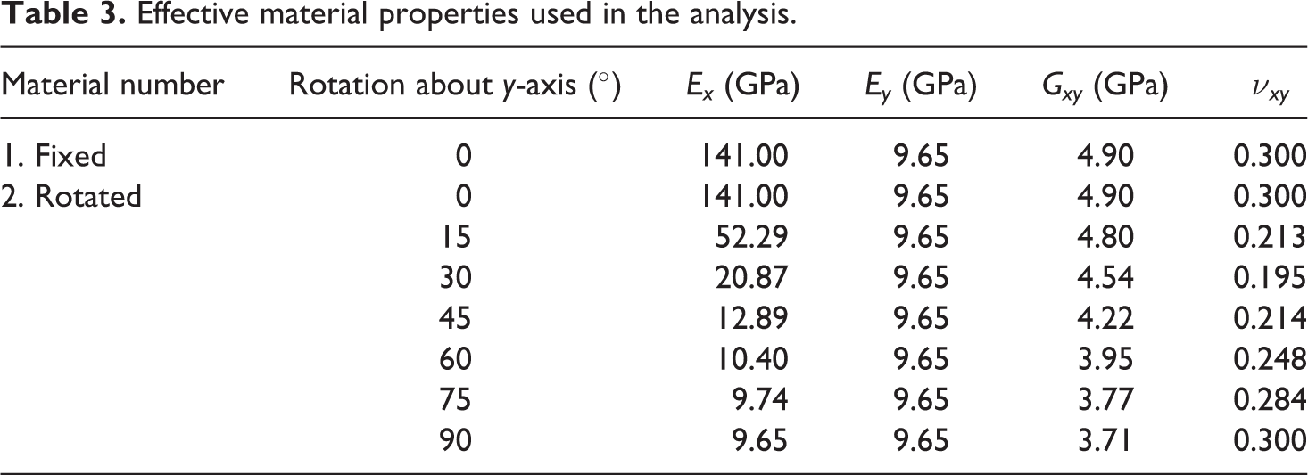
where G = shear modulus = E/[2(1+ν)], E = Young’s modulus, ν = Poisson’s ratio, and the subscript i = 1,2 refers to the material number. Note that the sign of β is reversed when materials 1 and 2 are exchanged. For orthotropic materials, the material variation used corresponds to the angle of rotation of a unidirectional composite ply about the y-axis. It should be noted, however, that for angles other than 0° and 90°, coupling of in-plane and out-of-plane effects occurs. However, the out-of-plane coupling effects caused by off-axis plies can be neglected, and effective ply moduli can be used as a close approximation, as shown by Penado. ¹⁹ The resulting effective properties used are shown in Table 3.

Table 3.

Effective material properties used in the analysis.

Material number	Rotation about y-axis (°)	Ex (GPa)	Ey (GPa)	Gxy (GPa)	νxy
1. Fixed	0	141.00	9.65	4.90	0.300
2. Rotated	0	141.00	9.65	4.90	0.300
	15	52.29	9.65	4.80	0.213
	30	20.87	9.65	4.54	0.195
	45	12.89	9.65	4.22	0.214
	60	10.40	9.65	3.95	0.248
	75	9.74	9.65	3.77	0.284
	90	9.65	9.65	3.71	0.300

Contact region of crack

The extent of the contact region was found directly from the finite element results. A typical deformed mesh showing a partially closed crack is given in Figure 4. The extent of the contact zone is defined in Figure 5 by the parameter b. The limiting values are b/L = 1 for a completely open crack and b/L = −1 for a completely closed crack. In general, for a given value of the ratio of axial to shear stress, σ/τ, two distinct contact regions can be observed: large and small. These two regions are discussed separately next.

Figure 4.

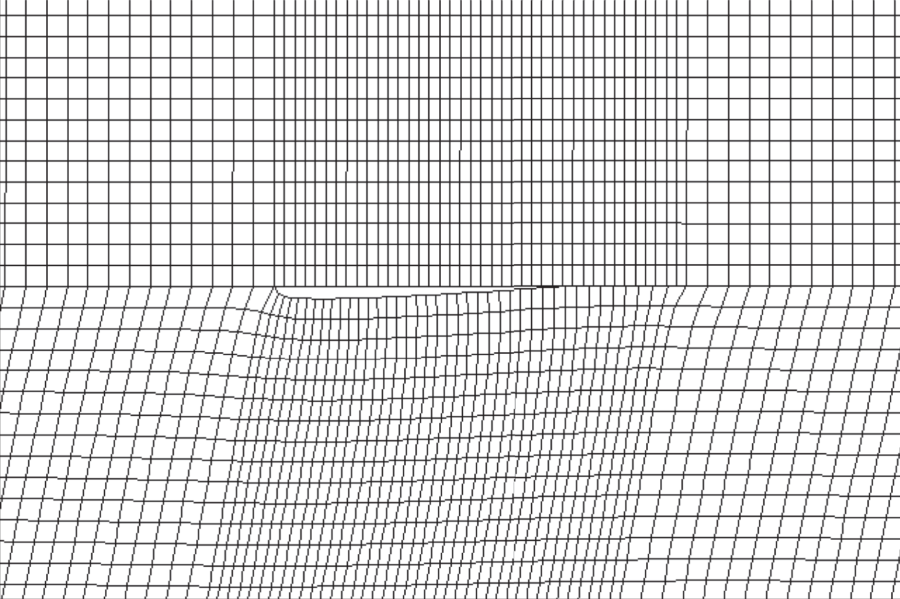
Typical deformed mesh showing a partially closed crack at the interface between two isotropic materials. The case shown corresponds to σ/τ = 0.2 and β = 0.5.

Figure 5.

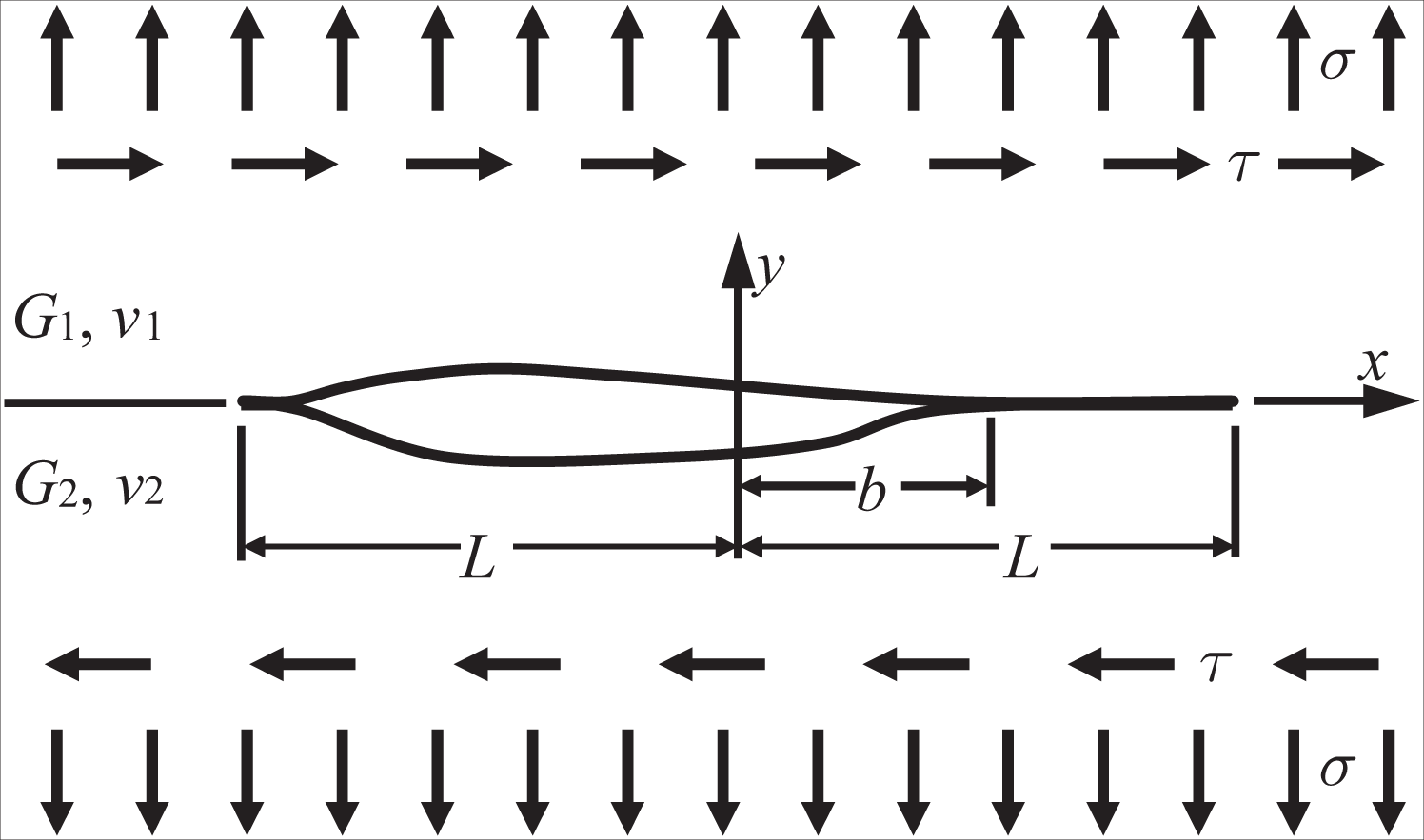
Notation used in relation to partially closed crack.

Large contact region

On the right end of the crack, a large contact region occurs which has length L−b, as defined by Figure 5. Results for the contact region as a function of the stress ratio, σ/τ, and the Dundurs parameter, β, are given in Figure 6 for the isotropic case and are compared with results from Gautesen and Dundurs. ⁴ Close agreement is seen in all cases, indicating the validity of the finite element model used. Similar results for the orthotropic case are given in Figure 7. It is interesting to note that for the case of pure shear (σ/τ = 0), the contact zone is almost constant with layup angle. A similar trend of nearly constant contact zone with Dundurs parameter is also observed for isotropic materials in pure shear (Figure 6).

Figure 6.

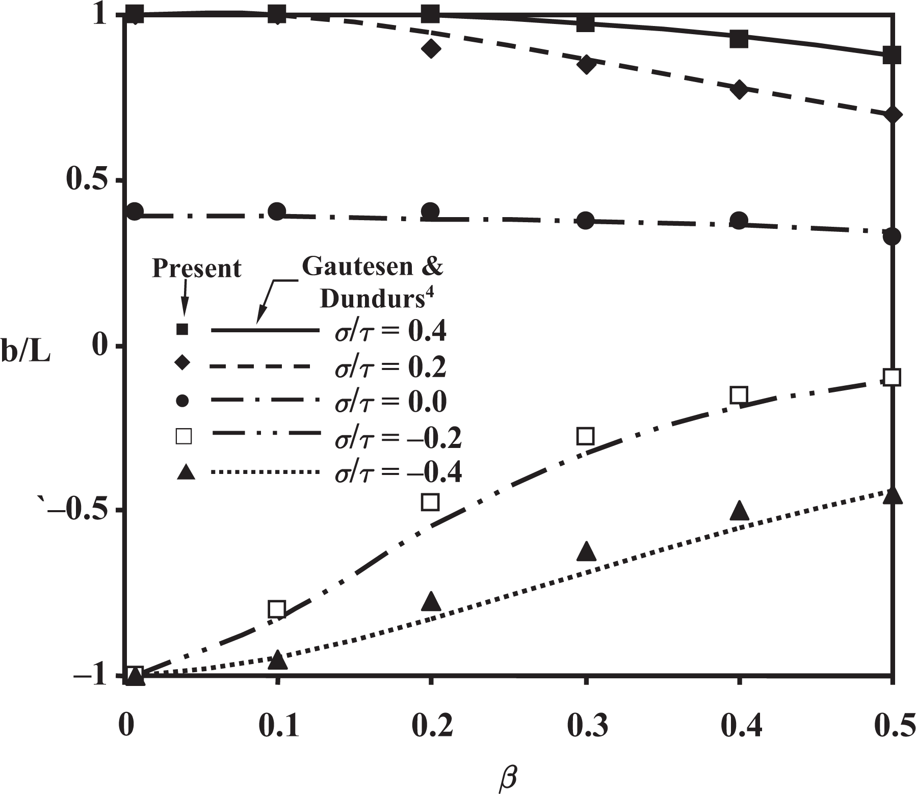
Comparison of present results with Gautesen and Dundurs ⁴ for the extent of the large contact zone (right tip).

Figure 7.

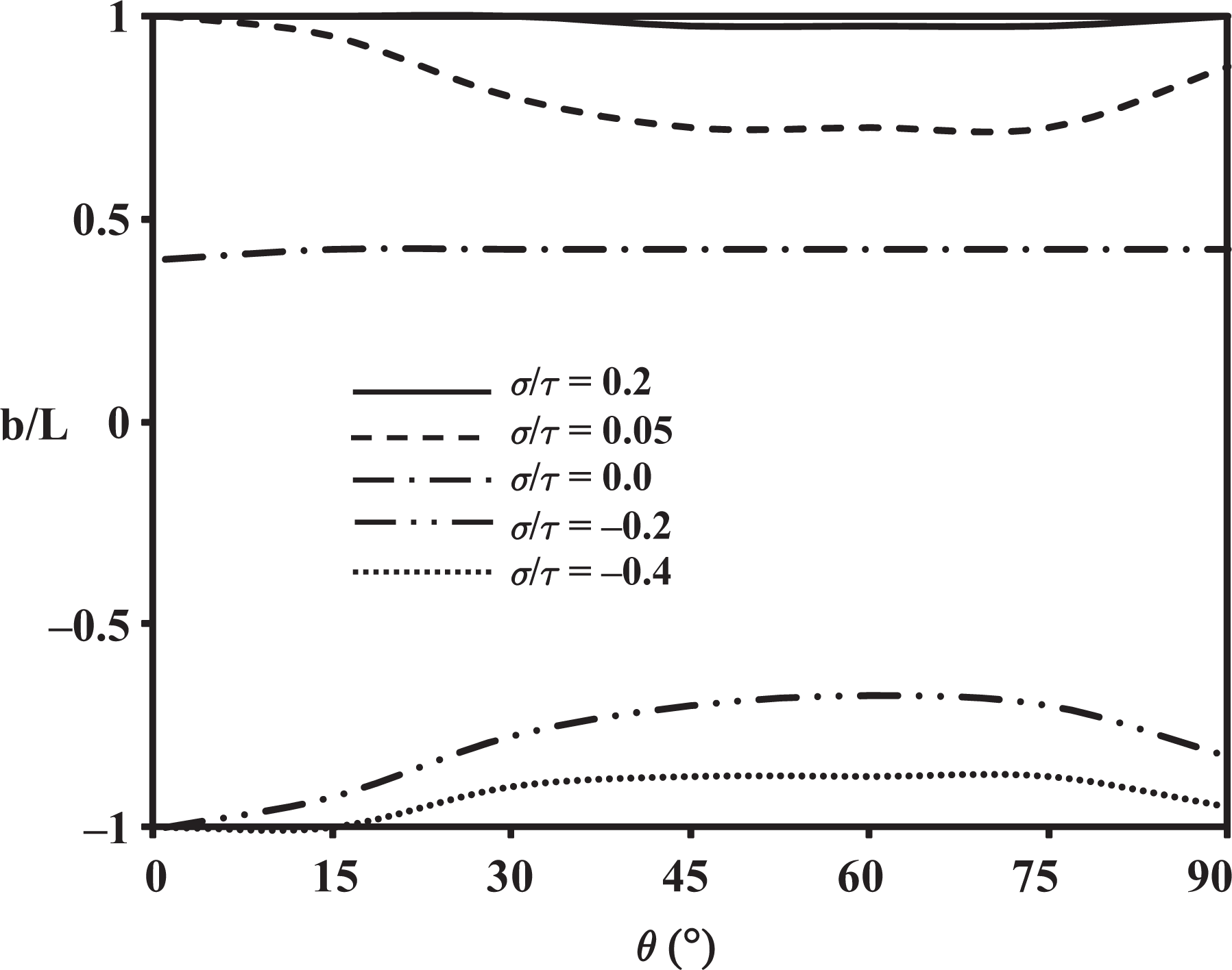
Extent of the large contact zone (right tip) for orthotropic materials having the properties defined in Table 3.

Small contact region

The results in Figures 6 and 7 correspond to the large contact zone that appears on the right crack tip. On the opposite (left) crack tip, a very small contact region, of the order of 10^–8 of the crack length, appears. ⁴ The finite element model, however, does not reveal this contact zone when the element size is larger than the contact region, and in these cases, the finite element results appear to indicate that the crack is completely open at this location (see Figure 4). However, the existence of the small contact zone can be inferred from the local elasticity solution using the completely open crack boundary conditions (case I in Table 2). In this case, the singular eigenvalue, which is that having Re(λ_p )<0, from equation (22) is complex, indicating oscillatory stresses and overlapping displacements near the crack tip, which is physically inadmissible; therefore, a contact zone must be present. On the other hand, for the large contact region, the singular eigenvalue is real and the finite element results clearly show a contact zone. The calculation of the stress intensity factor for the small contact zone was treated approximately, as shown next.

Approximate analysis of the interfacial crack with a small contact region

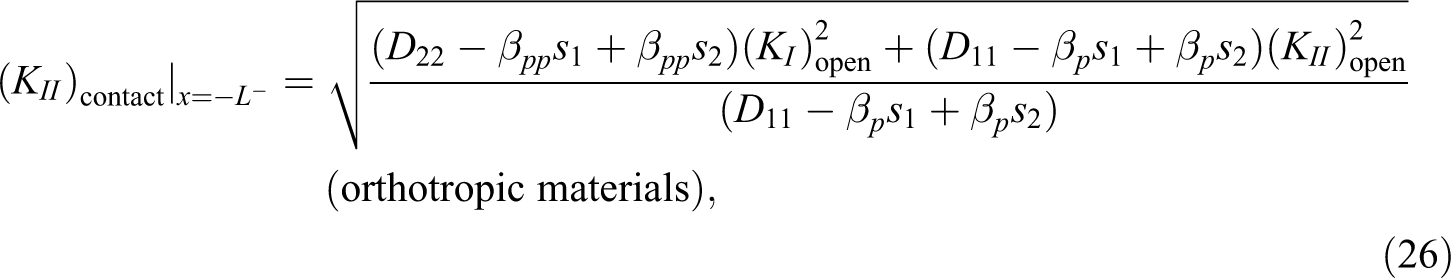
For the left tip, where the crack appears open (e.g., Figure 4) but the singular eigenvalue is complex, a very small contact region appears, the extent of which cannot be determined directly from the finite element results. The maximum extent of this region is typically on the order of 10^–8 of the crack length. ⁴ In these cases, it has been shown by Penado ² that the results for the stress intensity factor can be approximated by considering the J-integral in combination with the results assuming stress free crack faces (case I in Figure 2 and Table 2). The results for the small contact region stress intensity factors just to the left of the crack tip in terms of the open crack values are ²

${{(K_I)}_{\text{contact}}|}_{x=-L^{-}}=0\text{\hspace{0.17em}(isotropic or orthotropic materials),}$

24

${{(K_{II})}_{\text{contact}}|}_{x=-L^{-}}=\sqrt{{(K_I)}_{\text{open}}^2+{(K_{II})}_{\text{open}}^2}\text{\hspace{0.17em}(isotropic materials),}$

25

${{(K_{II})}_{\text{contact}}|}_{x=-L^{-}}=\sqrt{\frac{(D_{22}-{\beta }_{pp}{s}_1+{\beta }_{pp}{s}_2){(K_I)}_{\text{open}}^2+(D_{11}-{\beta }_p{s}_1+{\beta }_p{s}_2){(K_{II})}_{\text{open}}^2}{(D_{11}-{\beta }_p{s}_1+{\beta }_p{s}_2)}}\text{ (orthotropic materials),}$

26

where

$\begin{array}{cc}{D}_{11}=\frac{s_1}{{\eta }_1}+\frac{s_2}{{\eta }_2}& D_{22}=\frac{s_1{\rho }_1}{{\eta }_1}+\frac{s_2{\rho }_2}{{\eta }_2}\\ s_1={\left(c_{12}^{(1)}+\sqrt{c_{11}^{(1)}{c}_{22}^{(1)}}\right)}^{-1}& s_2={\left(c_{12}^{(2)}+\sqrt{c_{11}^{(2)}{c}_{22}^{(2)}}\right)}^{-1}\\ {\rho }_1=\sqrt{c_{11}^{(1)}/c_{22}^{(1)}}& {\rho }_2=\sqrt{c_{11}^{(2)}/c_{22}^{(2)}}\\ {\eta }_1=\sqrt{\frac{c_{66}^{(1)}\left(\sqrt{c_{11}^{(1)}{c}_{22}^{(1)}}-c_{12}^{(1)}\right)}{c_{22}^{(1)}\left(2c_{66}^{(1)}+c_{12}^{(1)}+\sqrt{c_{11}^{(1)}{c}_{22}^{(1)}}\right)}}& {\eta }_2=\sqrt{\frac{c_{66}^{(2)}\left(\sqrt{c_{11}^{(2)}{c}_{22}^{(2)}}-c_{12}^{(2)}\right)}{c_{22}^{(2)}\left(2c_{66}^{(2)}+c_{12}^{(2)}+\sqrt{c_{11}^{(2)}{c}_{22}^{(2)}}\right)}}\\ {\beta }_p=\frac{s_1-s_2}{D_{22}}& {\beta }_{pp}=\frac{s_1-s_2}{D_{11}}\end{array}.$

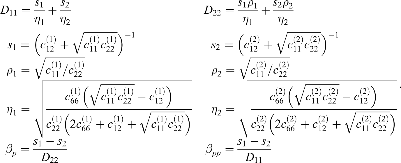
It should be noted that only the orthotropic case was considered by Penado ² ; however, the isotropic case can be found as a limiting case, since then ρ ₁ = ρ ₂ = 1, D ₁₁ = D ₂₂, and β_p = β_pp = β = Dundurs parameter.

Results and discussion

The mode I and II stress intensity factors were calculated from their definitions in terms of the parameters λ_p , {A} and a_m defined earlier, as well as F_ij and G_ij defined in Table 1:

$K_I=\left(\sqrt{2\pi }\right)a_1{\displaystyle \sum _{k=1}^4{A}_{k1}{\left(G_{\theta }{|}_{\theta =0}\right)}_{k1}};K_{II}=\left(\sqrt{2\pi }\right)a_1{\displaystyle \sum _{k=1}^4{A}_{k1}{\left(G_{r\theta }{|}_{\theta =0}\right)}_{k1}}.$

27

For complex (λ_p )₁, K_I and K_II are found by adding the terms associated with the complex conjugate pair of eigenvalues (λ_p )₁ and (λ_p )₂, which produces a real value by cancellation of the imaginary parts.

Two local region sizes were used, large and small, depending on the extent of the contact zone, as shown in Figure 3. The sizes of these zones were, respectively, 0.6 L × 0.6 L and 0.2 L × 0.2 L, centered at the crack tips. Referring to Figure 5 for nomenclature, the left tip of the crack appeared open in all cases and the large region size was used. For the right tip, in cases where a contact zone develops, the large region size was used for −1≤b/L<0.7, while the small size was used for 0.7≤b/L≤0.95. The two region sizes allow the contact zone to always be contained within the local region. Note that the dimensionless parameter b/L defines the limit of contact (see Figure 5). Additionally, in cases where the right tip appears open, b/L>0.95, the large local region size was used.

In order to validate the method, the analytical results for isotropic materials from Gautesen and Dundurs ⁴ for the dimensionless mode II stress intensity factor, K_II /[L(σ ²+τ ²)]^1/2, as a function of the Dundurs parameter, β, were compared with the present results. The results from Gautesen and Dundurs ⁴ are reproduced in Figure 8. Due to the narrow range of values of dimensionless K_II , it is difficult to make a meaningful comparison with the present results by plotting directly in Figure 8. Instead, the comparison was performed by calculating the percent error, which is shown in Figure 9. It can be seen that the error is less than 3% in most cases. The worst error was found to be −6.35% at σ/τ = 0.2, β = 0.2; however, in the vast majority of cases, the error was within 35% of exact solutions. For the present results, note that for the right tip a large contact zone exists and K_I (L) = 0 in all cases. Also, at the left tip, the singular eigenvalue for the open crack problem was found to be complex in all cases, indicating that a small contact zone was present and K_I (−L) = 0 also.

Figure 8.

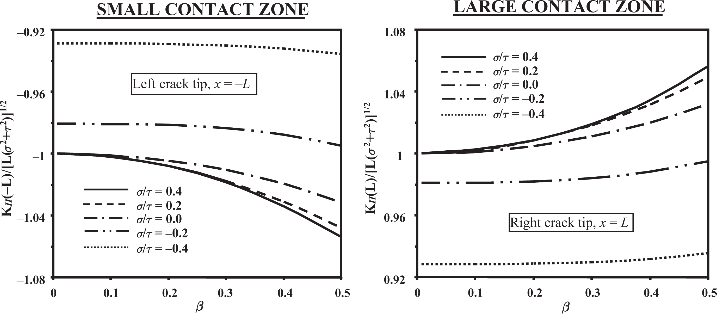
Gautesen and Dundurs ⁴ results for the dimensionless mode II stress intensity factor at the left and right crack tips, x = −L and x = L.

Figure 9.

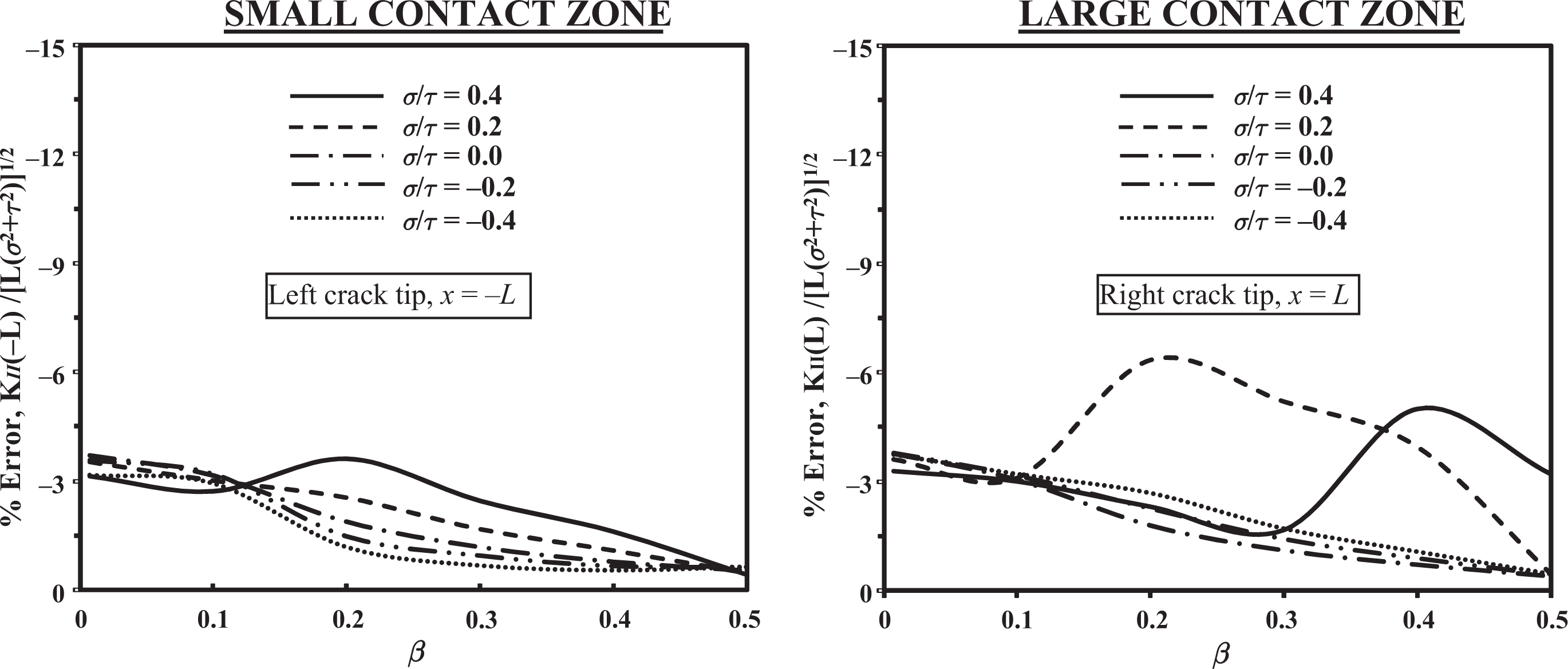
Percent error of present results with respect to values in Gautesen and Dundurs ⁴ at the left and right crack tips, x = −L and x = L.

Additionally, results for the dimensionless K_II for an orthotropic plate were obtained as a function of the angle of rotation of a unidirectional composite ply using the effective properties shown in Table 3. These results are shown in Figure 10. No corresponding results for orthotropic materials are found in the literature for comparison. For all stress ratio cases, the largest absolute values of the dimensionless K_II occur near a rotation angle of 35°, indicating that this may be a significant ply angle for delaminations in a composite laminate.

Figure 10.

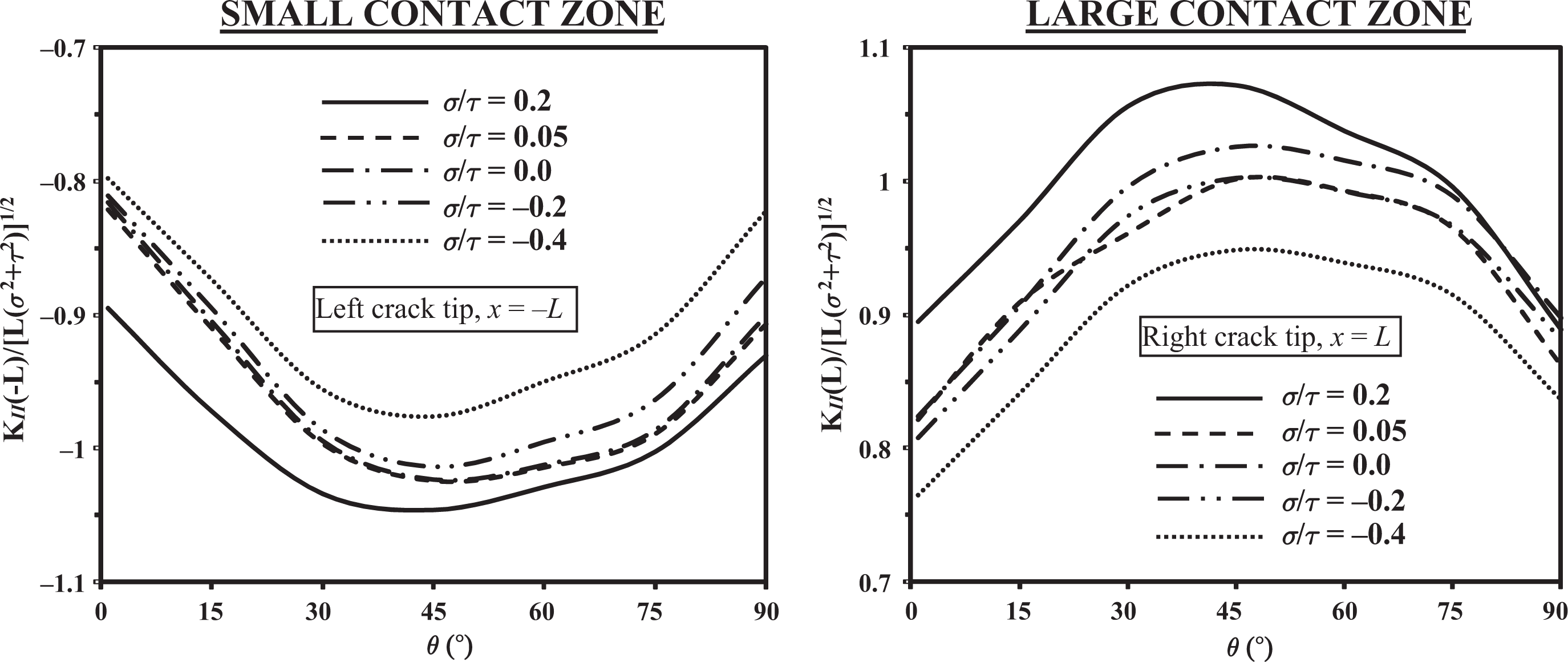
Results for the dimensionless K_II for an orthotropic plate as a function of the angle of rotation of a unidirectional composite ply.

Conclusions

A hybrid method combining finite elements and eigenfunction expansions was further examined and validated. The method allows consideration of complex geometries, materials, loading, and boundary conditions to solve fracture mechanics problems. In addition, the method is portable and requires no special finite element codes or elements. Results were shown for a variety of shear and normal loads on a cracked bimaterial plate with isotropic or orthotropic material properties and frictionless crack face contact. The results for the isotropic case were compared with closed form solutions in the literature and good agreement was found. In general, the results can be expected to be within 3–5% of exact solutions. Overall, we conclude that the method provides a practical and reliable way to analyze a variety of engineering structures with interfacial cracks.