
Abstract
In this article, a three-dimensional (3D) finite elements method has been developed for predicting the effective thermal conductivity (ETC) of a conductive hollow tube polymer composite. 3D Representative Volume Element (3D-RVE) was used to represent the composite material. Governing heat transfer equations in both transverse and longitudinal directions for predicting the effective thermal conductivities of composites are used. ETC was numerically calculated using COMSOLTM software. The guarded hot plate method was used to measure the composites conductivities consisting of epoxy resin matrix filled with metallic hollow tube. A comparison between the numerically calculated thermal conductivities, measured and analytical ones for various samples was made. A satisfactory agreement between numerical and experiment takes place.
Introduction
Various approaches for characterizing the effective thermal, electrical, and elastic properties of composite media have been introduced since Maxwell’s seminal work on spherical particle suspensions more than a century ago. 1 Apart from the large number of results, which are based on either highly approximated micro-models or ad hoc mixing rules, several approaches based on reasonable physical models have also been established and refined to include the effects of various particle shapes and of an imperfect thermal contact between the particle surface and the continuous medium. Such studies include the exact mathematical analysis of dilute systems, in which bounds are established on the effective properties, and asymptotic behavior is determined (Beasley and Torquato 2 and Thovert and Acrivos 3 ); exact mathematical analysis of various regular arrays of particles (McKenzie et al., 4 Gu and Tao, 5 Gu and Liu, 6 Torquato and Rintoul, 7 and Cheng and Torquato 8 ); numerical simulation of Brownian diffusion of pulsed sources through particle arrays (Torquato and Kim, 9 and Kim and Torquato 10 ); the self-consistent field concept for analyzing non-dilute, non-regularly spaced particles (Hashin, 11 Benveniste and Miloh, 12 and Benveniste 13 ); and the technique of successive embedding of effective media to treat multicoated cylinders or spheres (Schulgasser, 14 and Milgrom and Shtrikman 15 ).
Numerous numerical studies of thermal conductivity of filled polymer were also conducted in the past. Thus, Deissler’s works 16 were extended by Wakao and Kato 17 for a cubic or orthorhombic array of uniform spheres in contact. Shonnard and Whitaker 18 have investigated the influence of contacts on two-dimensional (2D) models. They have developed a global equation with an integral method for heat transfer in the medium. Auriault and Ene 19 have investigated the influence of the interfacial thermal barrier on the effective conductivity and on the structure of the macroscopic heat transfer equations. Using the finite elements method (FEM), Veyret et al. 20 studied the heat conductive transfer in the periodic distribution of the filler in the composite materials. In their study, calculation was carried out on 2D and 3D geometric spaces. The same method was used by Ramani and Vaidyanathan 21 , who incorporated the effect of microstructural characteristics such as filler aspect ratio, interfacial thermal resistance, volume fraction, and filler dispersion to determine the effective thermal conductivity (ETC) of a composite with spherical and parallelepiped fillers. The thermal conductivity increased from 0.32 W m−1 K−1 for pure PA6 to 2.09 W m−1 K−1 by adding spherical copper powder filler with a 50% volume fraction. Terada et al. 22 have generated an FEM by identifying each pixel with a finite element and accompanying appropriate image processing. Bakker 23 has calculated the thermal conductivity coefficient of porous materials by using FEM and has looked for the relationship between 2D and 3D values. A numerical approach to calculate the ETC of granular-reinforced composite was proposed by Cruz. 24 Many other contributing works were attributed to Yin et al., 25 Kumlutas et al., 26 Jiang et al., 27 Wei S et al., 28 Aadmi et al., 29 and Bohayra M et al. 30 Recently, ANSYS software was used by Liang 31 to perform the numerical simulation of the heat-transfer process in hollow–glass–bead (HGB)-filled polymer composites. The effects of the content and size of the HGB on the ETC was identified. The ETC of the polypropylene (PP)/HGB composites was estimated at temperatures varying from 25 to 30°C. Lattice Monte Carlo (LMC) and finite element analyses were used on the ETC of sintered metallic hollow spheres structures by Fiedler et al.. 32 In their work, the LMC calculation strategy is enhanced in order to incorporate temperature dependence of thermal conductivity and specific heat in transient thermal analyses. 33 Leclerc 34 describes an efficient numerical model to better understand the influence of the microstructure on the thermal conductivity of heterogeneous media. This is the extension of an approach recently proposed for simulating and evaluating effective thermal conductivities of alumina/Al composites. A C++ code called MultiCAMG, taking into account all steps of the proposed approach, has been implemented in order to satisfy requirements of efficiency, optimization, and code unification. Ji 35 developed a new random model to simulate the microstructures and the effective thermal conductivities of the insulation materials based on the assumption of either two phases or multiphase. To support the validity of the proposed approach, comparisons with experiments were made. Karkri et al. 36 conducted a 3D numerical finite element study on the ETC of composites filled with spherical particles, where the effect of a thermal contact resistance and of the relative resistivity of the filler and geometrical parameter was investigated. A deeper understanding of thermal transport in composite materials requires simultaneous modeling and experimental approaches by considering the influence of various parameters (interaction between the components, filler distribution, and geometry).
Experimental techniques for the study of heat conduction and ETC in composites materials are available. 37 Mirmira 38 has measured the thermal conductivity of aluminum (Al)-filled high-density polyethylene using a modified hot-wire technique. The ETC values obtained from the experimental study are compared with several thermal conductivity models. As seen from this study, Russell’s 39 and Cheng and Vachon’s 40 models predict fairly well thermal conductivity values up to 10% by volume of Al particles, whereas beyond 10% of particle content, all models underestimate the thermal conductivity of the composite. Weidenfeller et al. 41 have measured thermal diffusivities, specific heat capacities, and densities of particle-filled polypropylene and thermal conductivities were derived. Thermal conductivity of the polypropylene is increased from 0.27 up to 2.5 W m−1 K−1 with 30 vol% of talc in the polypropylene matrix. In addition for a filler content of 44 vol.% of magnetite, the ETC increases from 0.27 to 0.93 W m−1 K−1. A simultaneous characterization of thermal conductivity and diffusivity (α) of high-density polyethylene composite was investigated by Trigui et al. 42 The effects of the filler size and volume fraction were studied and compared with several cases. 34 –46
This article is a continuation of research published, 36,47 where a model was developed for describing thermal conductivity of composites with conductive particle reinforcement. The scope of this study is to numerically and experimentally calculate ETC of hollow metallic tube composite. One has to consider a contact resistance between the outer surface of the tube and the continuous medium in which it is embedded (epoxy resin) and the geometrical parameters of the tube. The ETC was calculated using the COMSOLTM version 4.2a software. The obtained values were compared with experimental results and some existing theoretical and semi-empirical models.
Prediction methods of ETC
Mathematical modeling
A Representative Volume Element (REV) based on finite element software COMSOLTM version 4.2a thermal analysis is developed to predict the ETC of hollow tube composites. About the geometry, we considered the parallelipipedic unit cells corresponding to the hollow tube composites when inclusions of conductivity (λ f) of outer diameter d ex = 2r ex and of length L are embedded in a matrix of conductivity λ m. The REV of such composite is presented in Figure 1. The heat transfer in the elementary cell is governed by the stationary heat transfer equations. At the interphase, the temperature potential jumps across the interface. The associated normal component of the heat flux is continuous and is proportional to the temperature potential jump. The boundary conditions at the edges of the elementary cell are of adiabatic type except at the upper and lower faces where temperature is prescribed with σ and τ, the filler and the matrix temperatures, respectively, and r c is the thermal contact resistance. According to the symmetries, only one-fourteenth of the original parallelipipedic cell needs to be meshed (Figure 2). For comparison purpose, the same boundary conditions and methodology are preserved for all the basic cells. The mathematical equations representing the heat transfer model are given by the equations (1 to 8).
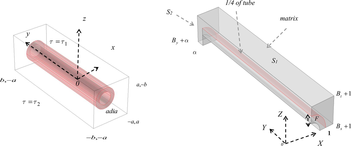
Elementary cell model of composite: perpendicular model.
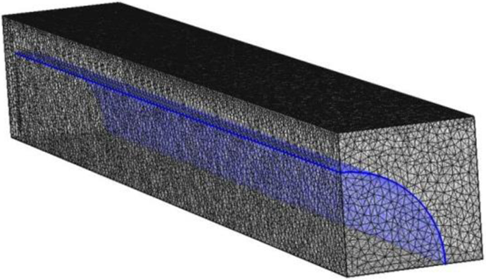
Mesh of the composite elementary cell, F = 1. F: dimensionless wall thickness of the hollow conductive tube.
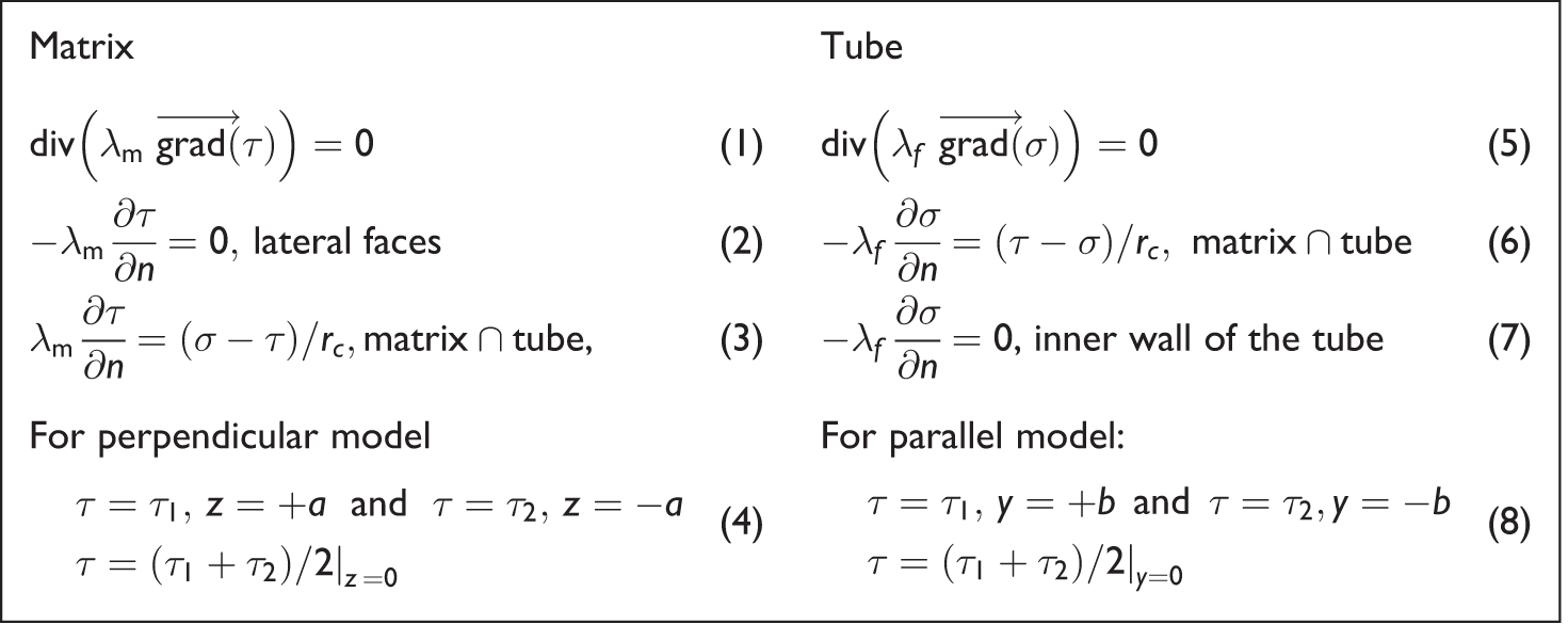
Where n is the normal unit vector pointing from the tube to the matrix, a is the half larger elementary cell (m), b is the half height of elementary cell (m), r c is the contact resistance, cube radius (m), τ 1 is the upper cell face temperature (K), and τ 2 is the lower cell face temperature (K).
To simplify the problem and to decrease the computing time, dimensionless parameters, and variables were used:


The ETC
Perpendicular ETC (Figure 1):
The heat flux crossing the elementary cell is defined by: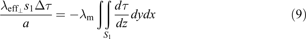
Introducing the lower cell face temperature and the dimensionless parameters, equation (10) can be re-written:
Thus we obtain the perpendicular ETC: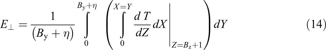
The heat flux (Q) in the Z-direction over the upper face (S
1) of the elementary cell is defined by: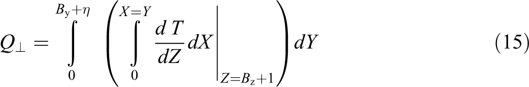
The perpendicular ETC and the filler volume fraction of the perpendicular model are given by:
Parallel ETC.
In the same procedure, we calculate the parallel ETC: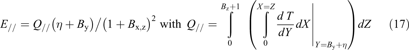
Analytical models
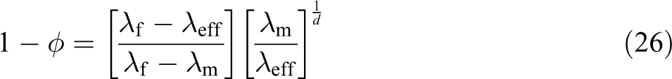
Many analytical models were proposed in the past to predict thermal conductivity of composite materials. However, only few models take into account the fillers size and the thermal contact resistance between fillers and matrix. Hasselman and Johnson
48
have proposed a modification of the Hashin and Shtrikman model
49,50
to take into account these parameters and applied this model to the study of dispersions of Nickel particles into a sodium borosilicate matrix. According to this model, also used by Benveniste,
12
the ETC λ
eff of composites materials is defined by: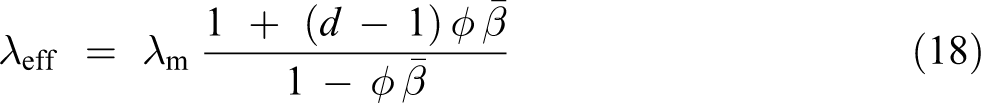
with
where ϕ is the filler volume fraction, λ
f is the filler thermal conductivity, λ
m is the matrix thermal conductivity, d is a parameter depending on the particle shape (d = 3 for spheres and d = 2 for cylinders), r is the radius of particles, and h
c is the contact conductance between the particle and the matrix and is defined by 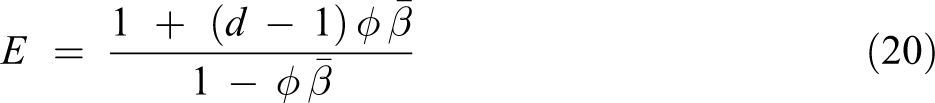
with
The model of Lewis & Nielsen is a model originally used for the prediction of mechanical properties of composites.
51
This model was also applied to the prediction of the ETC of composites
51
by taking into account different parameters for the prediction of ETC such as the shape, distribution and orientation of fillers into the matrix and also the thermal conductivity values of filler and matrix. The main interest for the use of such a model is that predictions also consider the value of the maximum packing fraction of fillers 
with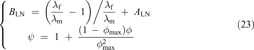
where 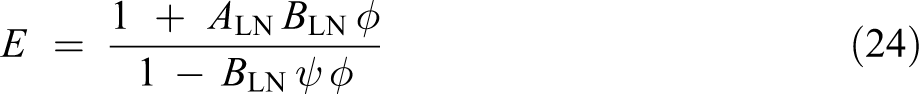
with: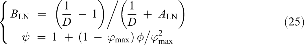
Unlike the Maxwell formula, the model proposed by Bruggeman takes care of the shape factor of the second-phase inhomogeneities. 52 Moreover, it has been argued that this model can be used to estimate the ETC with both low- and high-volume fraction of particles.
d = 2 for cylinders oriented perpendicular to heat flow and
For spherical inclusion, d = 3, and the ETC is defined by the following equation: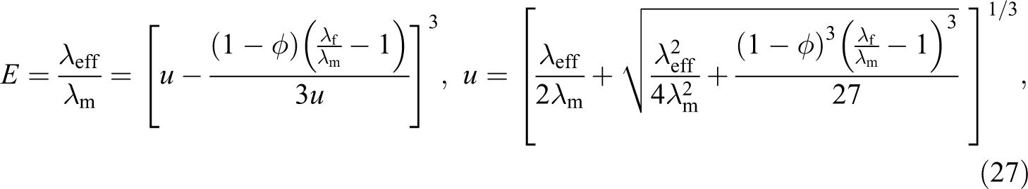
The Hatta and Taya model
53
describes an ETC

where: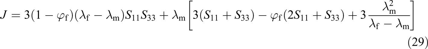
Experimental study
Sample preparation (epoxy resin/metallic hollow tube)
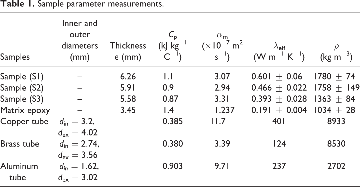
In our experimental setup, the matrix material is an epoxy resin of Vantico AG (Switzerland). The Araldite® LY5052 is mixed to 42% weight of Aradur 5052. This resin with a low viscosity (0.8 Pa s at 23°C) is then placed under vacuum for about 50 min to remove the air bubbles before injection. The metallic hollow tubes (Goodfellow, UK) are placed in a mold (200 × 200 mm2) with an equidistant distribution of 1 mm between the tubes (Figure 3 (a) to (c)). To facilitate the release of the resin, a Teflon film polytetrafluoroethylene (PTFE) was stacked on the mold surface. Once the mold was closed and sealed, the resin is introduced from the injection gate at ambient temperature and under constant pressure. Besides, the sample is pressurized in the mold, and the injection of an excess of material will be introduced to compensate the shrinkage. After reticulation of the injected resin, the mold and PTFE film were removed. Three configurations of samples were prepared under the same manufacturing conditions (S1, S2, and S3). The first, resin/hollow copper tube (99.9% copper (Cu)) with internal and external diameter of 3.2 and 4.02 mm, respectively. The second resin/hollow brass tube (70% Cu, 30% zinc) with 2.74 and 3.56 mm of internal and external diameter, respectively. The third one is resin/hollow Al tube composite (99.5% Al) with 1.62 and 3.02 mm of internal and external diameter, respectively (Figure 3). Thermophysical properties of the tubes are presented in Table 1.
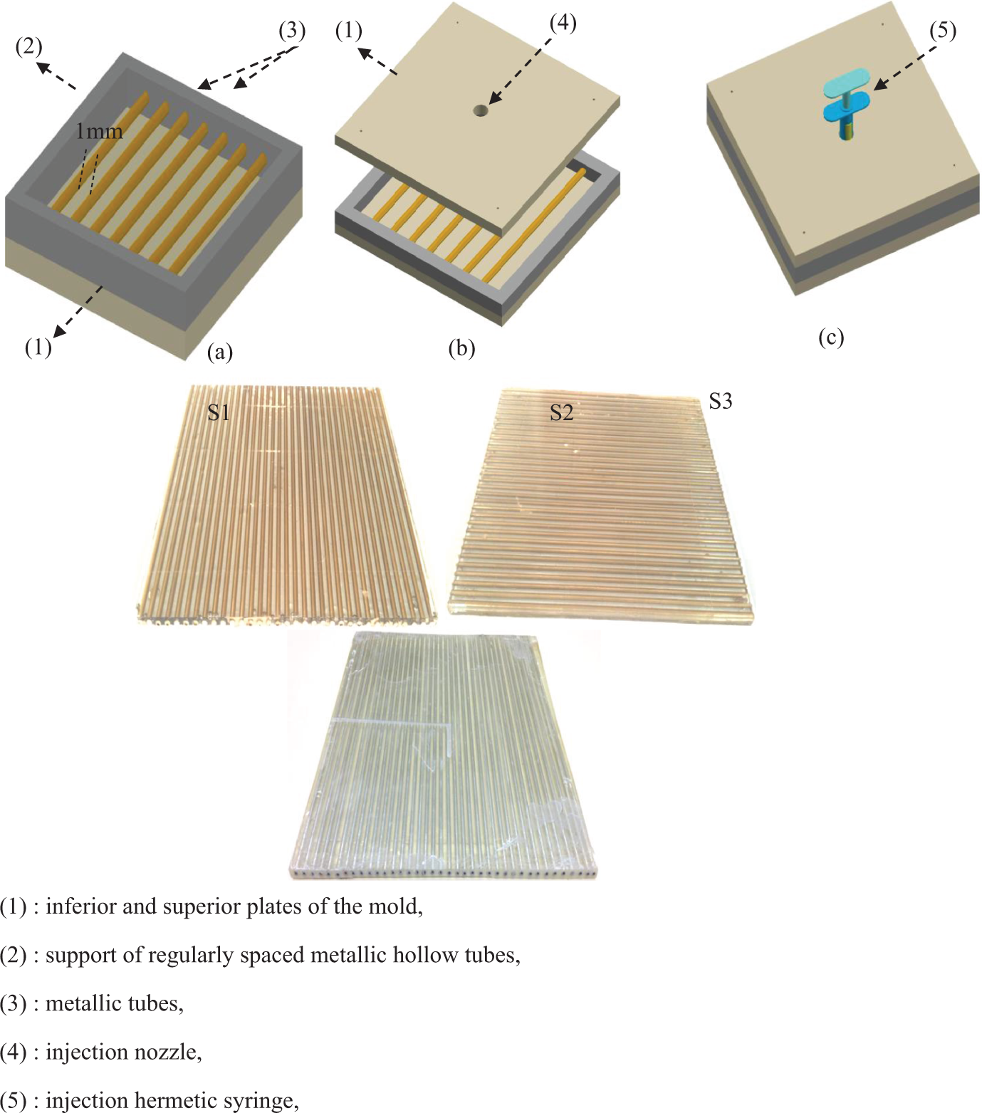
Manufacturing of epoxy resin/metallic hollow tubes composites. (a and b) Positions of metallic tubes into a mold and (c) process of injection. (S1) epoxy resin + copper tubes, (S2) epoxy resin + brass tubes, and (S3) epoxy resin + aluminum tubes.
Sample parameter measurements.
Thermophysical properties measurements
For large size samples, testing using a noninvasive method for thermophysical properties determination is necessary. The proposed test bench for the parallelepiped-shape of composite provides temperature and heat flux measurements at the material borders (see Figure 4). The sample is located between two horizontal heat exchanger plates of Al connected to thermoregulated baths that allow for the fine regulation of the temperature of the injected oil H10 with a precision of approximately 0.1°C. Heat flux sensors and thermocouples (types T and K) are placed on each side of the composite sample to measure the heat flux
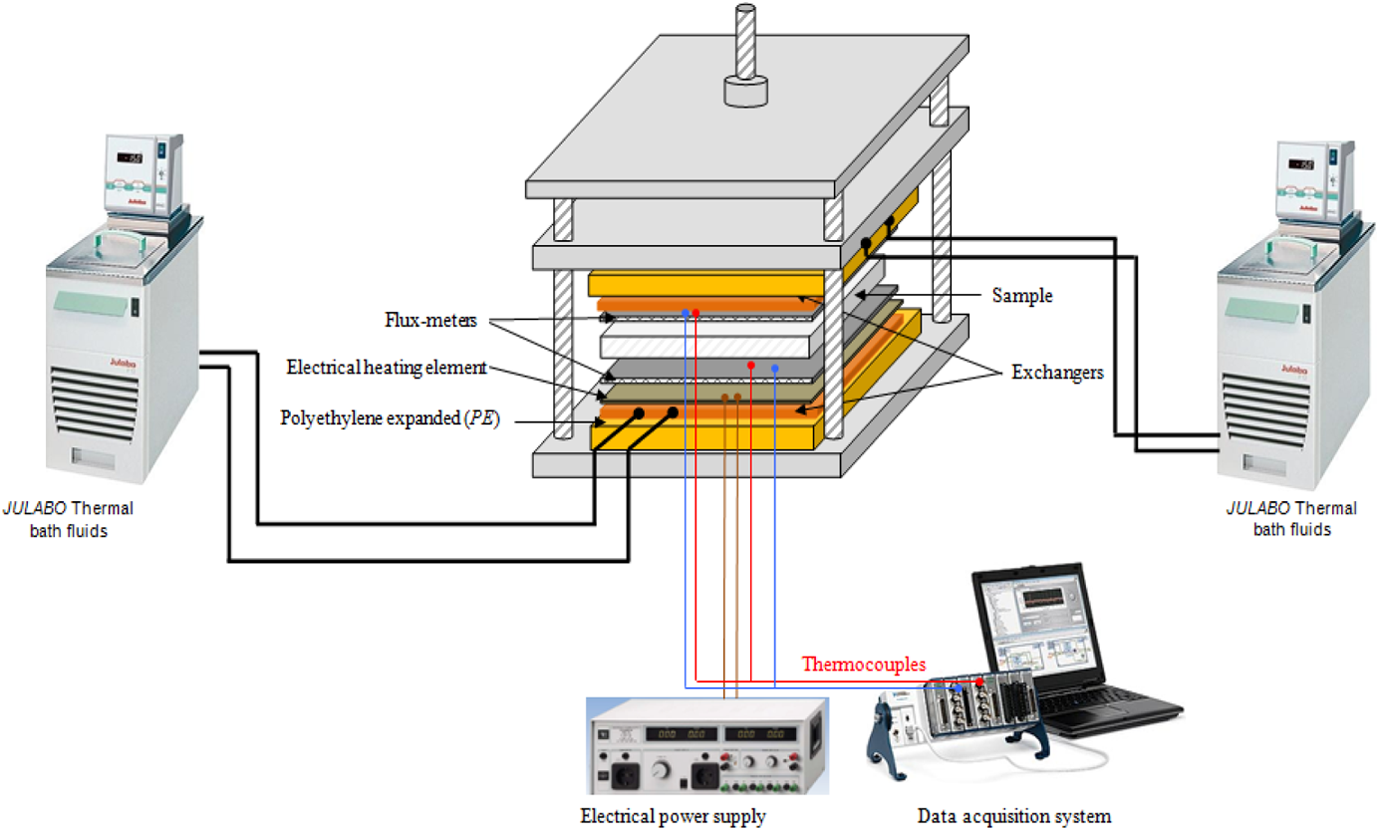
Experimental setup.
Results and discussion
Effect of filler volume fraction, thermal resistance, and D(F = 1)
In our previous study, the ETC for three elementary cells, such as simple cubic (SC), body-centered cubic (BCC), and face-centered cubic (FCC), were numerically and experimentally investigated.
36
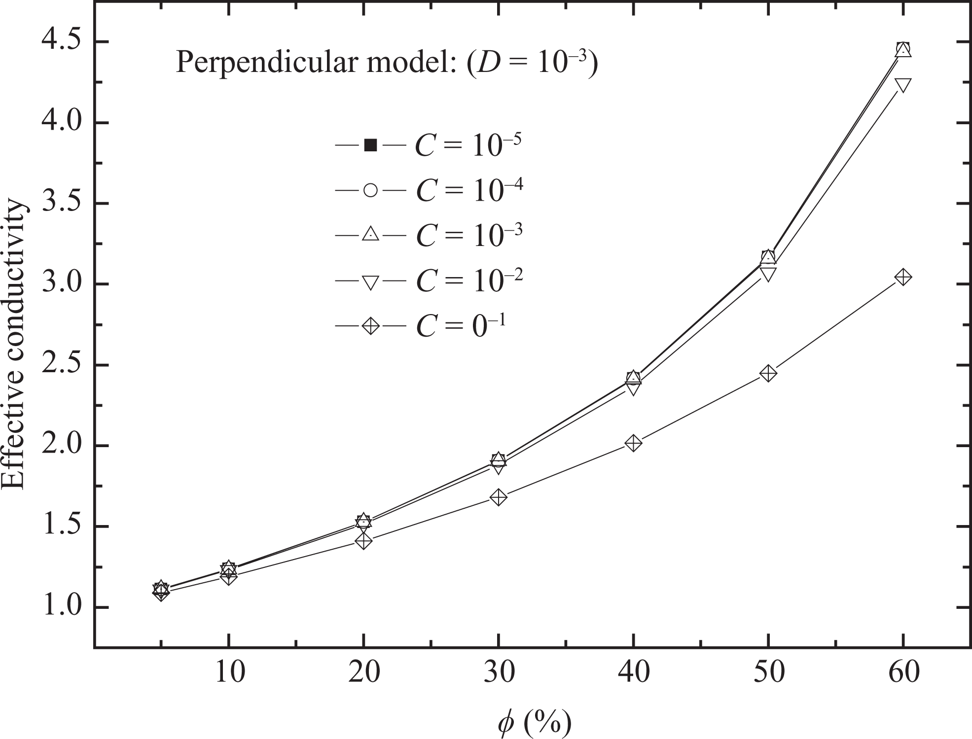
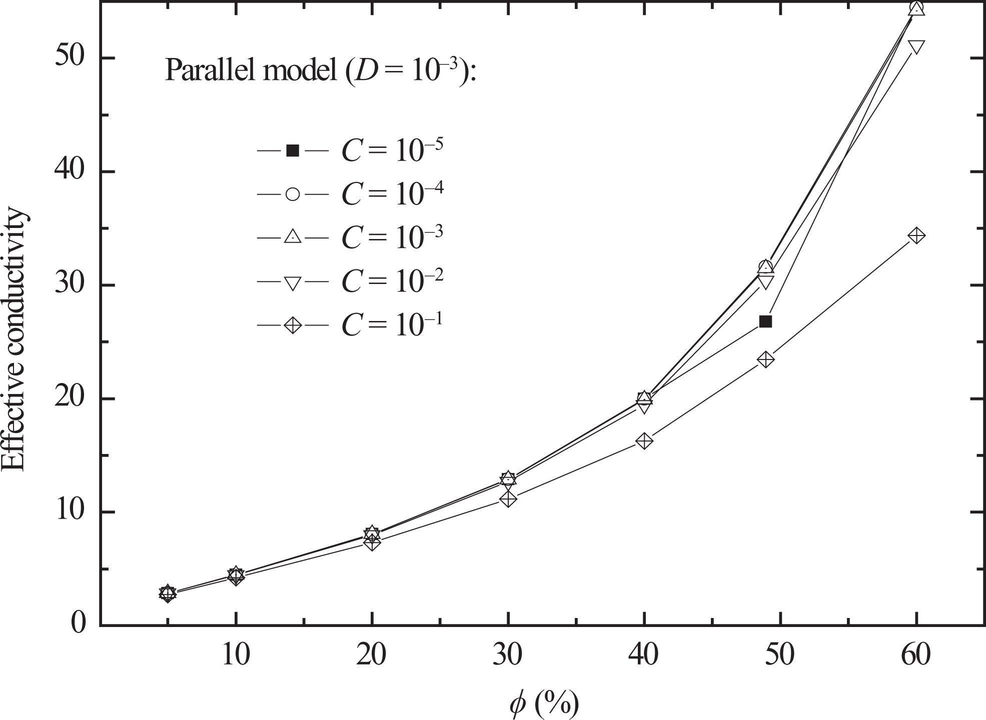
The focus of this section is on two-phase composites material filled with solid tube (F = 1). In Figures 5 and 6, the effect of the ratio of thermal conductivities of filler to matrix material and the Kapitza resistance of the contact inclusion/matrix was investigated for perpendicular and parallel tube composites. Computation of about 150E values has showed that a decrease in the contact resistance r
c or of the inner resistance
Perpendicular effective thermal conductivity.
Parallel effective thermal conductivity,
Perpendicular effective thermal conductivity,
Parallel effective thermal conductivity,
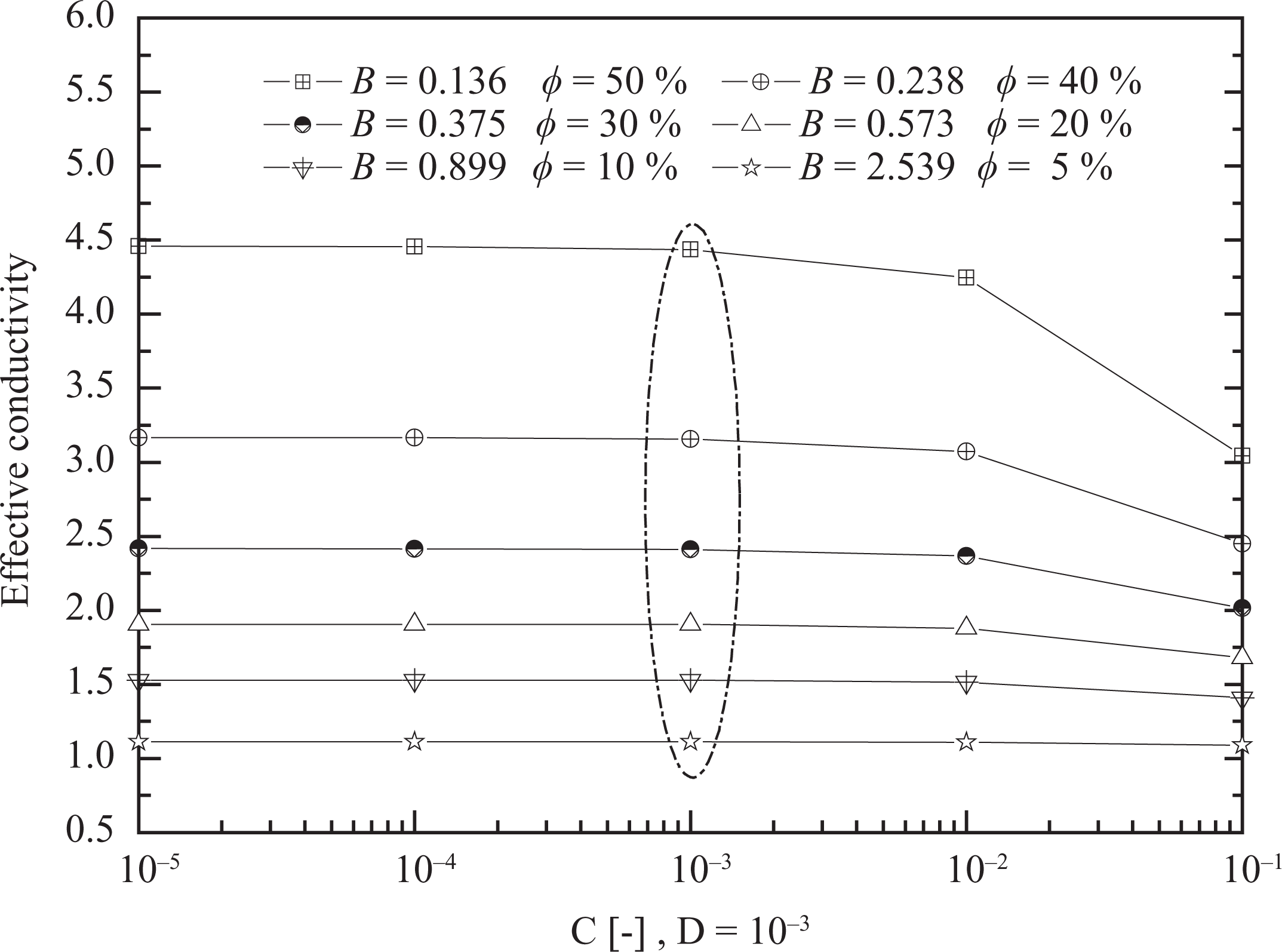
Perpendicular effective thermal conductivity, F = 1. F: dimensionless wall thickness of the hollow conductive tube.
Effect of the wall thickness of hollow tube,
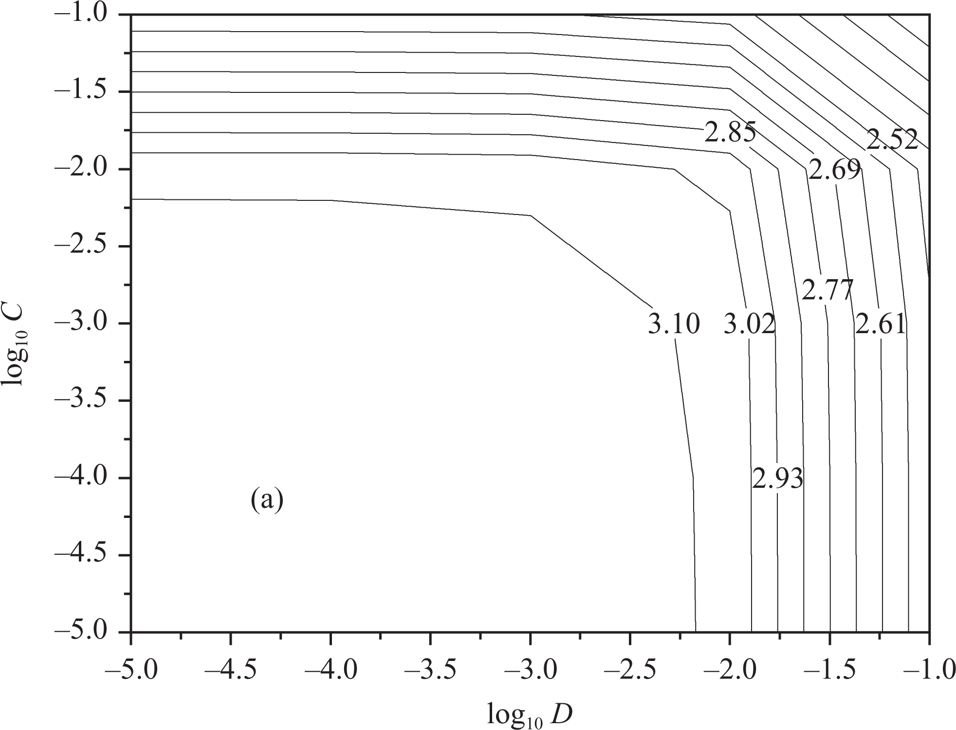
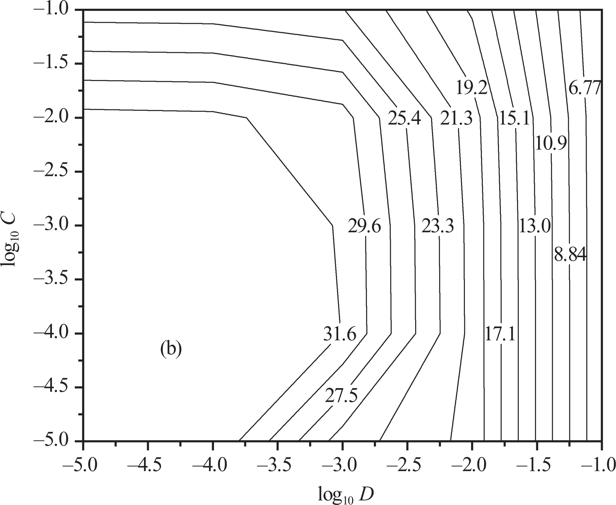
In this section, we will present numerical results obtained by using the proposed mathematical model to examine the contribution of the various factors affecting heat transfer in hollow tube/polymer composites and their effect on the overall effective thermal properties. First, we consider the effect of tube wall thickness on the effective conductivity at constant thermal contact resistance C and inner resistance D. Figure 10(a) and (b) show the numerical results for D = 10−3 and C = 10−5 for perpendicular and parallel models, respectively. The wall thickness varies from 0.05 to 1. Figure 10(a) shows the evolution of the
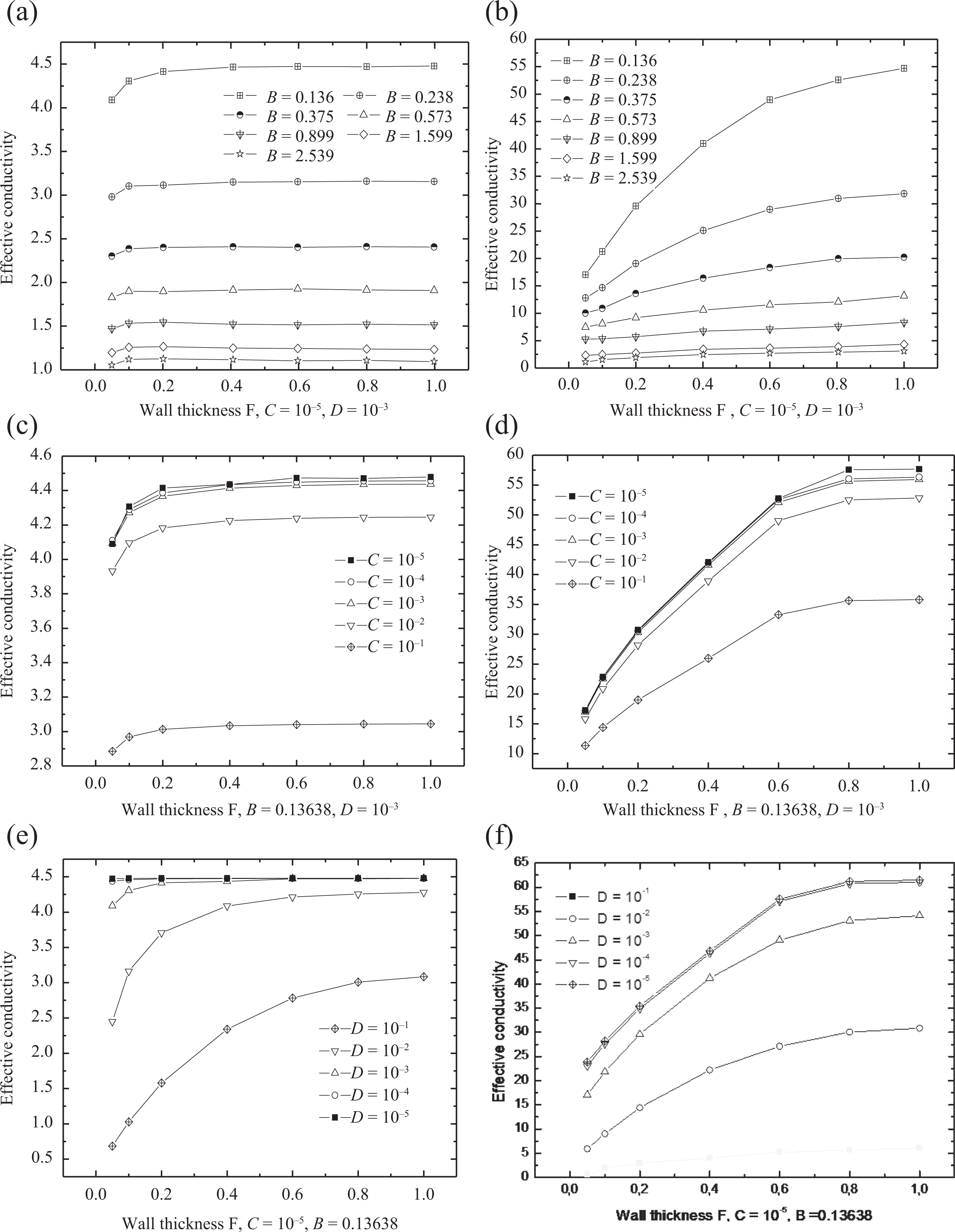
Effective thermal conductivities
Second, we examine the influence of the reduced contact resistance on the effective conductivity. The variation of the effective conductivity with the increase in C is shown in Figure 10 (c) and (d) for perpendicular and parallel models, respectively. However, it can be seen that the effective conductivity increases with the decrease in the interfacial contact resistance C. At low values of the thermal contact resistance
Comparison between analytical models and numerical simulations
The effective conductivity of parallel reinforcement composite has been calculated using the proposed numerical model. A comparison has been made with the predictions of standard models like those of the Bruggeman,
52
Hashin and Shtrikman,
50
Hatta and Taya,
53
and Lewis-Nielsen.
51
The choice of these models was based on two reasons: the model of Hashin and Shtrikman is one of the bases of many recent thermal conductivity models, and the model of Hatta and Taya, among the models developed recently, provides good agreement between the calculated values and the numerical data. Figure 11 shows a comparison between theoretical models and numerical simulations. As seen in this figure, the ETC values
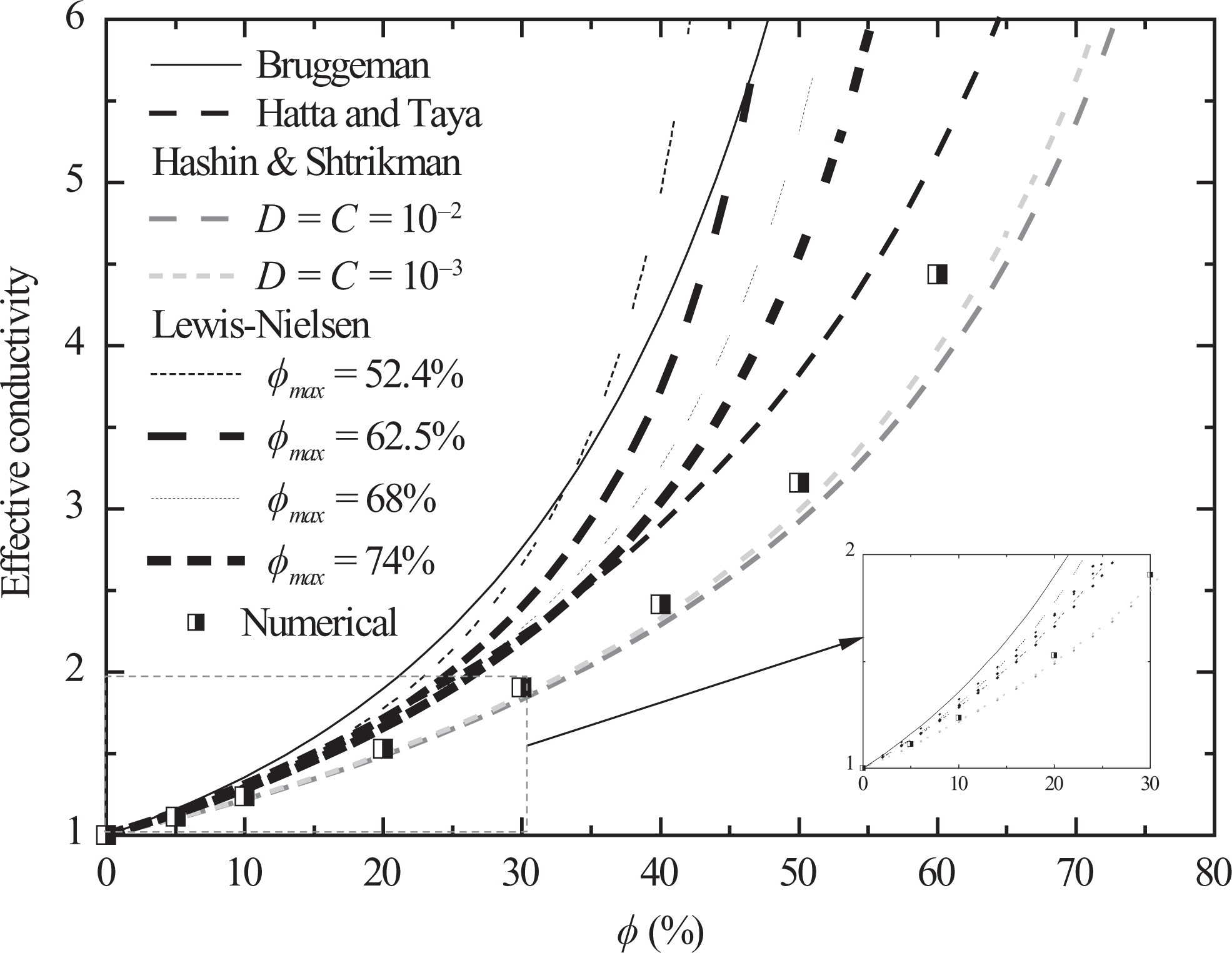
Comparison between analytical models and the calculated effective thermal conductivity
ETC and heat capacity measurements
To experimentally determine thermal apparent conductivities of the hollow tube composites, a temperature difference was imposed between up (T
1) and down (T
2) sides of the samples until observing a zero heat flux (equilibrium state q
1 = q2). First, the temperature levels on both sides (T
1 and T
2) are fixed and maintained until thermal equilibrium. At time t = 0 h (Figure 12), the composite was heated by modifying the temperature on a single face only (T
1 > T
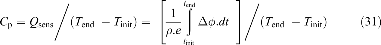
2) until obtaining a thermal steady state. A similar experiment was carried out for all samples; the material is subjected to a temperature difference. Several tests were carried out on the material to check the reproducibility of the measurement. The apparent thermal conductivities are calculated using equation (30). To measure heat capacity of the samples,
54
the experiment consists first in imposing on the sample a superficial temperature of
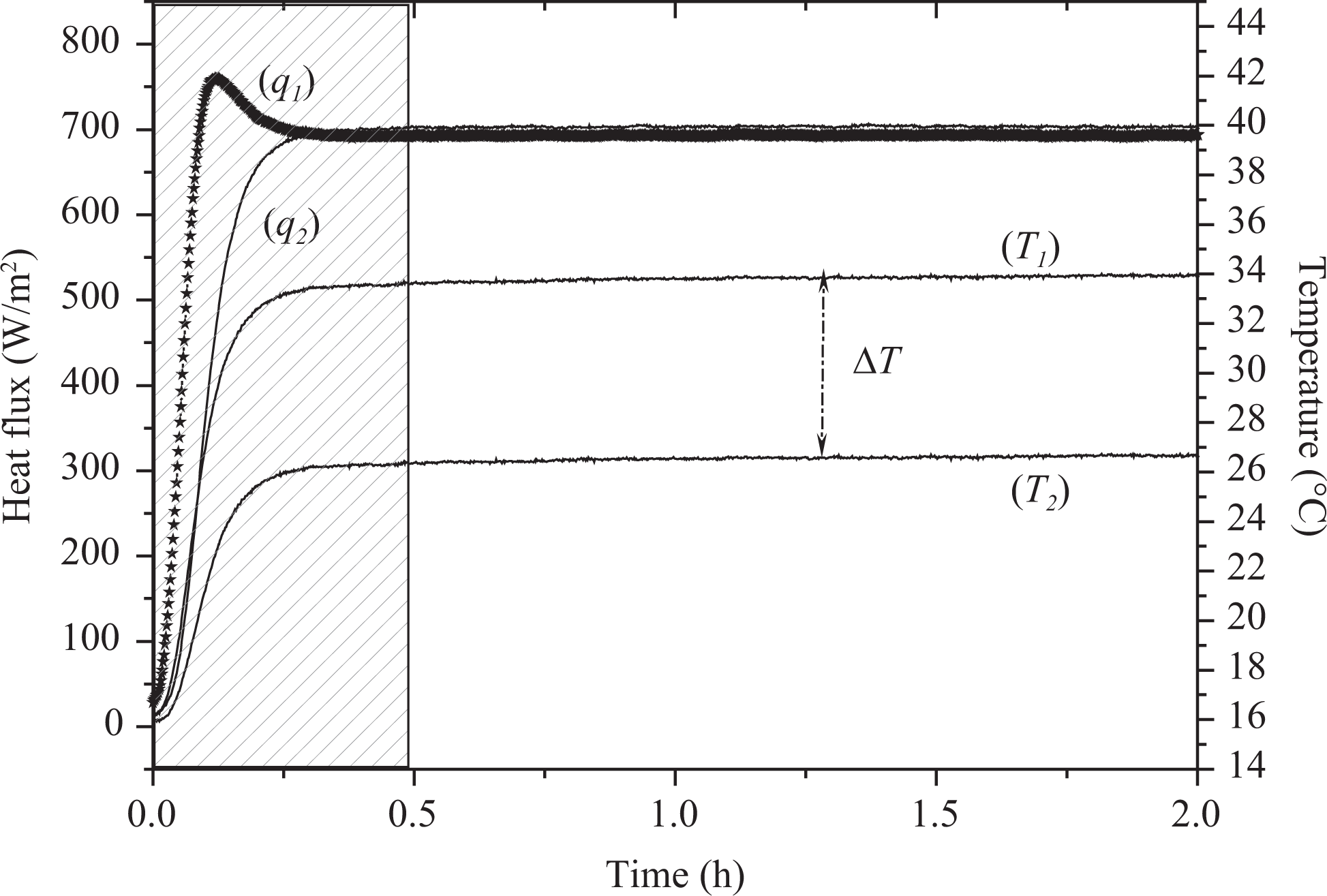
Determination of thermal apparent conductivities of the composites (S1). S1: sample 1.
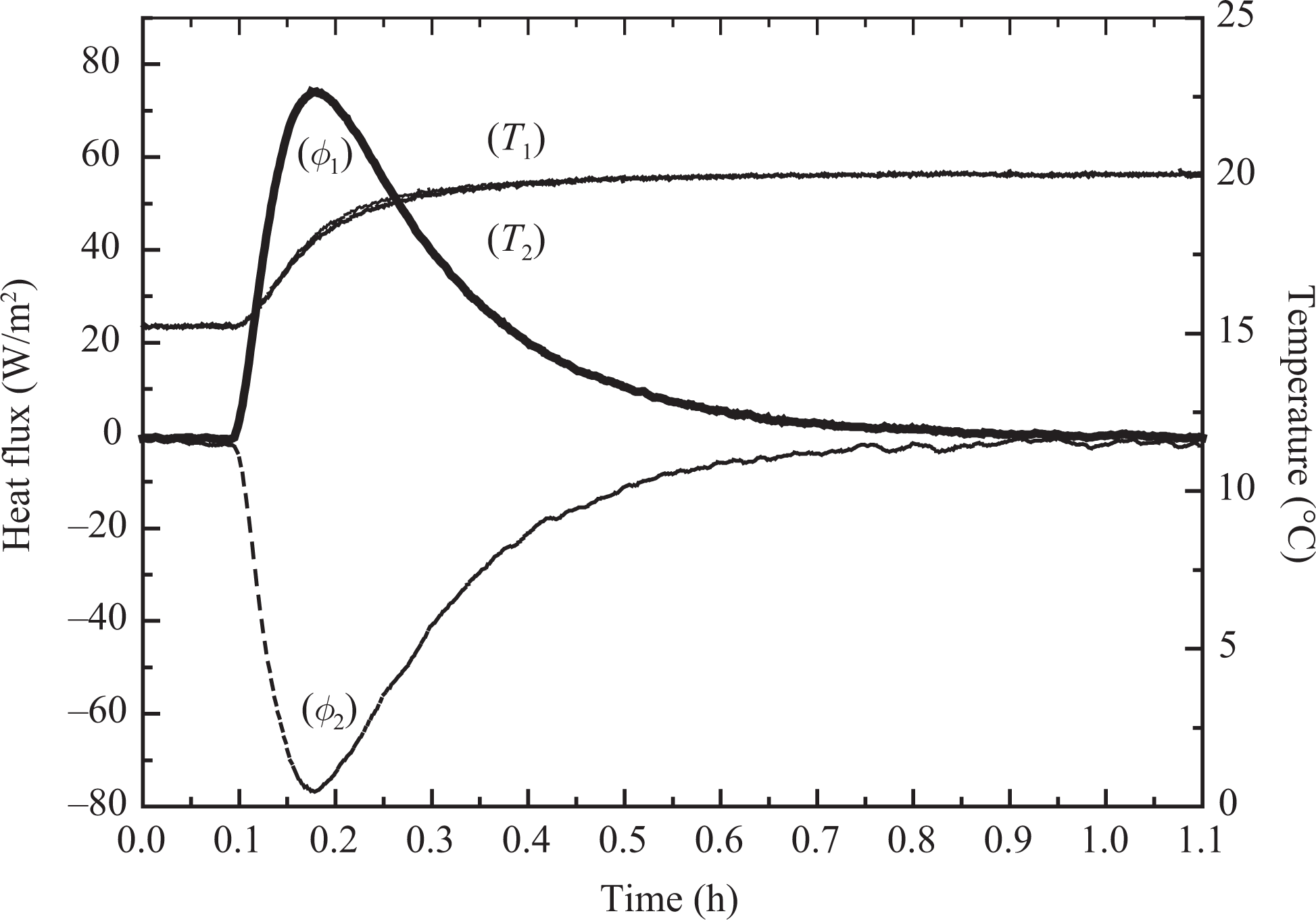
Heat flux and temperatures evolution of S1 (15°C to 20°C). S1: sample 1.
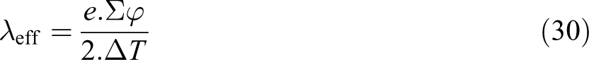
Where e is the thickness of the sample;
Comparisons between simulations and experimental data
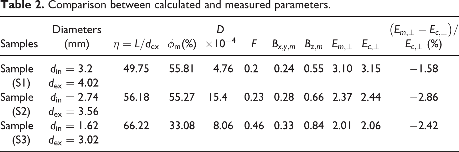
To illustrate the difference between the measured effective conductivities and the calculated values from FEM simulations, we have considered that the contact resistance is lower between the hollow tube and the epoxy matrix (C = 10−5). The choice of this value is inspired from Chapelle’s
55
study. His work is focused on the characterization of the interfacial thermal resistance between metallic wires and a polymer matrix and has found values between 3E−6 m2 K−1 m−1 and 1.7E-5 m2 K−1 m−1. Table 2 shows the experimental values
Comparison between calculated and measured parameters.
Conclusion
In this article, we have presented a mathematical model for calculating the ETC of hollow tube/resin composite. We have shown here, numerically, that the ETC will be calculated using a representative volume element based on the finite element software COMSOLTM version 4.2a. It has also been shown that the interfacial resistance significantly affects the overall ETC. It was also found that the effective conductivity is especially sensitive to the parameter F and higher in the parallel model. This parallel thermal conductivity is increasing by up to 157% by raising the wall thickness from 0.05 to 1 (Figure 10(d); C = 10−5). Based on the results (Figure 10 (a), (c), and (e)), wall thickness does not strongly affect the perpendicular ETC. The rise in
Footnotes
Declaration of Conflicting Interests
The author(s) declared no potential conflicts of interest with respect to the research, authorship, and/or publication of this article.
Funding
The author(s) received no financial support for the research, authorship, and/or publication of this article.