
Abstract
In-plane prebuckling stresses arise under axial edge loading as a result of a plate boundary being restrained from deformation in the plane of the plate. These stresses exhibit a uniform distribution only under a special set of boundary conditions and in general such uniform in-plane stress distributions do not exist under most boundary conditions encountered in practice. In the present study, in-plane prebuckling stresses are investigated for various in-plane boundary constraints and the stress contour lines are given for rectangular cross-ply laminated plates under linearly varying edge loads. The second part of the article involves the computation of the optimal layer thickness to maximize the buckling load under various combinations of in-plane boundary restraints. The numerical solutions are obtained by finite elements based on first-order shear deformable plate theory which include the in-plane deformations as nodal degrees of freedom. Numerical results show that the exclusion of the in-plane restraints may lead to errors in stability calculations and consequently in the design of laminated plates.
Introduction
In this study, the influence of in-plane boundary restraints on in-plane stresses and the buckling of rectangular cross-ply laminates are investigated under linearly varying compressive edge loads. It is observed that presence of in-plane restraints on the deformation of a plate leads to nonuniform distribution of in-plane stresses which in turn affect the buckling load.
The effect of various in-plane boundary restraints on buckling of plates has been investigated by Harris, 1 Sherbourne and Pandey, 2 Bedair,3,4 and Nemeth. 5 Such restraints are known to lead to thermal buckling as studied by Nemeth6,7 and Jones. 8 These boundary conditions arise in many applications and lead to a nonuniform distribution of in-plane stresses which require a numerical approach for their study. Such stresses, for example, arise in the web sections of transversely loaded composite beams and may lead to premature failure if not taken into account in the design phase. Restraints against in-plane movement typically also arise in aerospace structures where adjacent panels and stiffeners cause these constraints. 5
Another complicating factor arises when the plate is subjected to linearly varying in-plane loads leading to buckling. In this case, prebuckling deformations have to be taken into account in the computation of the buckling load.9–11 This problem has been studied by Papazoglou et al., 12 Nemeth,13–15 Zureick and Shih, 16 Leissa and Kang, 17 Kang and Leissa, 18 Wang et al., 19 and Zhong and Gu.20,21 Papazoglou et al. 12 investigated the buckling of symmetric laminates under linearly varying in-plane loads using the Rayleigh-Ritz method based on classical lamination theory. The infinitely long laminates under linearly varying axial loads were studied by Nemeth.14,15 Leissa and Kang 17 obtained exact solutions for the free vibration and buckling of rectangular plates subjected to a linearly varying compressive load with two opposite edges simply supported (SS) and the other two edges clamped (C). They extended these results to other boundary conditions as reported elsewhere. 18 Wang et al. 19 employed a differential quadrature method to study the vibration and buckling of an SS-C-SS-C plate subject to linearly varying in-plane loads. The effect of various in-plane boundary restraints on the optimization of laminates under linearly varying buckling loads has been studied by Adali and Cagdas. 22 Experimental results on the buckling of anisotropic laminates under linearly varying loads were discussed by Romeo and Ferrero. 23 Apart from the linearly varying in-plane loads, buckling of laminates under other nonuniform edge loads have been investigated by Kam and Chu, 24 Bert and Devarakonda, 25 Devarakonda and Bert, 26 Jana and Bhaskar, 27 Wang et al.,28,29 and under in-plane moments by Kang and Leissa. 30 Devarakonda and Bert 26 explained the stress diffusion phenomena and showed that under nonuniform in-plane loads, the membrane force distribution is not constant inside the plate, and presented explicit results for buckling loads in comparison with numerical results obtained using finite element method (FEM).
In many of the previous studies stated above, the buckling loads were calculated assuming the stress distribution in the plate was constant and also the in-plane boundary conditions were not fully described. 2 The boundaries were generally defined as either SS or C; however, specifying the in-plane boundary conditions often models a structure more precisely. For example, stiffeners also change the stress distribution considerably in the plates as shown by El-Ghazaly et al. 31 In this study, only the effect of in-plane/membrane boundary conditions was investigated and the in-plane stress distributions under external loads were calculated before performing a linearized stability analysis by FEM. It was observed that the exclusion of the in-plane restraints leads to errors in the stability calculations. Reasons for excluding in-plane boundary restraints in many studies include the facts that analytical solutions in the presence of in-plane boundary constraints do not exist or not accurate enough. Similarly, the use of finite elements which do not include the in-plane deformations as nodal degrees of freedom leads to inaccurate computations. To compare the present results with those available in the literature, the boundary conditions where the in-plane stress distribution can be taken as constant are also studied in the present work.
Buckling analysis of laminated composite plates using the first-order shear deformation plate theory (FSDT) was given by Khdeir and Librescu, 32 but this work was restricted to uniform loads. Zhong and Gu 20 developed an analytical solution for the buckling of SS rectangular Reissner–Mindlin plates subjected to linearly varying in-plane loading. Buckling loads obtained by the classical laminated plate theory can have significant errors increasing with an increase in the degree of anisotropy and thickness of the plate.32,33 Thus, finite element formulations based on classical theory are of limited use in the analysis of composite structures due to the transverse shear effects. 34 In view of this, in the present work the plate-finite element is based on the FSDT. Daripa and Singha 35 studied composite laminates under localized in-plane loads using shear deformable plate-finite elements.
The present work investigates the in-plane stress distribution of cross-ply laminates under linearly varying edge loads and in-plane boundary restraints using finite elements based on the FSDT. An outline of the finite element formulation and the description of the finite elements are discussed in the next section. Next, the finite element solution is applied to a number of verification problems to assess its accuracy. Subsequently the prebuckling stresses are studied under linearly varying edge loads. A related problem is the computation of the optimal layer thicknesses to maximize the buckling load. The results for the optimal design problem are given for linearly varying and uniform edge loads and the efficiencies of the designs are obtained.
Finite element formulation
Next, the formulation for the parabolic isoparametric plate element used in the calculations is discussed. One of the reasons for selecting the 8-noded elements is to avoid the parasitic shear or shear locking problem which arises when linear isoparametric elements are used. Using the curved elements and making use of reduced integration, the shear locking problem can be avoided. The second reason is the ease in modeling complex geometries. Note that, the finite element code used in this study is written in Matlab® environment.
First-order shear deformable plate theory
The displacement field corresponding to FSDT for composite laminated plates is as follows:
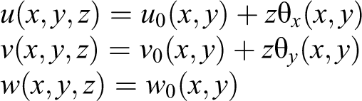
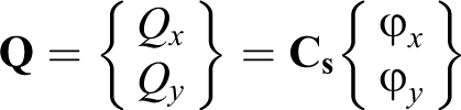
where u 0, v 0, and w 0 are the mid-surface displacement components and θ x , and θ y are the rotations of the transverse normal about the y and x axes. The x–y plane coincides with the mid-surface of the plate, with the plate thickness denoted by t. The strain–displacement relations are given by
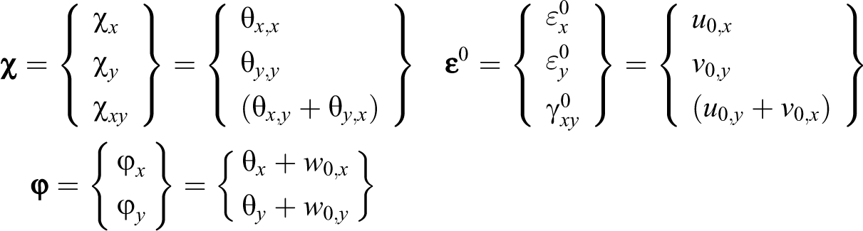
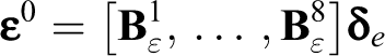
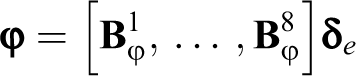
where φ
x
and φ
y
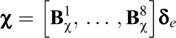
are the rotations due to shear about the y and x axes; and χ
x
, χ
y
, and χ
xy
and

Moments, normal forces, and shear forces are given in equations (3)–(5), as follows:
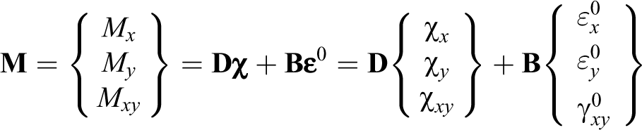
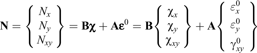
where for a laminated plate the matrices
Linear static analysis using FEM
The interpolation function of the displacement field is defined as follows:
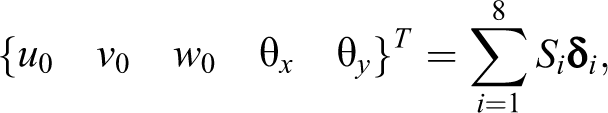
where Si
is the shape function at node i, and the displacement vector at node i is
where
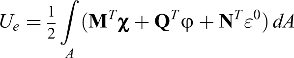
The total potential energy can be minimized by differentiating Ue
with respect to
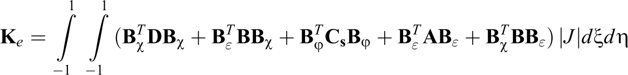
where |J| denotes the determinant of the Jacobian matrix and (ξ,η) denotes the coordinates of any point in the curvilinear coordinate system.
Linearized stability analysis using FEM
The steps of the solution can be briefly explained as follows 37 :
Calculate the membrane forces using a standard plane-stress analysis.
Calculate the initial stress or geometric stiffness matrix using the membrane stresses calculated in step (i).
Calculate the buckling load parameter λ, which is defined as the ratio of actual buckling load to the applied forces at which the plate buckles, by solving the eigenvalue problem which is solved using the Matlab® function as follows:
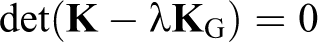
where
Element geometric stiffness matrix
The element geometric stiffness matrix is derived considering that the plate element is subjected to a prescribed in-plane stress system leading to buckling. The nonlinear terms of the mid-surface strains associated with the von Karman plate theory are given by Reddy 36
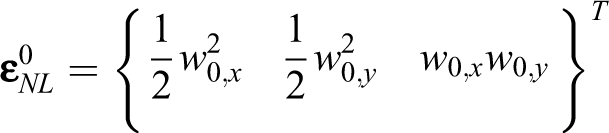
The potential energy of the applied stresses denoted by Ve arising from the action of the in-plane stresses on the corresponding second-order strains is given in
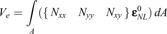
where Nxx , Nxy , and Nyy are the in-plane forces at the Gauss points which are calculated by a primary static analysis. For this purpose, a linear static analysis should be performed prior to linearized stability analysis. Thus, the calculation of the buckling load parameter involves two stages, the first stage being the linear static analysis and the second stage being the linearized stability analysis. Rewriting the terms inside the integral yields:

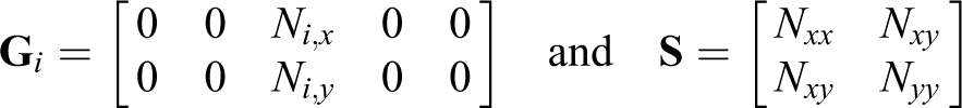
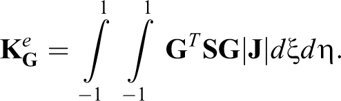
The element geometric stiffness matrix can be obtained by differentiating Ve
with respect to
Stress evaluation-smoothing technique
The Gauss points are the best points to calculate stresses; however, especially for comparison purposes, the stresses at the element nodes are also required. To solve this problem, a technique described by Barlow 38 and in Hinton and Owen, 39 which is a bilinear extrapolation of the 2 × 2 Gauss point stress values, is used.
Verification problems
Two verification problems are solved in order to validate the finite element code discussed in the section on finite element formulation.
Buckling of a rectangular plate subject to linearly varying loads
Stability analysis results for a SS homogeneous isotropic plate of dimensions a × b under the action of a linearly varying axial load are presented in comparison with the results presented by Timoshenko.
40
The geometry and loading details are shown in Figure 1 and the edge load, Nxx
, is defined in Eq. (18). The critical value of stress, σ
cr
, is defined as
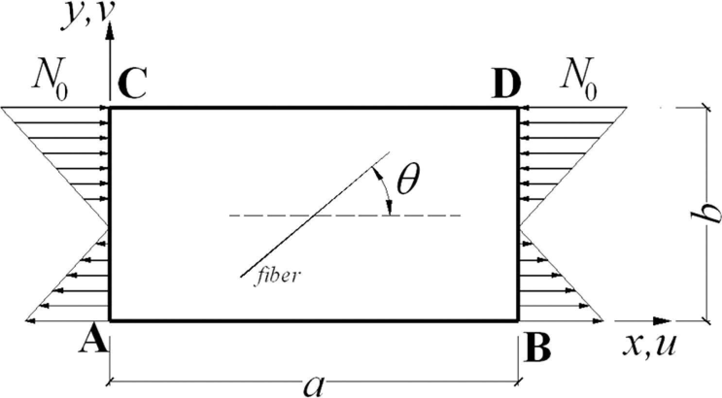
Plate geometry and linearly varying edge load.
As shown in Table 1, the numerical results obtained using a 16 × 8 finite element mesh are in good agreement with the reference results. However, the finite element results obtained are slightly lower than the results presented by Timoshenko 40 due to the influence of shear deformation taken into account here.
Numerical values of k in comparison with the analytical results with H/b = 0.01.
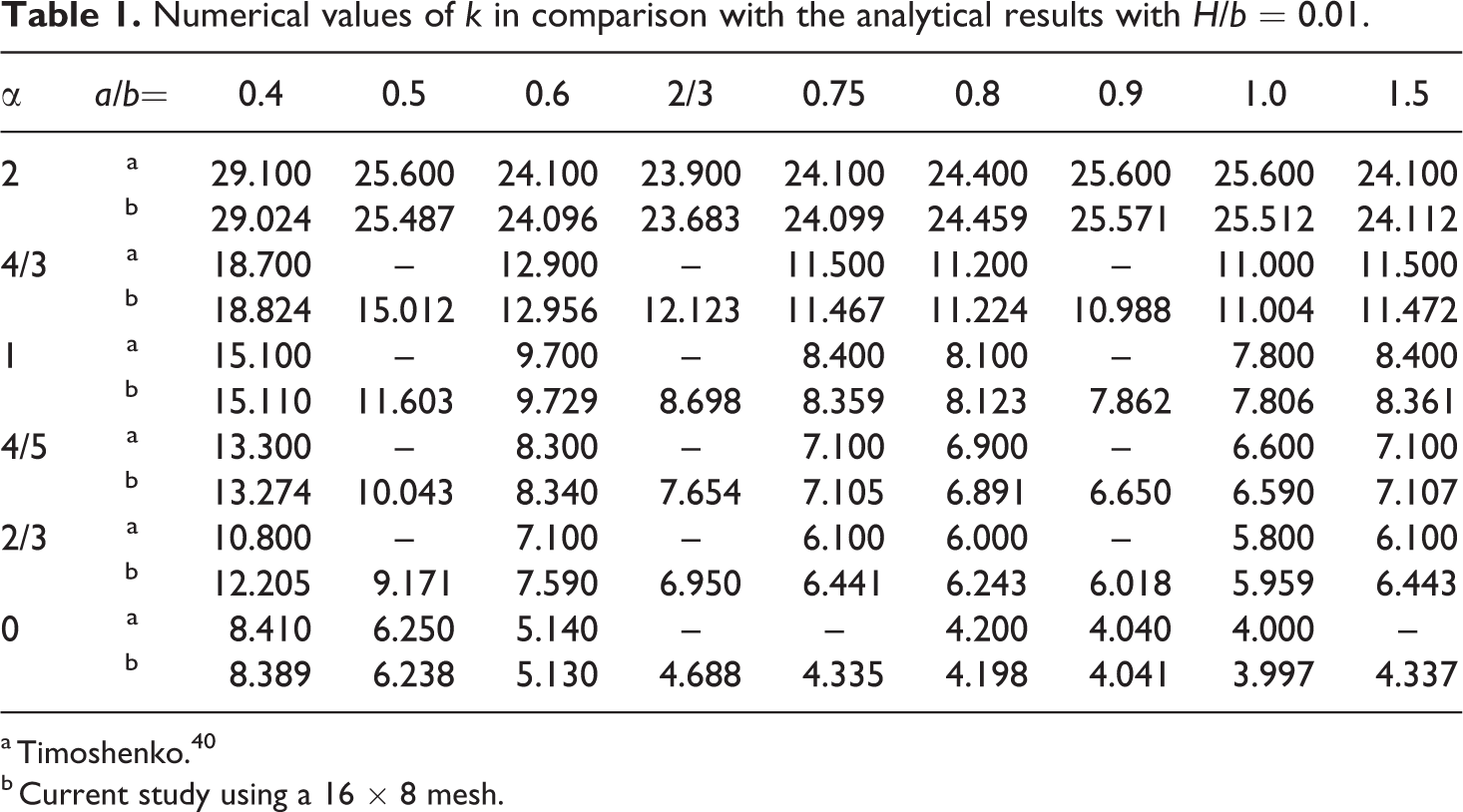
a Timoshenko. 40
b Current study using a 16 × 8 mesh.
Buckling of an antisymmetric cross-ply laminate under uniaxial compression
Stability analysis results for a SS rectangular antisymmetric cross-ply laminated plate subject to a uniform axial compression are presented in comparison with the results presented by Reddy and Miravete. 41 The lamina thicknesses are equal and the material properties are taken as
E 1 /E 2 = 25, ν 12 = 0.25, G 12 /E 2 = G 13 /E 2 = 0.6, G 23/E 2 = 0.25.
The results obtained are tabulated in Table 2, in comparison with the reference results, where the abbreviations 2Q8R, 2Q9R, and CFS stand for 8 node finite elements with reduced integration, 9 node finite elements with reduced integration, and closed form solution, respectively. The plate is modeled using a 16 × 8 regular mesh. The nondimensional buckling load,
Nondimensional buckling loads for antisymmetric cross-ply laminated plates under uniaxial compression, a/H = 10
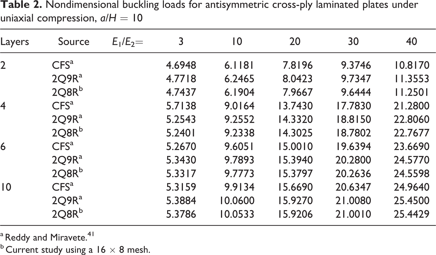
a Reddy and Miravete. 41
b Current study using a 16 × 8 mesh.
Problem definition
A rectangular plate of lateral dimensions a × b and thickness H is subjected to a linearly varying compressive edge loading as shown in Figure 1. Nxx , Nyy , and Nxy are normal forces per unit length in the x and y directions and shearing force per unit length in the xy plane, respectively. The in-plane edge forces Nxx , Nyy , and Nxy along the edges x = 0 and x = a are given in Eq. (18) with the other edges being stress free, as follows:
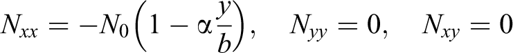
where N 0 is the intensity of Nxx at the edge y = 0 and α is a constant. By changing α, we can obtain different load cases, that is, α = 2, α < 2, and α > 2 corresponds to pure bending, a combination of bending and compression, and a combination of bending and tension, respectively. For all values of α, Nxx = N 0 at y = 0. In particular, Nxx = 0 at y = b for α = 1, Nxx = 0 at y = b/2 and Nxx = −N 0 at y = b for α = 2 which are the α values used in the numerical study of the problem with the case α = 0 corresponding to the uniform compression. The nondimensional buckling load parameter, λ, is defined as
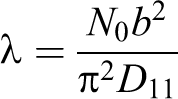
where D
11 denotes the flexural rigidity of the plate defined by
The entries of
Boundary conditions
The four different sets of boundary conditions are tabulated in Table 3 and schematically shown in Figure 2, where the sides AC and BD refer to x = 0 and x = a, respectively, and the sides AB and CD refer to y = 0 and y = b, respectively, as shown in Figure 1. Rotational restraints are the same for SS-I and SS-II boundaries and for C-I and C-II boundaries, the only differences being the in-plane boundary conditions. The boundary sets SS-I and SS-II are grouped as the SS plates and the boundary sets C-I and C-II are grouped as the C plates.
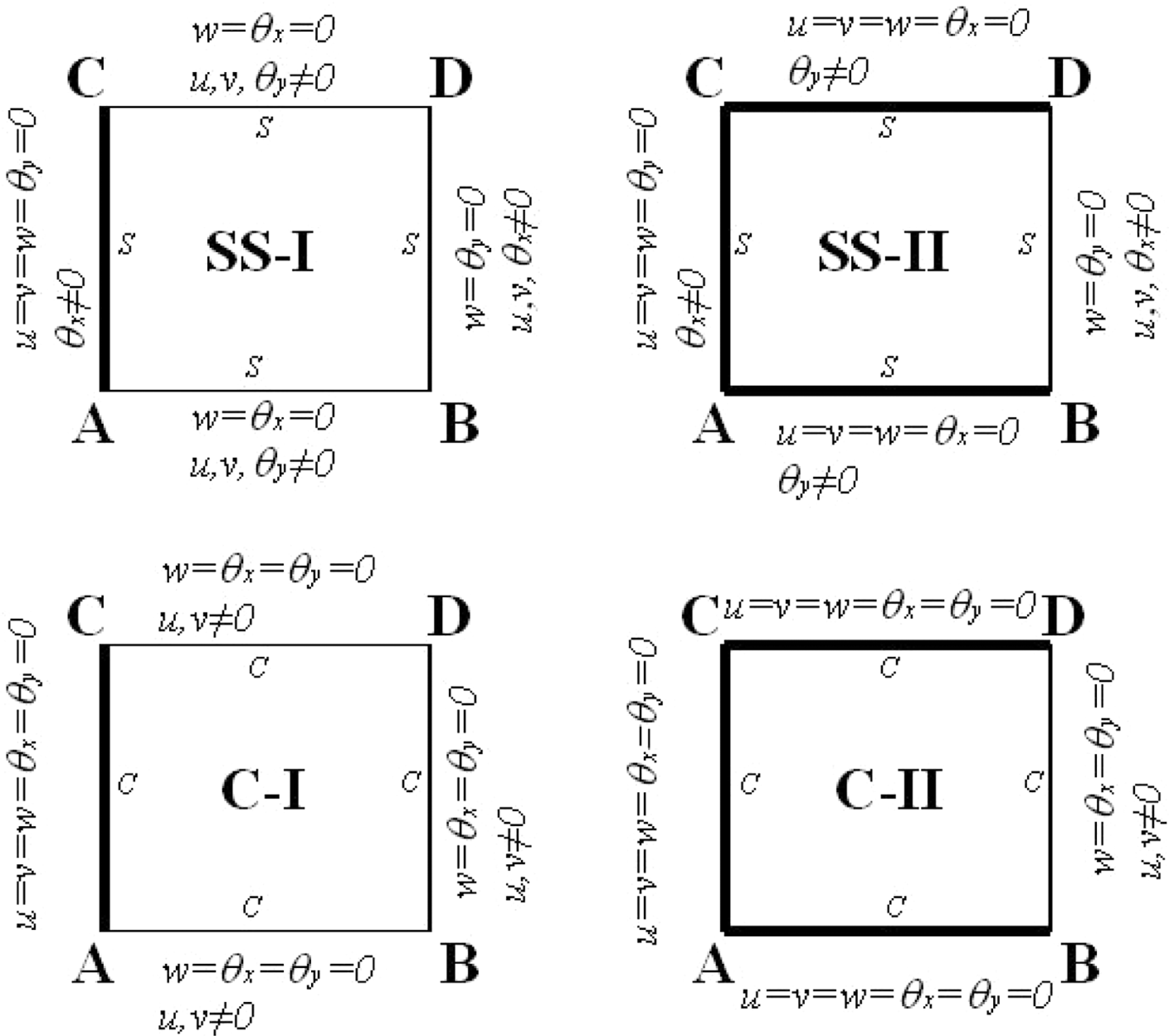
Schematic representation of the boundary conditions simply supported (SS)-I, SS-II, clamped (C)-I, and C-II edges.
Boundary conditions; 1: free, 0: restrained
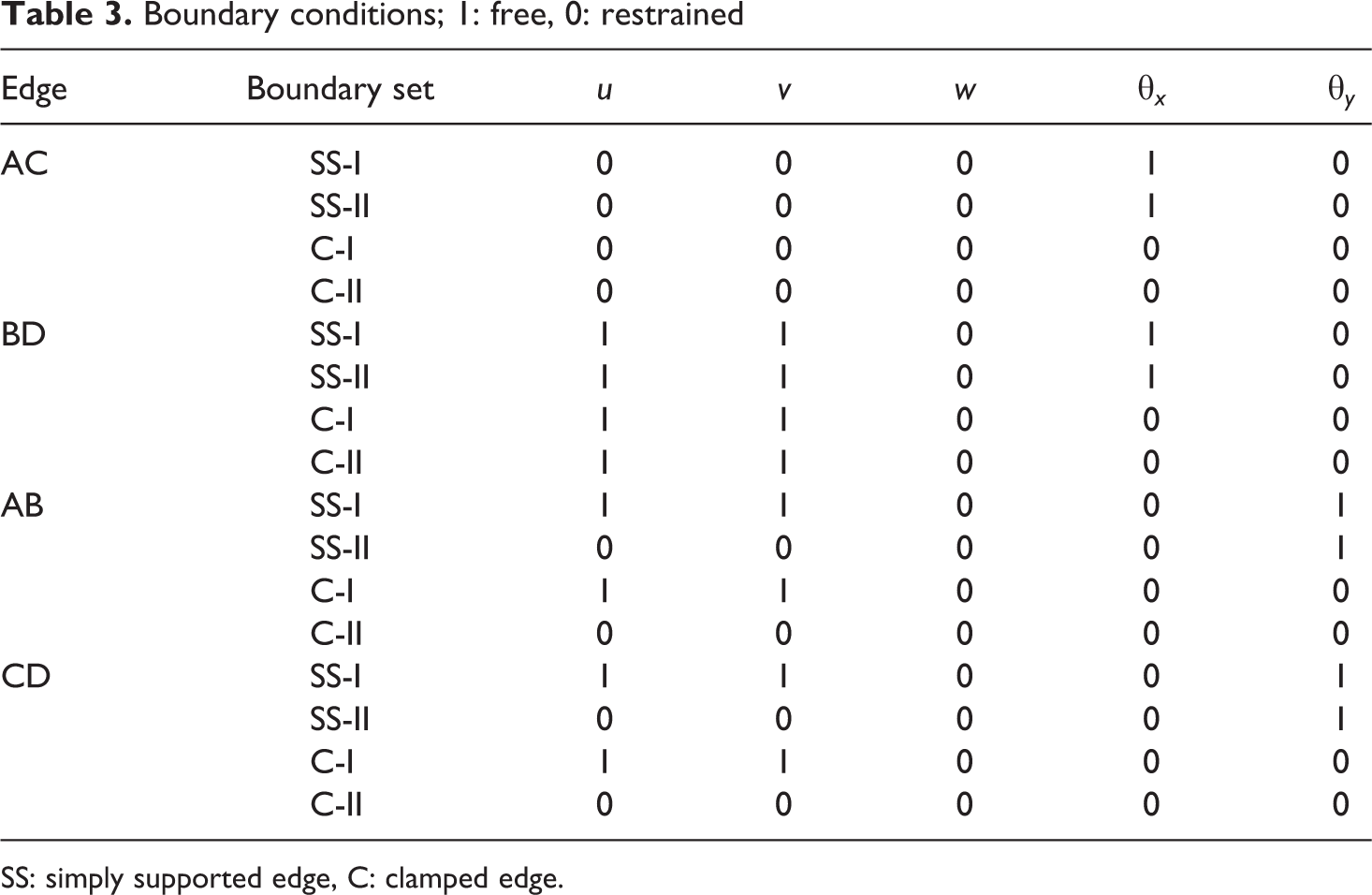
SS: simply supported edge, C: clamped edge.
Design problem
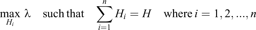
The design objective is to maximize the nondimensional buckling load of the symmetrically laminated rectangular plate of total thickness H, total layer number n by optimizing the ply thicknesses, Hi , where i = 1, 2, …,n. The design problem is defined below as:
Determine the ply thicknesses Hi , i = 1, 2, …,n of a symmetric cross-ply laminate of total thickness H such that the buckling load parameter,λ, will be maximized, viz.
Numerical results
The numerical results are obtained using a 16 × 8 mesh, which consists of 8 noded parabolic isoparametric plate-finite elements. The numerical results obtained in the verification problems and a short convergence study show that this mesh is capable of accurately modeling the plates considered. The side-to-thickness ratio b/H was taken as equal to 25 and 100 in the numerical examples. A relatively high b/H ratio will minimize the contribution to shear deformation and a lower b/H ratio will increase the contribution to shear.
The material properties are taken as follows:
E 1/E 2 = 25, G 12/E 2 = G 13/E 2 = 0.5, G 23/E 2 = 0.3, v 12 = v 23 = v 13 = 0.25
Analysis of in-plane stresses
We first analyze the effect of edge loading and the boundary conditions on the in-plane stress distribution. The applied edge loads are converted into nodal loads by numerical integration and a primary linear static analysis is performed in order to obtain the normal force distribution inside the plate. The normal forces at the Gauss points are extrapolated to the element corner nodes to plot the normal force distributions using the previously described stress evaluation-smoothing technique.
We consider a cross-ply laminate with four layers of equal thickness under axial compression Nxx given in Eq. (18), having a stacking sequence (0°/90°) s and an aspect ratio of a/b = 1.
Figure 3 shows the in-plane force distribution for SS-I and C-I boundary conditions when there are no constraints at the three edges AB, BD, and CD in x and y directions, that is, when u(x,y) and v(x,y) are free. Figure 4 shows the in-plane stress distribution of the same laminate for the boundary conditions SS-II and C-II for α = 0, 1, 2. In this case, u(x,0) = u(x,b) = 0 and v(x,0) = v(x,b) = 0, that is, the in-plane deflections of the horizontal sides of the plate (Figure 1) are restrained. Moreover, u(0,y) = v(0,y) = 0, but u(a,y) and v(a,y) are free, that is the in-plane deflections are restrained only on the left side of the plate. The resulting distribution of Nxx is shown in Figure 4 which shows Poisson’s effect due to restrained horizontal edges as well as the nonsymmetric stress distribution due to the nonsymmetry of the boundary conditions. Figure 4a corresponding to a uniformly distributed axial load (α = 0) shows that even under this loading, the imposed boundary conditions lead to a nonuniform stress distribution. Figure 4 also shows that the distribution of in-plane forces depends not only on the boundary conditions but also on the in-plane loading.
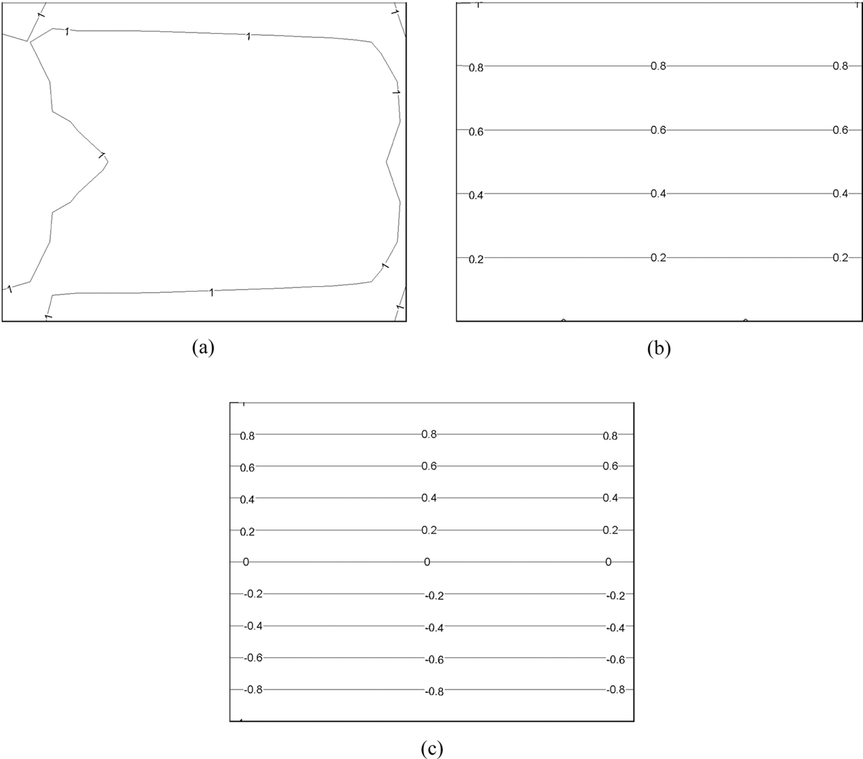
Distribution of normal force Nxx for the cross-ply laminate (0°/90°), for N 0 = 1, simply supported (SS)-I and clamped (C)-I edges. (a) α = 0, (b) α = 1, and (c) α = 2.
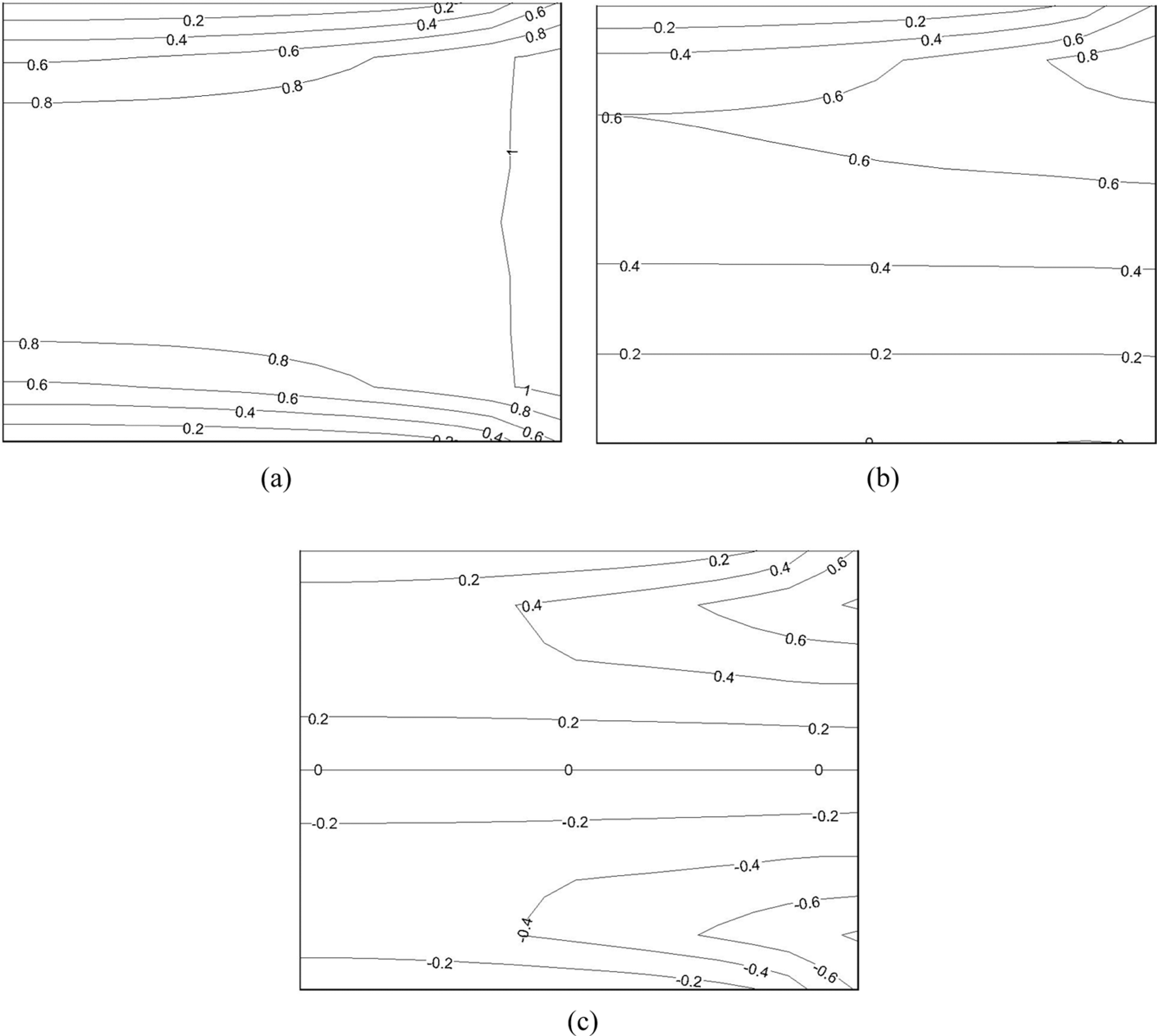
Distribution of normal force Nxx for the cross-ply laminate (0°/90°) s , for N 0 = 1, simply supported (SS)-II and clamped (C)-II edges. (a) α = 0, (b) α = 1, and (c) α = 2.
Design for maximum buckling load
Next, we investigate the effect of various problem parameters on the optimal layer thickness and the maximum buckling load. A four-layered symmetric cross-ply laminate with a stacking sequence (0°/90°/90°/0°) and aspect ratio a/b = 1 is considered. The nondimensional thicknesses of the 0° and 90° plies are given by h 0 = H 0/H and h 90 = H 90/H, respectively, where H 0 and H 90 are the thicknesses of 0° and 90° plies. h 90 can be written in terms of h 0 as h 90 = 0.5 − h 0 so that the unknown is only h 0. Figure 5 shows the curves of λ plotted against h 0 for boundary conditions SS-I and SS-II (Figure 5a) and C-I and C-II (Figure 5b) with α = 0, 1, 2 and b/H = 100. In this figure, λ values are normalized with respect to its value for the equal layer thickness laminate (h 0 = 0.25). It is observed that pure bending, that is, α = 2, yields the highest and the lowest values of λ for all boundary conditions, emphasizing the importance of an optimal design. This case is also more sensitive to the changes in layer thicknesses compared to α = 0 and α = 1. The least sensitiveness to h 0 are due to the cases for α = 0, 1 for the boundary conditions SS-I and C-I. Thus, an optimal design based on these boundary conditions will show little improvement over the laminate with equal thickness layers (h 0 = h 90 = 0.25). It is also observed that the optimal values of h 0, in general, depend on the presence or absence of in-plane boundary restraints. Furthermore, the buckling load of cross-ply laminates can be increased considerably by optimal thickness design if the boundaries are restrained against in-plane movement, that is, for SS-II and C-II. For SS-II and α = 2, the increase in the buckling load is more than 50% as compared to a laminate with equal layer thicknesses (Figure 5a), and the corresponding value for C-II and α = 2 is 30%. However, the sensitivity of buckling load to the optimal thickness needs to be taken into account in a design situation.
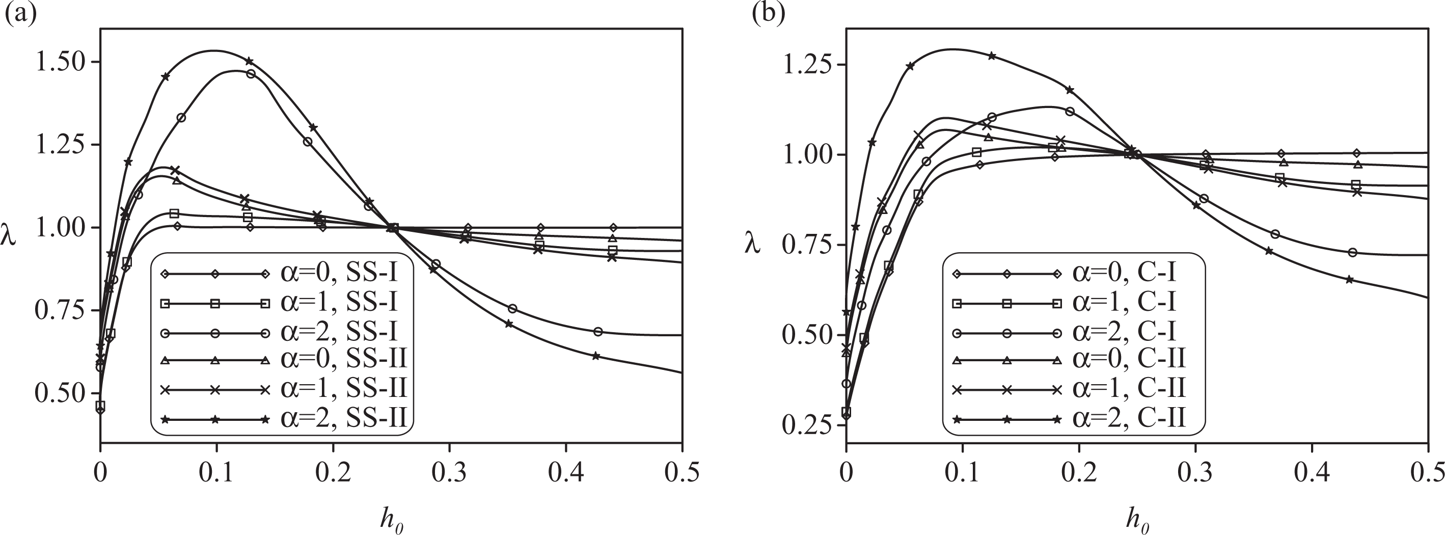
λ versus h 0 for a cross-ply laminate (0°/90°) s , a/b = 0, and b/H = 100.
The corresponding results for b/H = 25 are shown in Figure 6, which shows that the effect of shear deformation on the buckling load is more pronounced in the case of C plates.
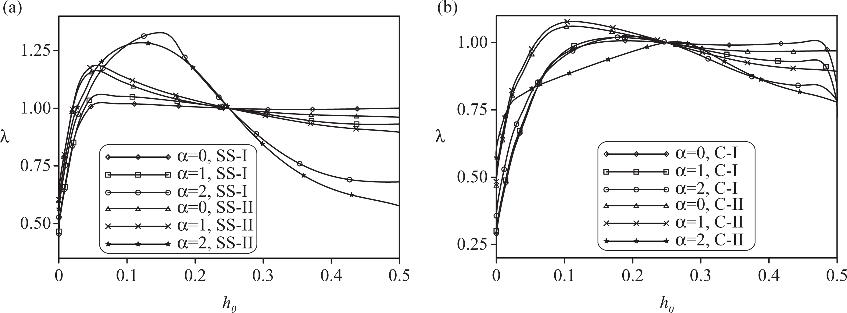
λ versus h 0 for a cross-ply laminate (0°/90°) s , a/b = 1, and b/H = 25.
Optimal layer thicknesses
Numerical results for the design problem stated in Eq. (20) are considered for a (0°/90°/90°/0°) laminate and can be stated as
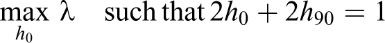
which is a one-dimensional optimization problem which is solved by the Golden section method. The optimization results for the thickness/height ratio b/H = 100 are shown in Tables 4–6 for α = 0, 1, 2, respectively, for different values of the aspect ratios a/b. In these tables, λ0 corresponds to the case h
0 = 0.25, that is equal layer thickness laminate. λmax and h
opt denote the maximum value of the nondimensional buckling load λ and the optimal value of h
0. Efficiency (η) is defined as
Optimization results for α = 0 (uniform edge load), b/H = 100
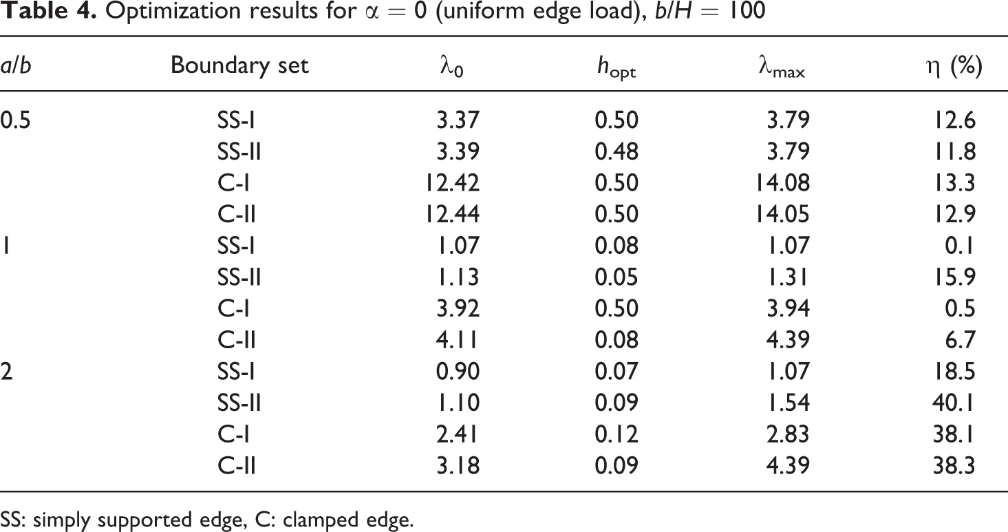
SS: simply supported edge, C: clamped edge.
Optimization results for α = 1 (triangular edge load), b/H = 100
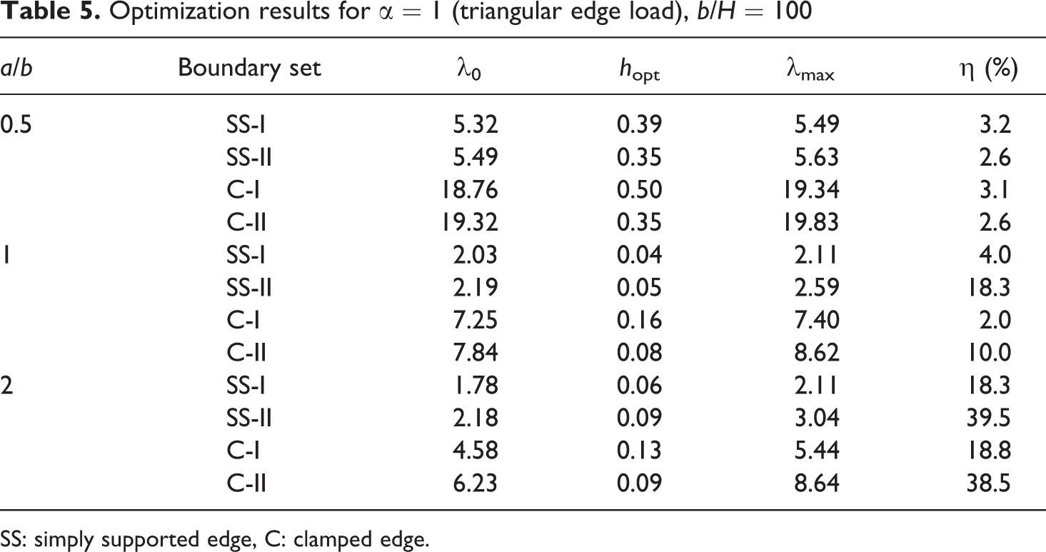
SS: simply supported edge, C: clamped edge.
Optimization results for α = 2 (pure bending edge load), b/H = 100
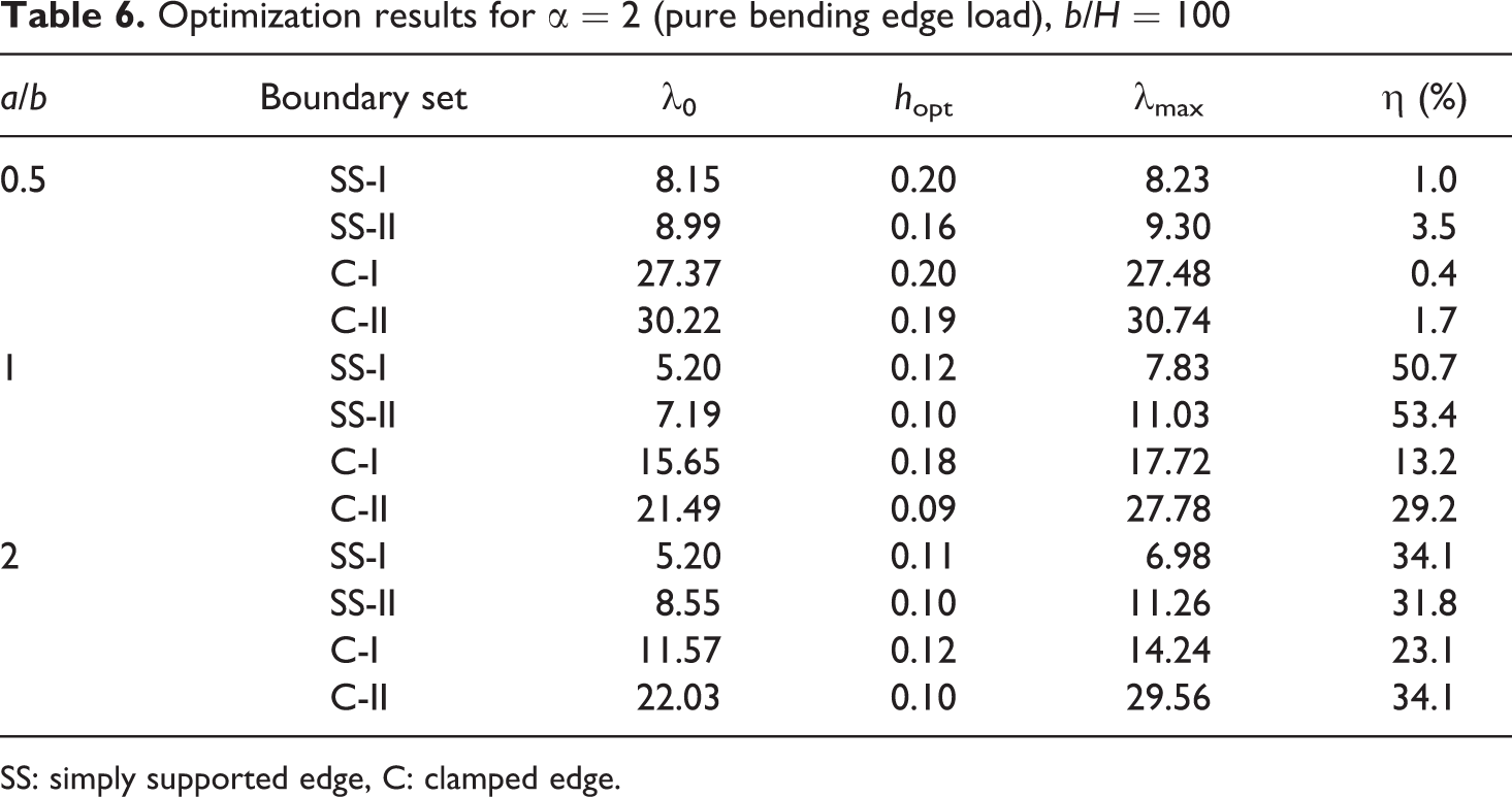
SS: simply supported edge, C: clamped edge.
It is observed that the aspect ratio a/b = 2 and α = 2, in general, gives higher design efficiency; however, the highest efficiencies (more than 50%) are obtained for the aspect ratio a/b = 1 and α = 2 (Table 6). The optimal values of the layer thickness h opt depend on the specific boundary condition and in particular on the absence or presence of boundary restraints as can be seen by comparing the results for SS-I with SS-II and C-I with C-II. Thus, in applications where such restraints exist, neglecting them will lead to suboptimal designs. Comparing the buckling loads of laminates with SS-I and SS-II indicates that restrained boundaries (SS-II) lead to higher buckling loads. Moreover, the difference increases with increasing aspect ratio. Similar results hold for C-I and C-II. It is observed that in the case of pure bending (α = 2; Table 6), h opt remains fairly uniform for a given aspect ratio.
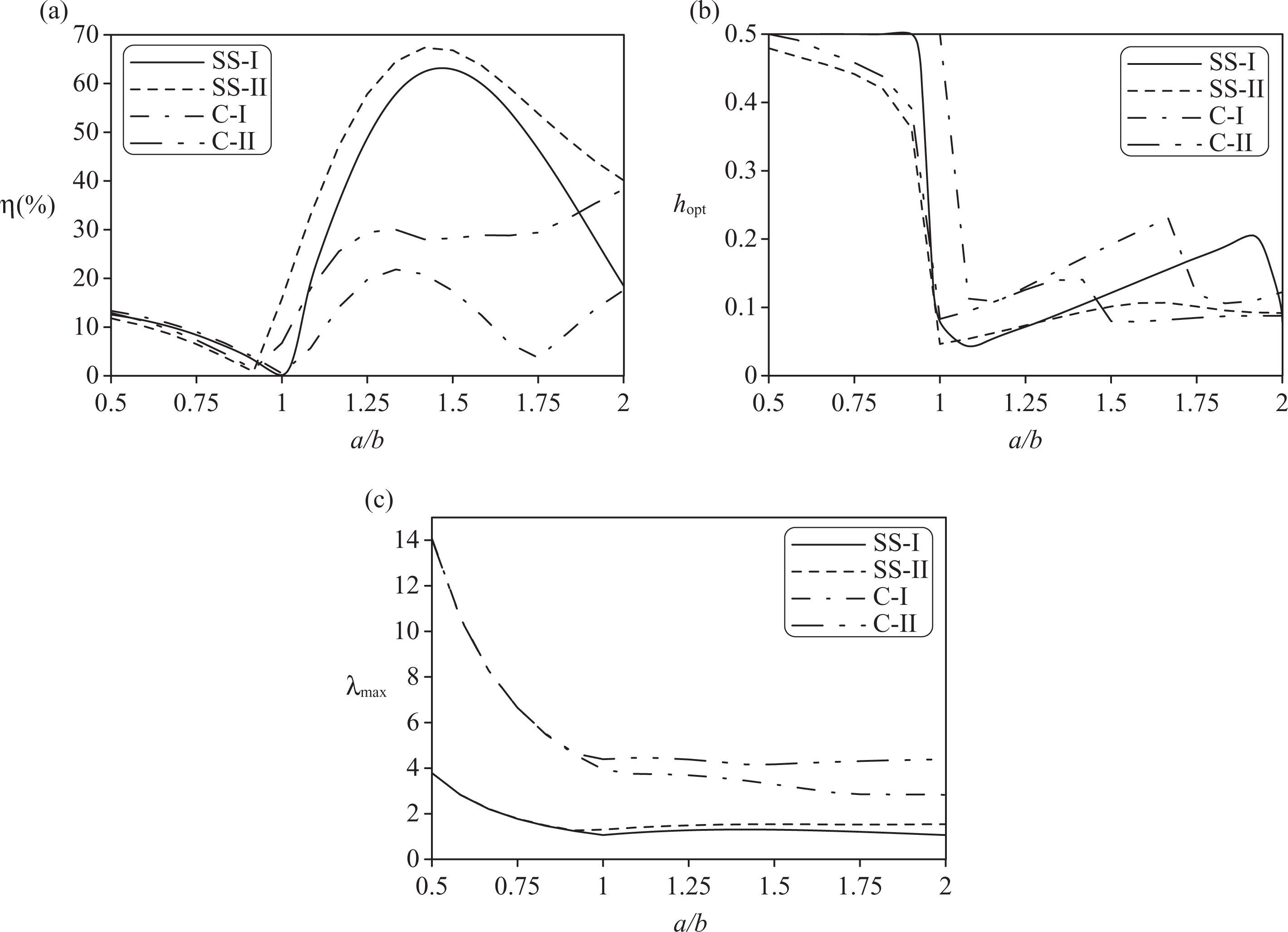
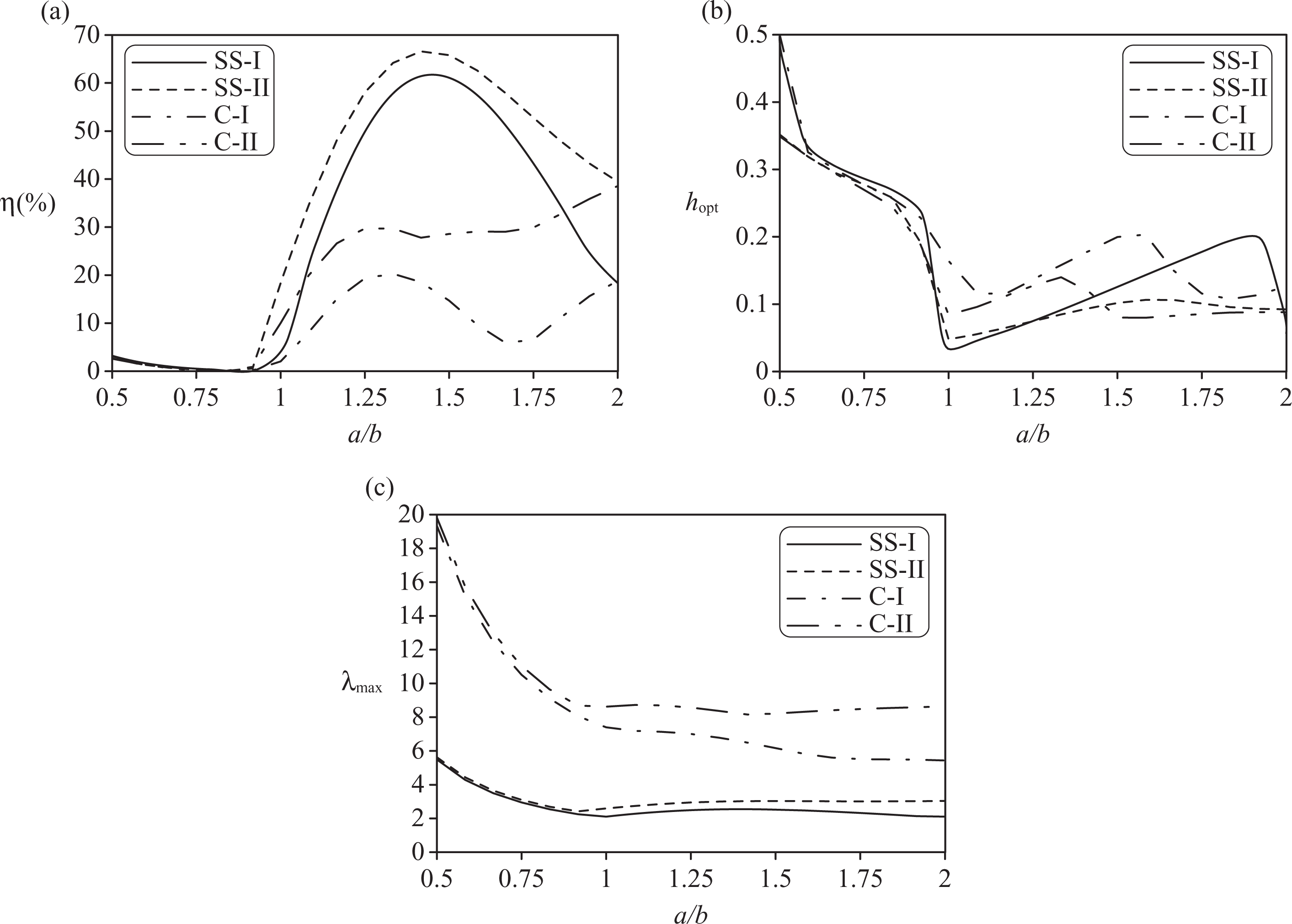
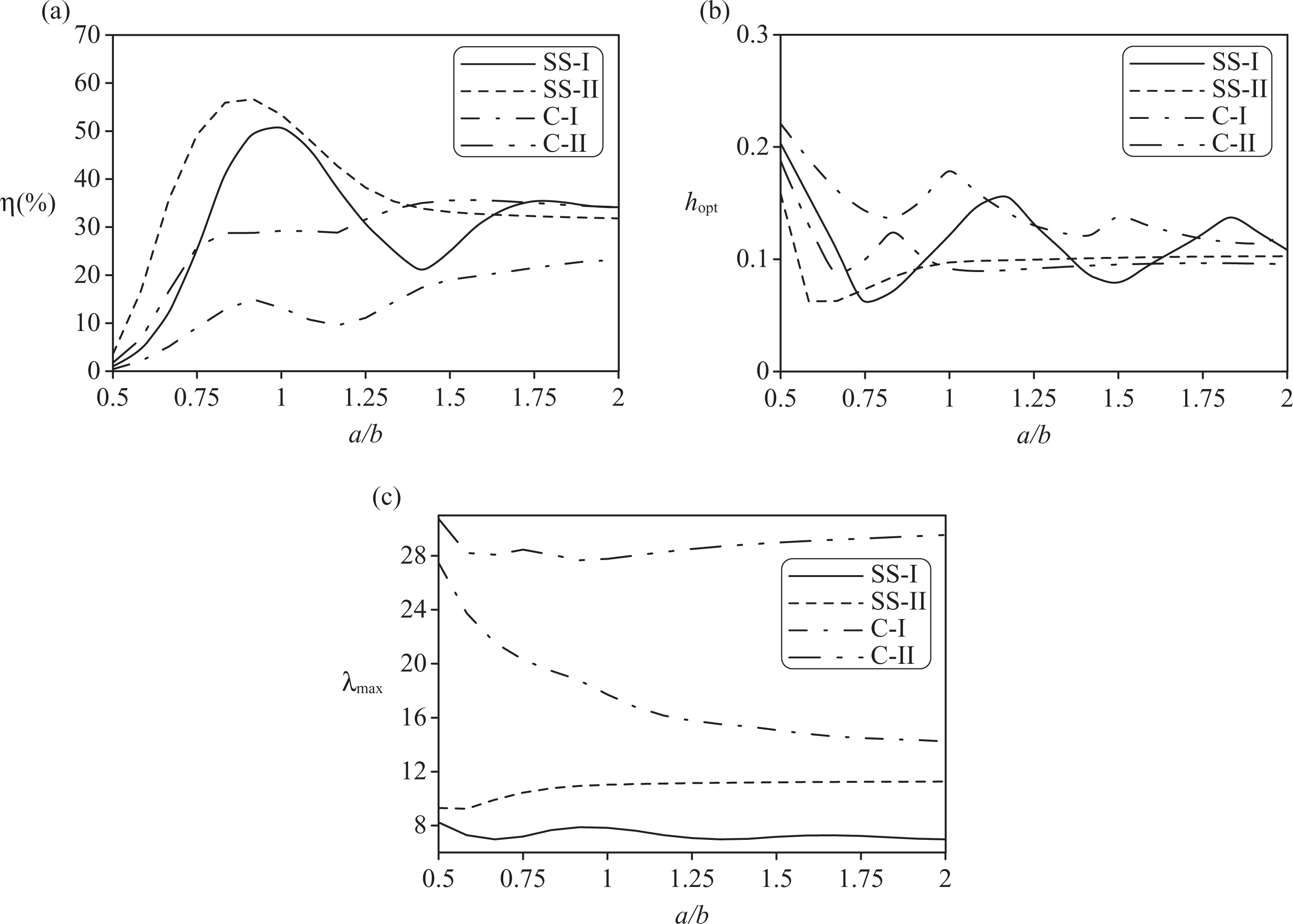
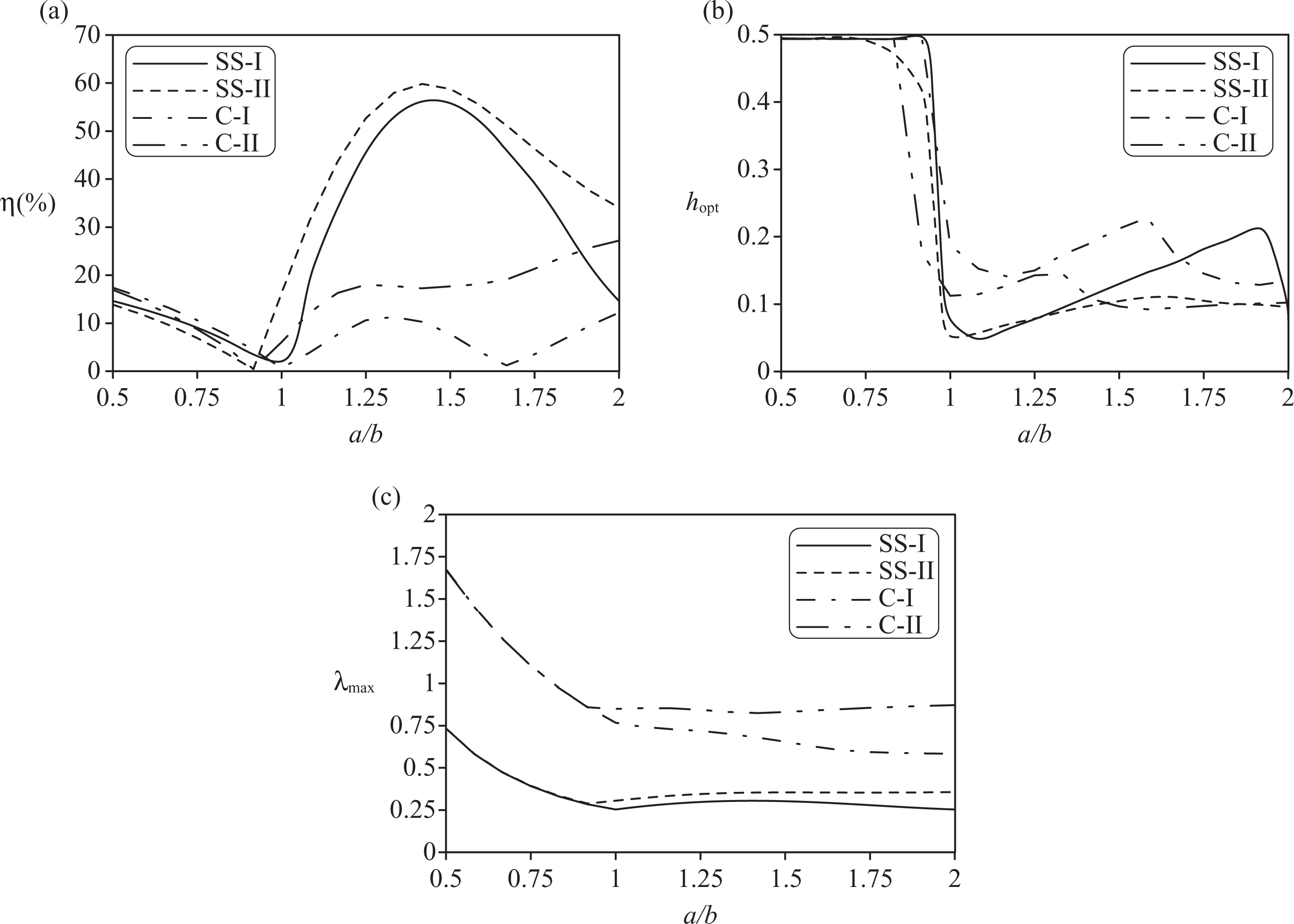
Next the effect of the aspect ratio on the efficiency, optimal layer thickness, and the maximum buckling load is studied. Corresponding results for b/H = 25 are tabulated in Tables 7–9. Results for efficiency, h opt, and λmax versus the aspect ratio are given for α = 0 in Figure 7, for α = 1 in Figure 8, and for α = 2 in Figure 9 for SS-I, SS-II, C-I, and C-II (restrained boundaries) with b/H = 100. It is observed that efficiencies and the optimal h 0 are not monotonic functions of the aspect ratio and h opt fluctuates in a bigger range for α = 0 (Figure 7b) and a smaller range for α = 2 (Figure 9b). Optimization results for b/H = 25 are shown in Figures 10 –12. It is observed that the shear deformation has the largest effect on the optimal layer thicknesses of laminates under pure bending edge loads, that is α = 2 as a comparison of Figures 9 and 12 indicates.
Efficiency, h opt, and buckling load versus a/b, α = 0 (uniform edge load), and b/H = 100.
Efficiency, h opt, and buckling load versus a/b, α = 1 (triangular edge load), and b/H = 100.
Efficiency, h opt, and buckling load versus a/b, α = 2 (pure bending edge load), and b/H = 100.
Efficiency, h opt, and buckling load versus a/b, α = 0 (uniform edge load), and b/H = 25.
Efficiency, h opt, and buckling load versus a/b, α = 1 (triangular edge load), and b/H = 25.
Efficiency, h opt, and buckling load versus a/b, α = 2 (pure bending edge load), and b/H = 25.
Optimization results for α = 0 (uniform edge load), b/H = 25
SS: simply supported edge, C: clamped edge.
Optimization results for α = 1 (triangular edge load), b/H = 25
SS: simply supported edge, C: clamped edge.
Optimization results for α = 2 (pure bending edge load), b/H = 25
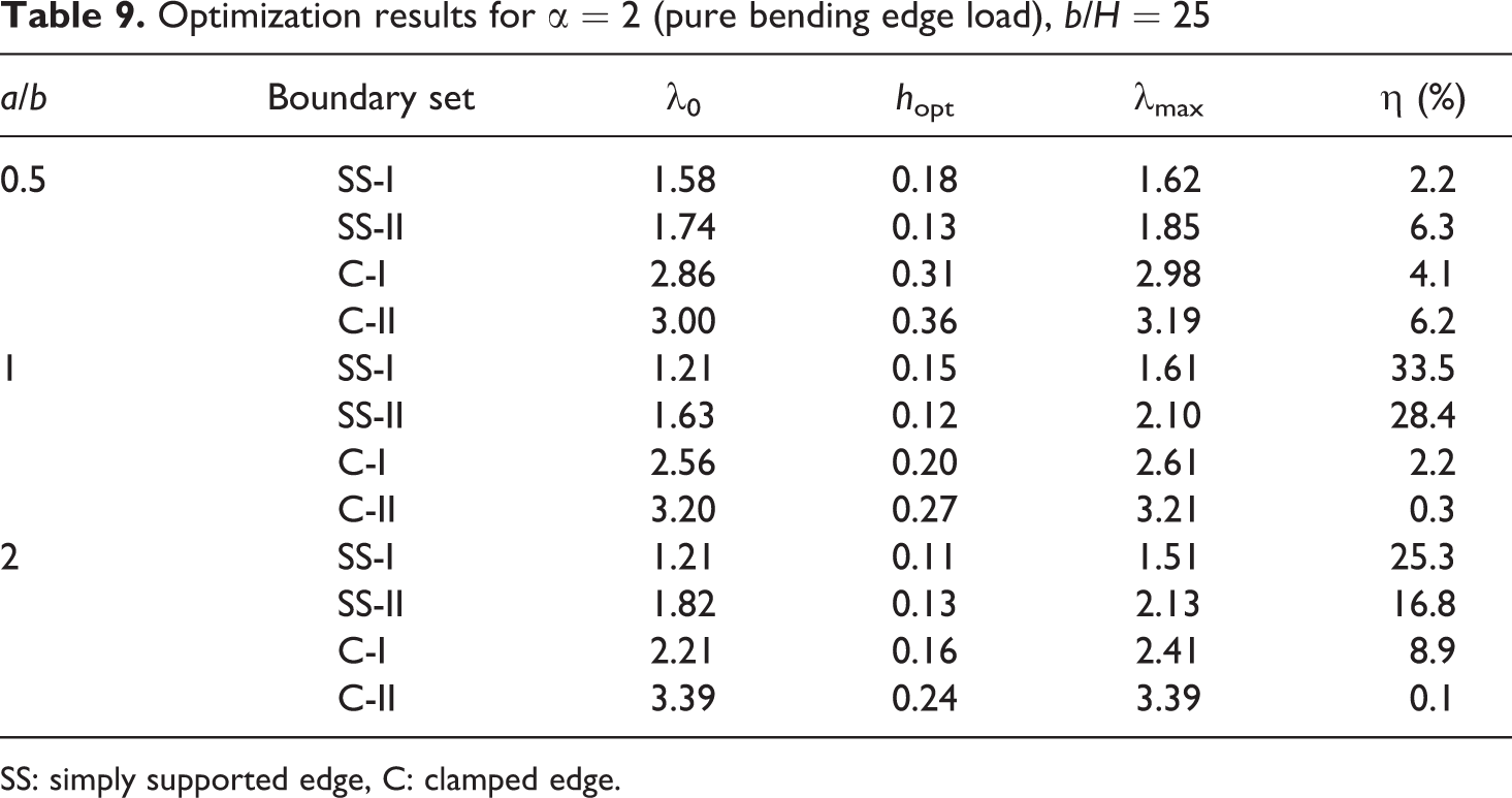
SS: simply supported edge, C: clamped edge.
Conclusions
The effect of in-plane boundary restraints was investigated using the in-plane prebuckling stresses of cross-ply laminates under linearly varying edge loads. Results were given for several combinations of boundary restraints in the form of counter lines. Three edge loads were studied, namely uniform compression for comparison purposes, triangular compressive load, and pure bending edge load. The constant stress distributions under these loads were also shown, which occur under specific boundary conditions that do not apply when the in-plane movement of the plate is constrained. After analyzing the buckling loads with respect to layer thicknesses (Figures 5 and 6), results for the optimal layer thicknesses are given in table and graphical form for various boundary conditions and edge loads. The results presented in the tables were obtained for rectangular plates with aspect ratios a/b = 0.5, 1, 2 under six different combinations of boundary conditions and include the efficiencies of the optimal designs. As there are no analytical solutions for the problems formulated in the present study due to the complicating factors, a finite element method was developed and implemented to calculate the buckling loads and prebuckling stresses. The solution is based on the FSDT and the influence of thickness, that is the contribution of shear deformation was examined by taking the b/H ratio as equal to 25 and 100.
Numerical results show that, as expected, the buckling loads are higher for C plates compared with SS plates, and the presence of in-plane restraints causes an increase in buckling load and, in general, the efficiency increases as a/b and nonuniformity of the edge loads, that is, increase in α.
Footnotes
Acknowledgments
The financial assistance of National Research Foundation of South Africa (NRF) is gratefully acknowledged.
Funding
This research received no specific grant from any funding agency in the public, commercial, or not-for-profit sectors.